Optimal Scheduling of Distributed Energy Resources in Residential Building under the Demand Response Commitment Contract

Abstract

This study proposes optimal day-ahead demand response (DR) participation strategies and distributed energy resource (DER) management in a residential building under an individual DR contract with a grid-system operator. First, this study introduces a DER management system in the residential building for participation to the day-ahead DR market. The distributed photovoltaic generation system (PV) and energy-storage system (ESS) are applied to reduce the electricity demand in the building and sell surplus energy on the grid. Among loads in the building, lighting (LTG) and heating, ventilation, and air conditioning (HVAC) loads are included in the DR program. In addition, it is assumed that a power management system of an electric vehicle (EV) charging station is integrated the DER management system. In order to describe stochastic behavior of EV owners, the uncertainty of EV is formulated based on their arrival and departure scenarios. For measuring the economic efficiency of the proposed model, we compare it with the DER self-consuming operation model without DR participation. The problem is solved using mixed integer linear programming to minimize the operating cost. The results in summer and winter are analyzed to evaluate the proposed algorithm’s validity. From these results, the proposed model can be confirmed as reducing operation cost compared to the reference model through optimal day-ahead DR capacity bidding and implementation.

1. Introduction

Given the current energy and environmental conditions, renewable energy generation facilities capable of fossil fuels are rapidly increasing, and research on distributed energy resources (DERs) in the microgrid are proceeding expeditiously with decarbonization policies. Additionally, utilizing demand response (DR) facilitates customers’ interaction and responsiveness as a producer role, brings short-term advantages to the electricity market, and results in economic benefit for both customers and the grid utility. Furthermore, curtailing demand from a long-term point of view reduces the overall capital cost investment for plant construction and network upgrade and improves the power system reliability [1,2]. In our current society, the efforts described above are applied in the operation of residential building resources since they account for 36% of global energy consumption and 40% of total carbon dioxide emissions, which increase by 2.5% each year [3].

For the above reasons, basic research related to the operation of DERs in residential buildings including renewable energy sources is being advanced. Due to high capacity, easy control, and immediate reaction rate, research on the use of heating, ventilation, and air conditioning (HVAC) load resource of the residential building is concentrated. Stamatescu et al. proposed a smart building with HVAC systems and grid integration [4]. Furthermore, Zhao et al. modeled HVAC control of the residential building that can contribute to the frequency regulation of the grid system [5,6], and Wang et al. studied linear dynamic model for building a HVAC control system using a heuristic algorithm [7]. Additionally, combining lighting (LTG) and HVAC systems with building energy management system is being investigated. The U.S. Department of Energy emphasizes the overall benefits of building resource integration systems that include HVAC and LTG [8]. Motegi et al. discussed lighting control with HVAC of residential buildings as a DR [9]. The residentialization of renewable energy resources has led to diversification in the research on DERs in buildings. Photovoltaic generation (PV), energy storage systems (ESSs), electric vehicle (EV) charging stations, and DR are considered the DER of residential buildings in previous studies [10,11,12,13]. Ren et al. modeled a multi-objective linear programming-based operation algorithm with renewable energy resources according to the electricity rate and fuel gas rate [14]. Research on ESS application in the building DER operation systems has been performed to ensure the stable provision of renewable energy sources [15,16,17,18]. As the spread of EV supply increases, the integration between EV charging stations and the grid system, namely vehicle-to-grid (V2G), has been studied as an additional DER of the building [19]. Sousa et al. modeled the day-ahead DER optimization schedule algorithm with EV charging station constraints [20]. Furthermore, studies on the operation control of electric heating or heat storage systems in the building are intensively carried out to utilize thermal energy as DR resources [21,22,23].

The aforementioned studies involve research on robust DER optimization including DR issuance assumption with unexpected circumstances. Furthermore, there have been studies on optimizing DR participation using DERs. Pipattanasomporn et al. proposed an intelligent home energy management algorithm for managing high-power-consumption household appliances with simulation for DR analysis [24]. Chen et al. evaluated real-time-priced DR management for residential appliances via stochastic optimization [25]. Korkas et al. considered DR management under thermal comfort requirements and created a robust solution based on changing occupancy patterns in microgrids and weather conditions [26]. Gao et al. modeled the robust demand control of residential buildings under load prediction uncertainty [27].

The DR program is well worth exploiting in terms of system operation and is continuously encouraged through political assistance [28,29,30,31]. Nevertheless, due to consistent and generic DR promotion policies, statistical data [32] show that the rate of DR participation by residential building operators still remains low. Besides, according to the aforementioned studies, there has been a paucity of concern about the optimal design of participating capacity under the specified DR contract conditions. To compensate for the deficiency, this study presents a practical optimization algorithm of day-ahead residential building resource operation including DR participation to contribute to the grid system. The proposed model includes:

• Assessment of DR potential considering PV generation,
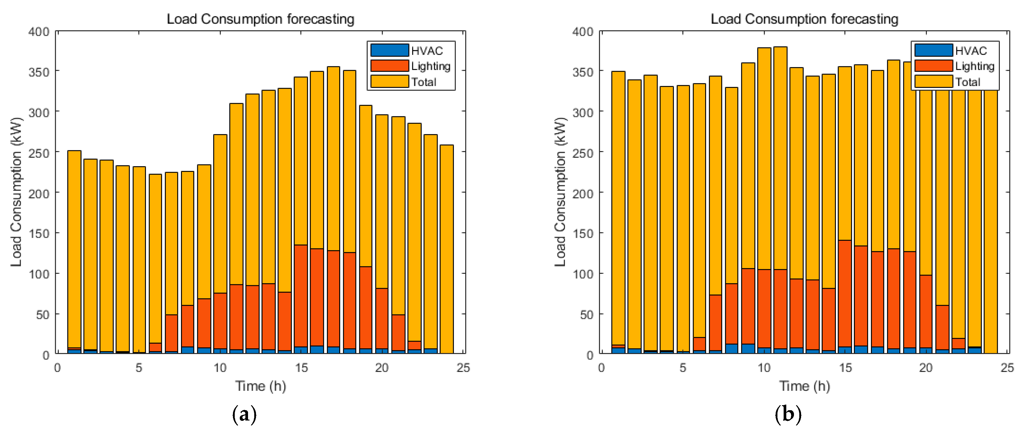
• Load model of LTG and HVAC for DR participation,
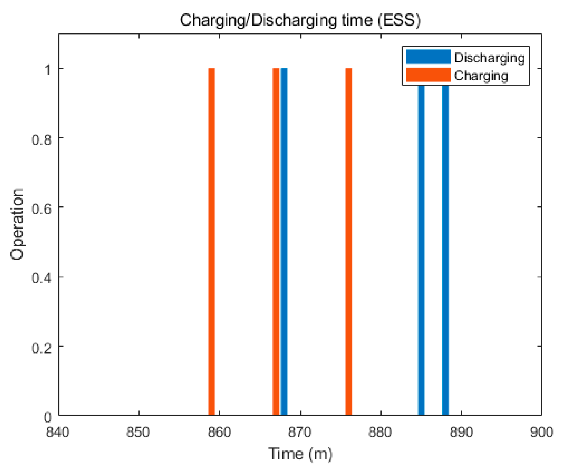
• ESS SOC management including prevention of simultaneous charging/discharging,
• EV SOE management with EV owner’s behavior uncertainty.

The algorithm’s objective involves minimizing operating costs under conditions that reflect contractual DR settlement, and the PV and ESS installation promotional rates [33,34,35,36]. Financial incentives are designed to encourage the spread of renewable energy generation systems by helping to reduce the cost of system installation. Direct cash incentives and tax credits are the two most common types of financial incentives. Direct cash incentives include rebates, subsidies, and performance-based incentives, which reduce the initial cost of operating a renewable energy system and fund investments in loans, power purchase agreements, or property-assessed clean energy (PACE) financing. After the renewable energy generation system is installed, it is possible to obtain financial support continuously in the form of tax benefits [37]. In the US, the introduction of financial incentive policies for renewable energy has achieved grid parity of PV system installations in most states [38]. In Germany, by applying renewable energy policy named Erneuerbare-Energien-Gesetz (EEG), the goal is to achieve a share of renewable energy in gross electricity power production of 35% by 2020 and of 80% by 2050 [39]. In this study, incentives of renewable energy sources are included in the DR contract to encourage the diffusion of renewable energy generation systems. It is assumed that a separate meter is used for monitoring each source, and the amount of DR participation involves net demand reduction of the whole residential building DER system.

In the case of summer and winter, the DER self-consuming operation model and the DER operating model under the DR individual contract conditions are respectively simulated and the results are compared to evaluate how much the proposed model has improved.

The rest of the paper is organized as follows: Section 2 presents the DER operation system in the residential building and subsequently proposes an optimization algorithm of day-ahead scheduling strategy. To generate hourly scenarios, uncertainties associated with the system are defined mathematically. The optimization model is formulated in Section 3, and objective functions and constraints are established precisely. In Section 4, optimization simulation results are enumerated and discussed. Finally, this study’s conclusions are described.

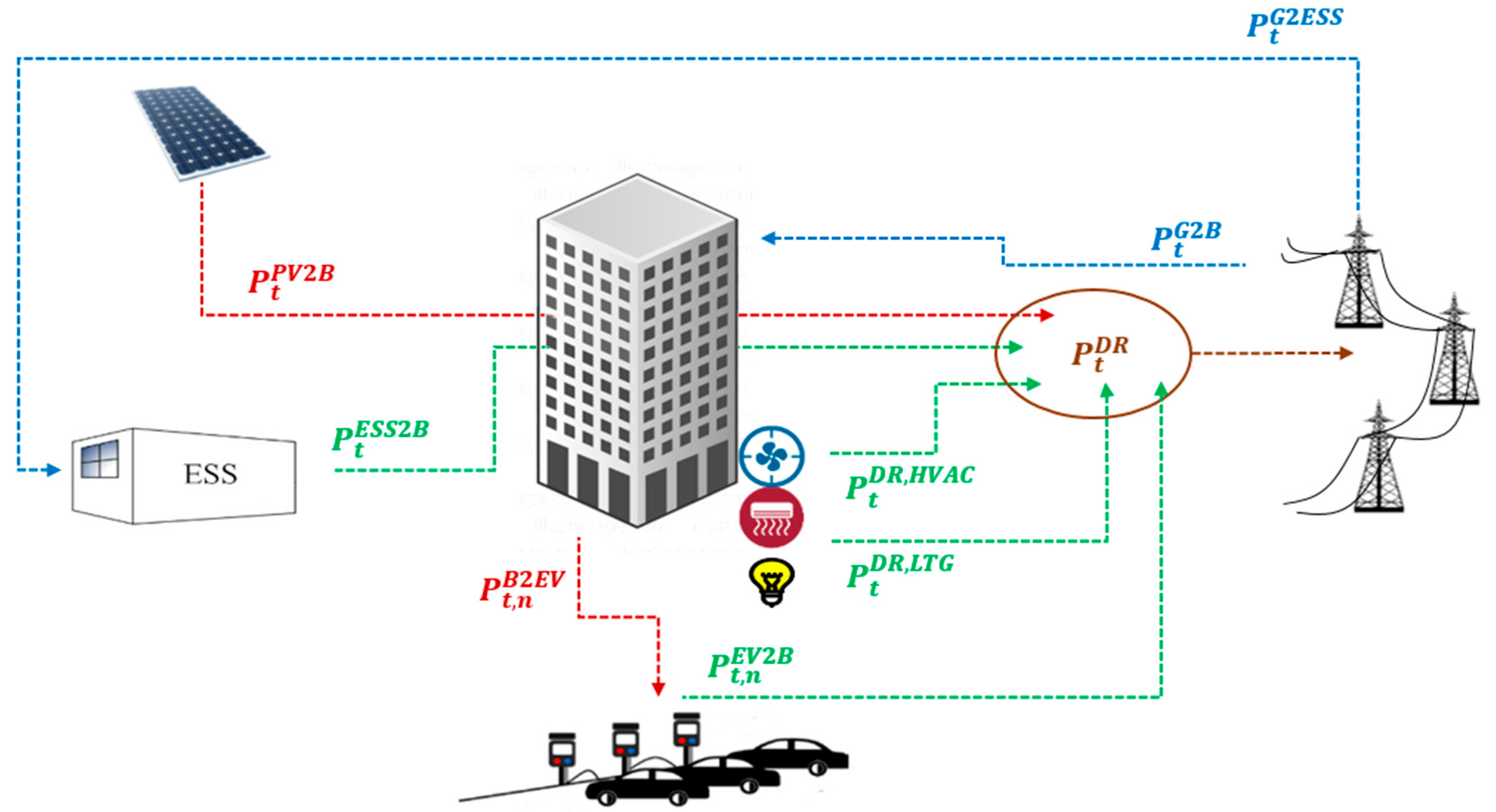
2. DER Operation System in the Residential Building

2.1. Residential Building Energy System Overview

The DER operation system consists of PV, ESS, and EV charging station. All energy produced by the PV is used to reduce the building’s load demand. The ESS helps reduce the building load by charging from the grid during off-peak times and discharging to the building during peak times. The EV charging station is installed in the parking lot of a residential building and exchanges energy with the battery of parked EVs to contribute to the building’s net energy reduction [40,41]. The building system operator is assumed to be able to earn revenues from the operation of the EV charging station through power supply contract with the grid system operator. Depending on the DR contract terms issued in peak time zones, energy resources are determined to have an appropriate DR participation capacity. In addition to the above-described resources, energy resources include LTG and HVAC, which are demand-reduction resources within buildings. The structure of the DER operation system in DR participation time interval is shown in Figure 1.

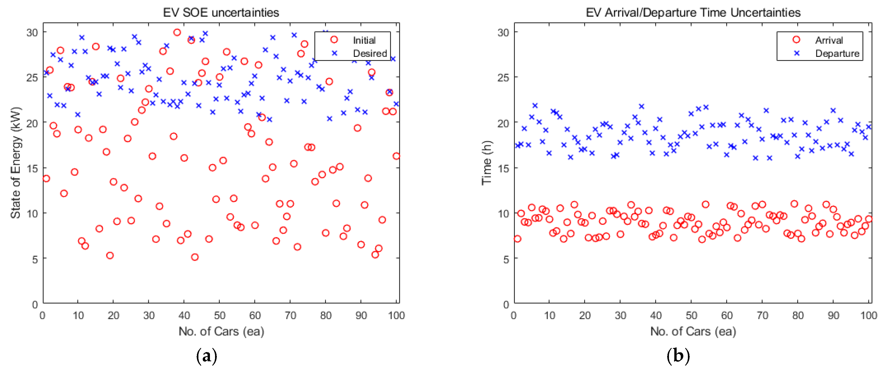
2.2. Uncertainty Modeling of EV

Optimizing scheduling the day before operation requires considering uncertainties in the DER operation model. Therefore, the proposed model has three factors of uncertainty, namely PV generation efficiency, building peak-load consumption, and the status of each EV in the charging station. Proper probability density functions (PDFs) have to be chosen for each DER to reflect the uncertainties and create simulation scenarios [42]. For example, the beta PDF can be used to describe the distribution of irradiance that influences the PV output at a specific location [43]. However, the uncertainties of PV generation and building peak-load consumption are omitted from the formulas in this study because their actual data are used for this study’s experiment. The following scenario creation method is proposed for EV status information.

Status of EVs

Scenarios of EV stats are commonly generated based on truncated Gaussian PDF that can reflect the pattern of EV owners’ behavior, such as arrival time, departure time, and state of energy (SOE) in the probability distribution [44,45,46]. Hence, the formulation is modeled as given in Equations (1a)–(1d).

$$P_n^{SOE,ini}=f_n^{TG}(x;{\mu }^{SOE};{\sigma }^{SOE};(P^{SOE,ini,\min };P^{SOE,ini,\max }))$$

(1a)

$$P_n^{SOE,des}=f_n^{TG}(x;{\mu }^{SOE};{\sigma }^{SOE};(P^{SOE,des,\min };P^{SOE,des,\max }))$$

(1b)

$$t_n^{arv}=f_n^{TG}(x;{\mu }^{arv};{\sigma }^{arv};(t^{arv,\min };t^{arv,\max }))$$

(1c)

$$t_n^{dep}=f_n^{TG}(x;{\mu }^{dep};{\sigma }^{dep};(t^{dep,\min };t^{dep,\max }))$$

(1d)

$f^{TG}$ indicates the truncated Gaussian PDF with a mean of $\mu$ and a variance of ${\sigma }^2$. EV owners want to discharge from their EV batteries to sell the electricity to the market while also charging the batteries to drive. Therefore, as shown in Figure 2, the random initial SOE and desired SOE of EVs are generated within the minimum battery capacity range in which the EV can operate. The arrival and departure time boundaries are set based on the parking duration pattern of the commuting vehicles.

2.3. Structural Framework of the Scheduling Method

Since the decision to participate in DR through the contract is done the day before, it is important to establish a day-ahead time-based operational strategy for each DER based on forecasted generation and consumption. In this study, the optimal day-ahead strategies of DERs and DR capacity are developed considering related uncertainties. The scenarios of PV generation and load consumption of the building are created by importing the forecasted data set. The scenarios of SOE and the time variable for EVs are randomly created using the aforementioned truncated Gaussian PDFs. Subsequently, the optimal scheduling model is constructed with the generated scenarios. The model involves an objective function, namely the net cost minimization of the residential building operation. The model also adopts ESS, EV, LTG, HVAC, and the overall power balance constraints. In addition, the operation plan iterates calculations toward the optimal result based on the reward and penalty price condition. Figure 3 shows the scheduling method’s structural framework.

3. Optimization Model

3.1. Objective Function

In this study, the objective function involves minimizing the operational costs of residential buildings in terms of loss and maximizing revenues from electricity transactions. The loss includes the electricity charge for all the energy used in the building. The revenues contain the benefit of reducing the building load through PV generation, the benefit of operating ESS, the sale of electricity to EVs, and the benefit of DR participation by individual contract with the grid-system operator. The overall objective function is formulated as given in Equations (2a) and (2b) and the following terms of loss and revenues are modeled as shown in Equations (3a)–(3l).

$$Minimize Fn$$

(2a)

$$Fn={\displaystyle \sum _t{L}_t^{elec}-R_t^{PV}-R_t^{ESS}-R_t^{EV}-R_t^{DR}}$$

(2b)

• Term 1: Loss from electricity charges

Term 1 denotes the electricity charge for building load consumption. Electricity costs are divided into the cost for general use and the cost for EV charging and distinguished into contractual basic rate and usage fee; it is formulated in Equation (3a).

$$L_t^{elec}=C^{base,gen}+(P_t^{G2ESS}+P_t^{G2B}-{\displaystyle \sum _n{P}_{t,n}^{B2EV}})\times C_t^{use,gen}+C^{base,EV}+{\displaystyle \sum _n{P}_{t,n}^{B2EV}}\times C_t^{use,EV}$$

(3a)

• Term 2: Revenue from PV generation

Term 2 denotes the revenue from the PV generation. It is expressed as the sum of profits from self-consumption and profits from selling surplus electricity. The profit from self-consumption is a discount on the electricity charge by the amount of PV-generated power used for self-consumption. The profit from selling surplus electricity is calculated by applying the system marginal price (SMP) and renewable energy certificated incentive (REC). The revenue is described as shown in Equations (3b)–(3e).

$$R_t^{PV}=R_t^{PV,self}+R_t^{PV,surp}$$

(3b)

$$R_t^{PV,self}=P_t^{PV,self}\times C_t^{use,gen}\times {\gamma }^{PV,disc}$$

(3c)

$$R_t^{PV,surp}=P_t^{PV,surp}\times (C_t^{SMP}+C^{REC})$$

(3d)

$$P_t^{PV2B}=P_t^{PV,self}+P_t^{PV,surp}$$

(3e)

• Term 3: Revenue from ESS operation

Term 3 denotes the revenue from the ESS operation. It is calculated by adding the basic revenue for encouraging ESS installation and settlement revenue through ESS charging and discharging. The amounts of ESS charging and discharging at peak time zones are used to calculate the basic revenue. The ESS charge amount at the off-peak time zone is applied to estimate the settlement revenue, and the total revenue is formulated as given in Equations (3f)–(3h).

$$R_t^{ESS}=R^{ESS,base}+R_t^{ESS,sett}$$

(3f)

$$R^{ESS,base}={\displaystyle \sum _t(P_t^{ESS2B}-P_t^{G2ESS})}÷P^{reg,gen}\times C^{base,gen}\times {\gamma }^{ESS,inc}, t\in T_{peak}$$

(3g)

$$R_t^{ESS,sett}=P_t^{G2ESS}\times C_t^{use,gen}\times {\gamma }^{ESS,disc}, t\in T_{off-peak}$$

(3h)

• Term 4: Revenue from the sale of electricity to EVs

Term 4 denotes the revenue from the sale of electricity to EVs. The revenue is formulated in Equation (3i).

$$R_t^{EV}={\displaystyle \sum _n(P_n^{SOE,des}-P_n^{SOE,ini}})\times C_t^{EV,ch}$$

(3i)

• Term 5: Revenue from DR participation

Term 5 denotes the revenue from DR participation according to the contract. The DR revenue consists of monthly contractual basic revenue and settlement revenue based on DR participation time interval and capacity. It is formulated as shown in Equations (3j)–(3l).

$$R_t^{DR}=R^{DR,base}+R_t^{DR,sett}$$

(3j)

$$R^{DR,base}=P^{DR,reg}\times C^{DR,base}$$

(3k)

$$R_t^{DR,sett}=P_t^{DR}\times C_t^{SMP}-(P^{DR,reg}-P_t^{DR})\times C_t^{SMP}\times {\gamma }^{DR,pen}$$

(3l)

3.2. Constraints

According to the aforementioned objective function, the constraints involve PV generation, SOC management of ESS, SOE management of EV, DR participation, and power balance. The constraints are defined as follows.

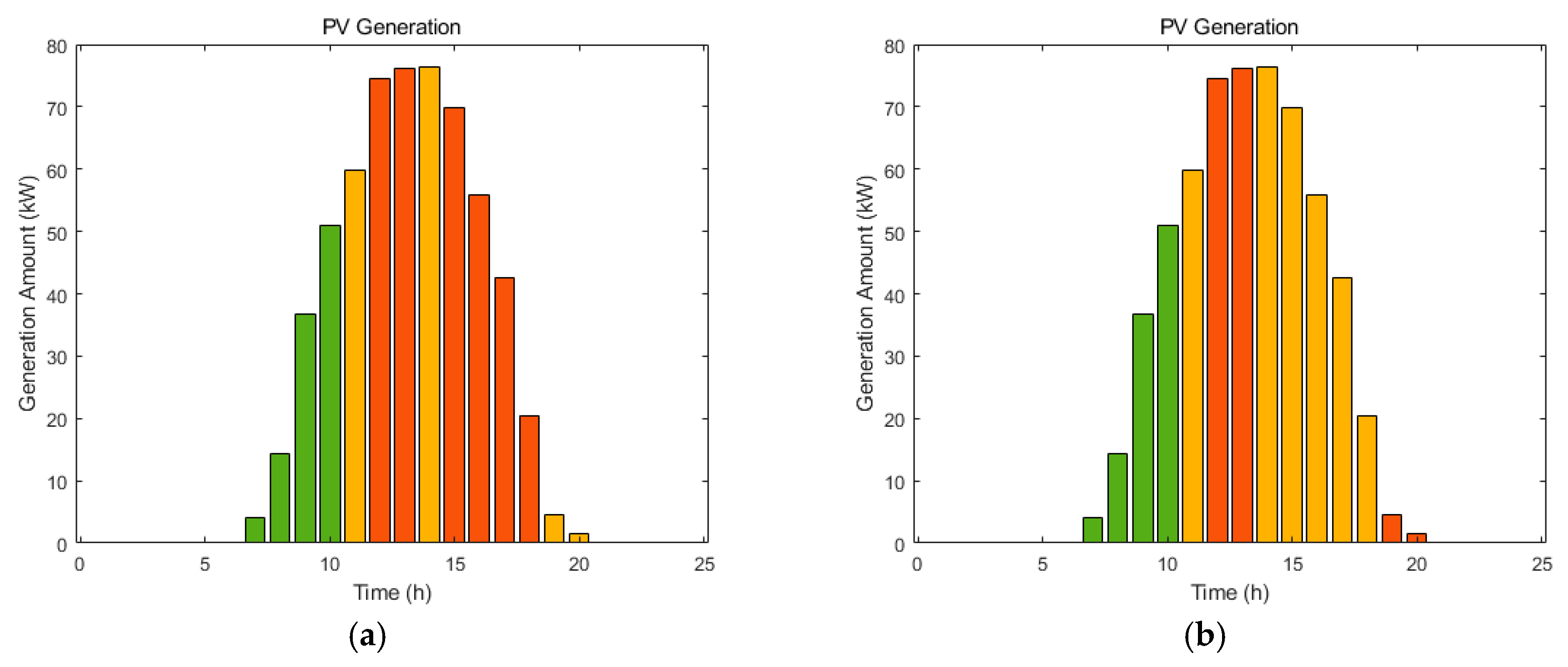
3.2.1. PV Generation

The PV generation amount is scheduled at each time interval within the limitation of the maximum generation capacity as shown in Equation (4).

$$0\le P_t^{PV2B}\le P^{PV2B,\max }$$

(4)

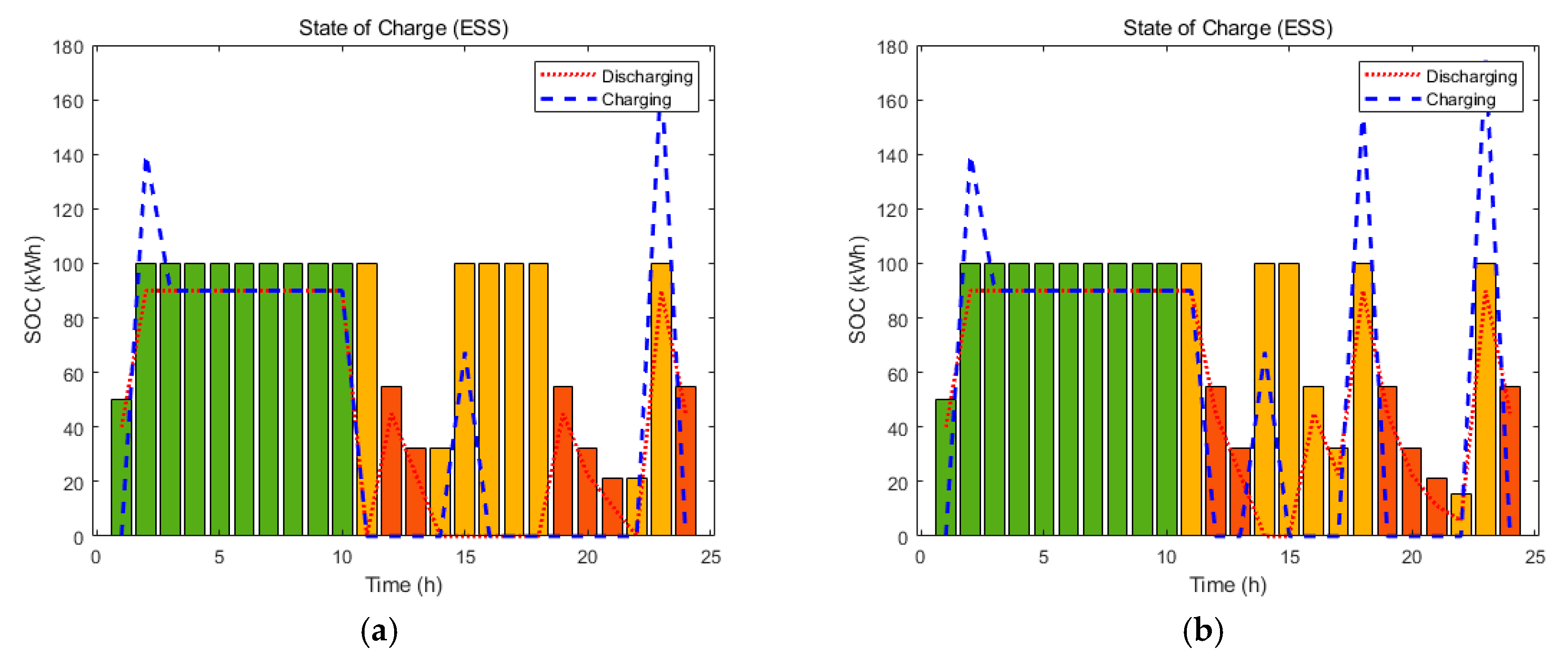
3.2.2. SOC Management of ESS

The charging and discharging speed and efficiency of ESS correspond to constants at every time interval. The unit time interval ($\mathsf{\Delta }t$) is set to an hour and the minimum charging or discharging time interval ($\tau$) is set to a minute. Based on the aforementioned time intervals, the formulation of charging and discharging amount of ESS is as shown in Equations (5a)–(5e).

$$0\le {\tau }_t^{G2ESS}\le \mathsf{\Delta }t$$

(5a)

$$0\le {\tau }_t^{ESS2B}\le \mathsf{\Delta }t$$

(5b)

$$0\le {\tau }_t^{G2ESS}+{\tau }_t^{ESS2B}\le \mathsf{\Delta }t$$

(5c)

$$P_t^{G2ESS}=v^{ESS,ch}\times {\eta }^{ESS,ch}\times {\tau }_t^{G2ESS}$$

(5d)

$$P_t^{ESS2B}=v^{ESS,dch}\times {\eta }^{ESS,dch}\times {\tau }_t^{ESS2B}$$

(5e)

In fact, the simultaneous charging/discharging of the ESS can be prevented by applying the one-minute control variable of the charging/discharging operation. The constraints of the one-minute control of the ESS are omitted since this optimization problem is focused on the hourly schedule of resource operation. Furthermore, once the charge/discharge scheduling time during the time interval is determined, the profit, cost, and SOC at each time interval are unchanged even if the one-minute control is applied. The one-minute control of the ESS is simply implemented with formulating aforementioned constraints in Appendix B.

Based on Equation (5f), the ESS operates within the minimum and maximum limitation of SOC. Equation (5g) is a formulation about the continuity constraint of SOC between each time interval. The initial SOC is arbitrary. The present SOC is derived using the SOC of the previous time interval and the amount of charging and/or discharging at the present time interval.

$$P^{SOC,\min }\le P_t^{SOC}\le P^{SOC,\max }$$

(5f)

$$P_t^{SOC}=P_{t-1}^{SOC}+P_t^{G2ESS}-P_t^{ESS2B}$$

(5g)

The constraints on battery deterioration, depreciation, and performance degradation are omitted to accommodate the conceptual implementation of economically optimal ESS operation scheduling for this study.

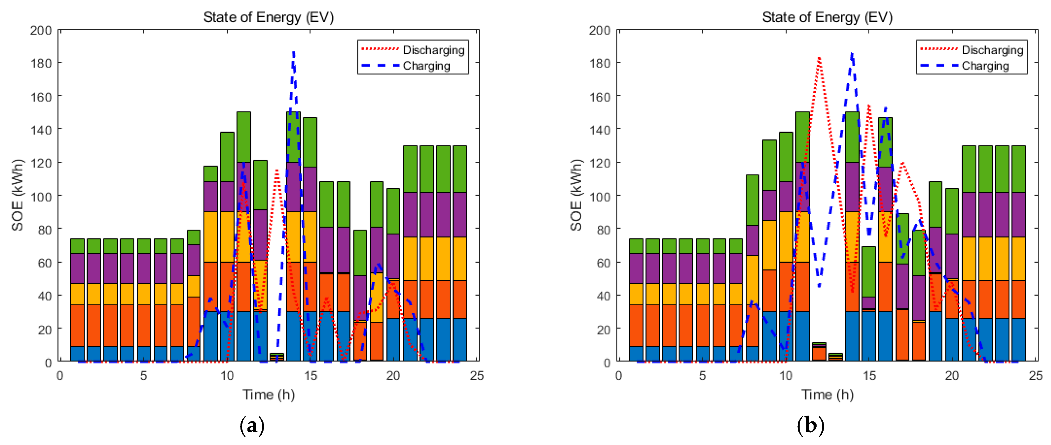
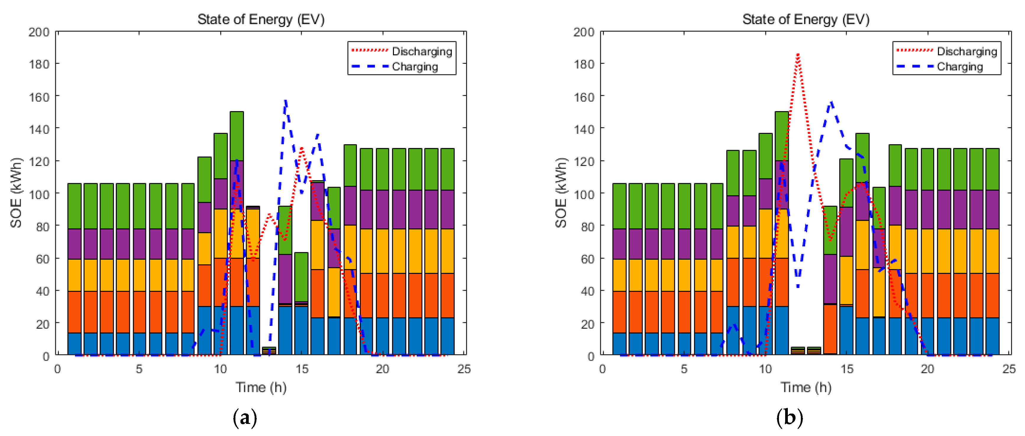
3.2.3. The SOE Management of EV

As shown in Equations (6a)–(6e), (6g) and (6h), the basic contents of the constraints are the same as those of the ESS due to battery characteristics. Additionally, a binary variable is multiplied for the charging equation and the discharging equation to indicate the presence of each EV in the charging station as described in Equations (6c) and (6d). The variable is determined through the generated scenarios of arrival and departure time for EVs. To avoid creating the peak load demand of the building by charging many EV batteries simultaneously, a constraint is additionally complemented as shown in Equation (6f). The EV batteries operate within the minimum and maximum limitation of SOE as described in Equation (6g) and the continuity constraint of SOE between each time interval is formulated as shown in Equation (6h).

$$0\le {\tau }_{t,n}^{B2EV}\le \mathsf{\Delta }t$$

(6a)

$$0\le {\tau }_{t,n}^{EV2B}\le \mathsf{\Delta }t$$

(6b)

$$0\le {\tau }_{t,n}^{B2EV}+{\tau }_{t,n}^{EV2B}\le \mathsf{\Delta }t$$

(6c)

$$P_{t,n}^{B2EV}=v^{EV,ch}\times {\eta }^{EV,ch}\times {\tau }_{t,n}^{B2EV}\times X_{t,n}^{EVinSt}$$

(6d)

$$P_{t,n}^{EV2B}=v^{EV,dch}\times {\eta }^{EV,dch}\times {\tau }_{t,n}^{EV2B}\times X_{t,n}^{EVinSt}$$

(6e)

$${\displaystyle \sum _n{P}_{t,n}^{B2EV}÷\mathsf{\Delta }t}\le P_t^{B2EV,\max }$$

(6f)

$$P^{SOE,\min }\le P_{t,n}^{SOE}\le P^{SOE,\max }$$

(6g)

$$P_{t,n}^{SOE}=P_{t-1,n}^{SOE}+P_{t,n}^{B2EV}-P_{t,n}^{EV2B}$$

(6h)

As expressed in Equations (6i) and (6j), the initial SOE should be the same as that of the arrival time and the desired SOE for EV owners should be equal to that of the departure time.

$$P_{t_n^{arv},n}^{SOE}=P_n^{SOE,ini}$$

(6i)

$$P_{t_n^{dep},n}^{SOE}=P_n^{SOE,des}$$

(6j)

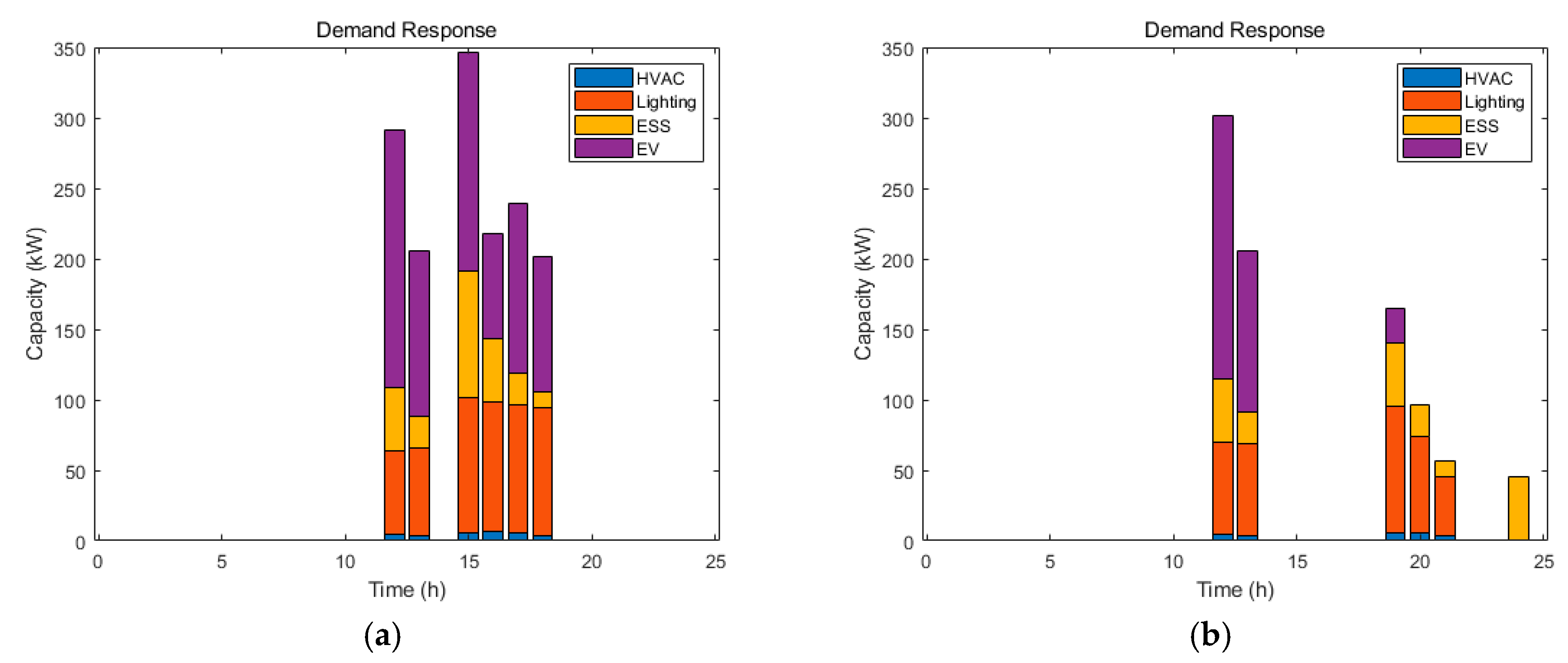
3.2.4. DR Participation

A DR participation plan is considered to reduce the peak load of the grid system at the peak time zone. Typically, HVAC and LTG loads are involved in DR since they can react instantaneously among the load resources of a residential building. In the case of a HVAC load, the average DR participation capacity can be derived in the form of kW per volume for the building’s space [47]. In the case of an LTG load, an illuminance reduction greater than 15% of the initial illuminance can be accepted without inconvenience [48]. Accordingly, the maximum allowable capacity of HVAC and LTG load is determined as shown in Equations (7a) and (7b).

$$P_t^{DR,HVAC,\max }=P_t^{HVAC}\times {\eta }^{DR,HVAC}$$

(7a)

$$P_t^{DR,LTG,\max }=P_t^{LTG}\times {\eta }^{DR,LTG}$$

(7b)

To decide whether to participate in DR, a binary variable is included as in Equations (7c) and (7d).

$$X_t^{DR}\times P_t^{DR,HVAC}\le P_t^{DR,HVAC,\max }$$

(7c)

$$X_t^{DR}\times P_t^{DR,LTG}\le P_t^{DR,LTG,\max }$$

(7d)

As described in Equations (7e) and (7f), the total DR participation capacity at a peak time zone is aggregated and applied in the revenue calculation.

$$P_t^{DR}=X_t^{DR}\times (P_t^{PV,self}+P_t^{ESS2B}+{\displaystyle \sum _n{P}_{t,n}^{EV2B}}+P_t^{DR,HVAC}+P_t^{DR,LTG}), t\in T_{peak}$$

(7e)

$$P_t^{DR}=0, t\notin T_{peak}$$

(7f)

3.2.5. Load Balance

The total amount of electricity consumed by the building precisely corresponds to the amount of electricity provided from the building as shown in Equation (8a). Furthermore, the constraint to limit the electricity usage of the building for each time interval is included for the stable power supply of the grid system as given in Equation (8b).

$$P_t^{G2B}+P_t^{PV2B}+P_t^{ESS2B}+{\displaystyle \sum _n{P}_{t,n}^{EV2B}}+P_t^{DR,HVAC}+P_t^{DR,LTG}=P_t^{LOAD}+{\displaystyle \sum _n{P}_{t,n}^{B2EV}}$$

(8a)

$$P_t^{G2B}\le P^{G2B,\max }$$

(8b)

4. Numerical Studies

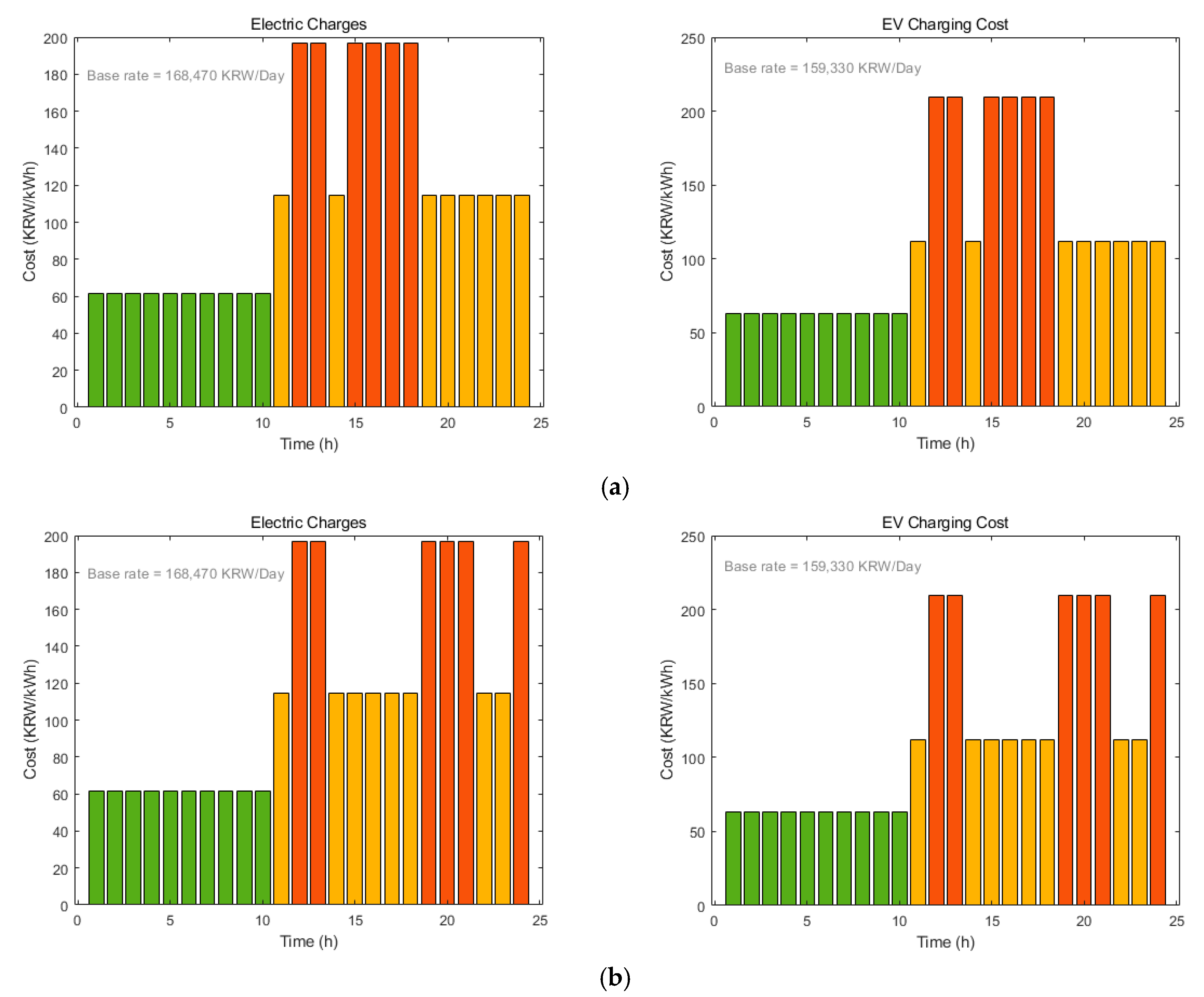
4.1. Case Studies

The proposed model is evaluated by collecting hourly load consumption data of 14 August 2017 for the summer case and 25 January 2017 for the winter case from the building of Research Institute for Solar and Sustainable Energies (RISE) in the Gwangju Institute of Science and Technology (GIST) in Korea.

Table 1. Electricity charge data.

${\mathit{C}}^{\mathit{b}\mathit{a}\mathit{s}\mathit{e},\mathit{g}\mathit{e}\mathit{n}} (\mathbf{KRW}/\mathbf{kWh})$	${\mathit{C}}^{\mathit{b}\mathit{a}\mathit{s}\mathit{e},\mathit{E}\mathit{V}} (\mathbf{KRW}/\mathbf{kWh})$	${\mathit{C}}^{\mathit{R}\mathit{E}\mathit{C}} (\mathbf{KRW}/\mathbf{kWh})$	${\mathit{P}}^{\mathit{r}\mathit{e}\mathit{g},\mathit{g}\mathit{e}\mathit{n}} \left(\mathbf{kW}\right)$	${\mathit{P}}^{\mathit{r}\mathit{e}\mathit{g},\mathit{E}\mathit{V}} \left(\mathbf{kW}\right)$
7220	2390	80	700	200

lists the characteristics of electricity charge. Information data of time-based electricity charge for general usage, EV charging cost, and the SMP are described as shown in Figure 4 and Figure 5. The green bars indicate the off-peak time zone, the yellow bars indicate the mid-peak time zone, and the orange bars indicate the peak time zone.

Further case data of PV generation, ESS characteristics, EV characteristics, DR characteristics, and the load data for the HVAC and LTG in a residential building are described in Appendix A.

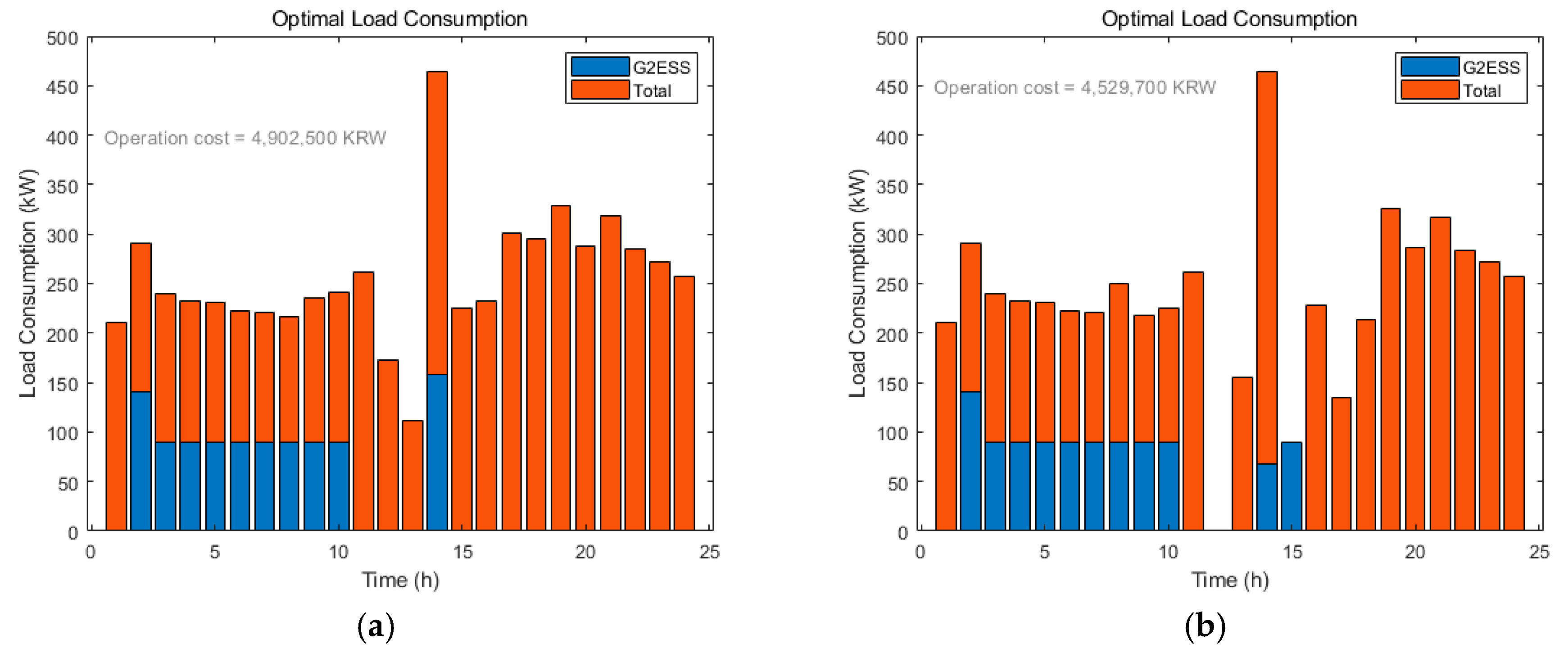
4.2. Simulation Results

To verify the usefulness of DR participation in DER optimal operation, the simulation results of the DER operational optimization excluding DR participation and the DER operational optimization including DR participation are compared for summer and winter. The results are as described as shown in

Table 2. Optimal operation cost comparison.

	Operation Cost without DR (KRW)	Operation Cost with DR (KRW)	Cost Decrease (%)
Summer	4,902,500	4,529,700	7.6
Winter	5,035,700	4,768,100	5.3

.

Previous studies have shown that the generation of peak loads closely correlates with temperature [49,50]. Actually, the load used for heating and cooling occupies a large portion of the total load usage. Therefore, in summer, the peak time zone is biased in the daytime. Figure 6 shows the optimal load consumption scheduling results in the summer case. In the case with DR participation, the overall strategy is to reduce the load during the peak time zones to pursue profits through DR participation.

Figure 7 shows hourly total charge and discharge amount according to charging and discharging scheduling within a unit time. The charging and discharging strategies of the ESS are both the same to gain revenue through charge rate discounts in off-peak time zones. However, in peak time zones, particularly between 15 h and 18 h, there is a big difference in the charging scheduling to consider the DR participation amount after 16 h.

The optimal SOE scheduling results of EVs are the same as those of the ESS because of the battery’s general characteristics. In this experiment, random data of five EVs are applied and the results are color-coded as shown in Figure 8.

In winter, based on the historical load consumption data, peak time zones are divided into daytime and evening after work. Figure 9 shows the optimal load consumption scheduling results in winter. Similar to summer, there is a difference in the load reduction for DR participation between each result.

Based on the simulation results of Figure 10 and Figure 11, it is confirmed that ESS and EVs are involved in load reduction through economical charging and discharging schedules by time zone. The DR participatory model takes a strategy of charging in an off-peak time zone or mid-peak time zone and discharging during peak time zone aggressively to contribute to DR as expected.

The purpose of this study is to validate through experiments that ESS, EV, HVAC load, and LTG load establish the day-ahead optimal operation plan by determining the amount of DR participation as shown in Figure 12. The result has the numerical effect of significantly reducing operating costs compared to the basic DER operation model without DR participation.

4.3. Discussions

The optimization problem of this study is aimed at reducing the operating cost of the building through DR participation scheduling, which can obtain the highest profit, and the experimental results confirm the objective adherence of the algorithm. The optimal scheduling based on the seasonal electricity cost was derived and the load usage avoidance in the peak time zone was achieved only through economic constraints. Operating costs based on actual data were compared between DR participation case and DR non-participation case. As a result, resource management including DR incentive could achieve cost savings of 5–7%. Considering the deterioration cost of ESS and EV and the time-based control of HVAC and lighting loads, more empirical results can be derived.

5. Conclusions

This study proposes an optimal DER management model of a residential building to estimate the day-ahead DR participation capacity and corresponding hourly operation plan of resources. The model was consistent with the DR engagement strategy in a DR contract environment; it was composed of a PV, ESS, EV charging station, HVAC, and LTG load resource for DR. Uncertainties from the DER were defined and applied to generate hourly scenarios and the optimization model was an object to minimize the operation cost of DERs in a residential building. To derive the practical net cost of DER operation, the cost functions of each DER were defined in detail based on electrical energy policies. There were constraints of PV generation, SOC management of ESS, SOE management of EV, DR participation capacity, and load balance in the DER operation optimization model. Case studies of the proposed model were performed by comparing the DER optimization algorithm excluding DR participation and the algorithm including DR participation in both summer and winter cases. The numerical study results verified that the day-ahead optimal operation plan could determine the DR participation capacity and corresponding DER management efficiently by time zone. The model was finally validated by confirming that the operation cost is reduced compared to the reference model.

References

1. Lawrence Berkeley National Lab. Coordination of Energy Efficiency and Demand Response. Available online: https://www.osti.gov/biblio/981732 (accessed on 10 January 2019).
2. Mohagheghi, S.; Stoupis, J.; Wang, Z.; Li, Z.; Kazemzadeh, H. Demand response architecture: Integration into the distribution management system. 2010 First IEEE Int. Conf. Smart Grid Commun. 2010, 501–506. [Google Scholar] [CrossRef]
3. OECD/IEA. Energy Technology Perspectives 2017: Catalysing Energy Technology Transformations. Available online: https://www.iea.org/etp2017 (accessed on 10 January 2019).
4. Stamatescu, G.; Stamatescu, I.; Arghira, N.; Calofir, V.; Fagarasan, I. Building cyber-physical energy systems. Available online: https://arxiv.org/abs/1605.06903 (accessed on 10 January 2019).
5. Zhao, P.; Henze, G.P.; Brandemuehl, M.J.; Cushing, V.J.; Plamp, S. Dynamic frequency regulation resources of residential buildings through combined building system resources using a supervisory control methodology. Energy Build. 2015, 86, 137–150. [Google Scholar] [CrossRef]
6. Zhao, P.; Henze, G.P.; Plamp, S.; Cushing, V.J. Evaluation of residential building HVAC systems as frequency regulation providers. Energy Build. 2013, 67, 225–235. [Google Scholar] [CrossRef]
7. Wang, S.; Xu, X. Parameter estimation of internal thermal mass of building dynamic models using genetic algorithm. Energy Convers. Manag. 2006, 47, 1927–1941. [Google Scholar] [CrossRef]
8. U.S. Department of Energy. Building-to-grid technical opportunities: Introduction and vision. Available online: https://www.energy.gov/eere/buildings/downloads/buildings-grid-technical-opportunities-introduction-and-vision (accessed on 10 January 2019).
9. Lawrence Berkeley National Lab. Introduction to Residential Building Control Strategies and Techniques for Demand Response. Available online: https://www.osti.gov/search/title:Introduction%20to%20residential%20building%20control%20strategies%20and%20techniques%20for%20demand%20response (accessed on 10 January 2019).
10. Connolly, D.; Lund, H.; Mathiesen, B.V.; Leahy, M. A review of computer tools for analysing the integration of renewable energy into various energy systems. Appl. Energy 2010, 87, 1059–1082. [Google Scholar] [CrossRef]
11. Morais, H.; Kádár, P.; Faria, P.; Vale, Z.A.; Khodr, H. Optimal scheduling of a renewable micro-grid in an isolated load area using mixed-integer linear programming. Renew. Energy 2010, 35, 151–156. [Google Scholar] [CrossRef] [Green Version]
12. Vale, Z.; Morais, H.; Khodr, H.; Canizes, B.; Soares, J. Technical and economic resources management in smart grids using heuristic optimization methods. IEEE PES Gen. Meet. 2010, 1–7. [Google Scholar] [CrossRef]
13. Varkani, A.K.; Daraeepour, A.; Monsef, H. A new self-scheduling strategy for integrated operation of wind and pumped-storage power plants in power markets. Appl. Energy 2011, 88, 5002–5012. [Google Scholar] [CrossRef]
14. Ren, H.; Zhou, W.; Nakagami, K.; Gao, W.; Wu, Q. Multi-objective optimization for the operation of distributed energy systems considering economic and environmental aspects. Appl. Energy 2010, 87, 3642–3651. [Google Scholar] [CrossRef]
15. Beaudin, M.; Zareipour, H.; Schellenberglabe, A.; Rosehart, W. Energy storage for mitigating the variability of renewable electricity sources: An updated review. Energy Sustain. Dev. 2010, 14, 302–314. [Google Scholar] [CrossRef]
16. Boicea, V.A. Energy storage technologies: The past and the present. Proc. IEEE 2014, 102, 1777–1794. [Google Scholar] [CrossRef]
17. Pearre, N.S.; Swan, L.G. Technoeconomic feasibility of grid storage: mapping electrical services and energy storage technologies. Appl. Energy 2015, 137, 501–510. [Google Scholar] [CrossRef]
18. Toledo, O.M.; Oliveira Filho, D.; Diniz, A.S.A.C. Distributed photovoltaic generation and energy storage systems: A review. Renew. Sustain. Energy Rev. 2010, 14, 506–511. [Google Scholar] [CrossRef]
19. Yang, Z.; Li, K.; Foley, A. Computational scheduling methods for integrating plug-in electric vehicles with power systems: A review. Renew. Sustain. Energy Rev. 2015, 51, 396–416. [Google Scholar] [CrossRef]
20. Sousa, T.; Morais, H.; Soares, J.; Vale, Z. Day-ahead resource scheduling in smart grids considering vehicle-to-grid and network constraints. Appl. Energy 2012, 96, 183–193. [Google Scholar] [CrossRef]
21. Arteconi, A.; Patteeuw, D.; Bruninx, K.; Delarue, E.; D’haeseleer, W.; Helsen, L. Active demand response with electric heating systems: Impact of market penetration. Appl. Energy 2016, 177, 636–648. [Google Scholar] [CrossRef]
22. Alimohammadisagvand, B.; Jokisalo, J.; Siren, K. Comparison of four rule-based demand response control algorithms in an electrically and heat pump-heated residential building. Appl. Energy 2018, 209, 167–179. [Google Scholar] [CrossRef] [Green Version]
23. Patteeuw, D.; Bruninx, K.; Arteconi, A.; Delarue, E.; D’haeseleer, W.; Helsen, L. Integrated modeling of active demand response with electric heating systems coupled to thermal energy storage systems. Appl. Energy 2018, 151, 306–319. [Google Scholar] [CrossRef]
24. Pipattanasomporn, M.; Kuzlu, M.; Rahman, S. An algorithm for intelligent home energy management and demand response analysis. IEEE Trans. Smart Grid 2012, 3, 2166–2173. [Google Scholar] [CrossRef]
25. Chen, Z.; Wu, L.; Fu, Y. Real-time price-based demand response management for residential appliances via stochastic optimization and robust optimization. IEEE Trans. Smart Grid 2012, 3, 1822–1831. [Google Scholar] [CrossRef]
26. Korkas, C.D.; Baldi, S.; Michailidis, I.; Kosmatopoulos, E.B. Occupancy-based demand response and thermal comfort optimization in microgrids with renewable energy sources and energy storage. Appl. Energy 2016, 163, 93–104. [Google Scholar] [CrossRef]
27. Gao, D.C.; Sun, Y.; Lu, Y. A robust demand response control of residential buildings for smart grid under load prediction uncertainty. Energy 2015, 93, 275–283. [Google Scholar] [CrossRef]
28. Paterakis, N.G.; Erdinç, O.; Catalão, J.P. An overview of Demand Response: Key-elements and international experience. Renew. Sustain. Energy Rev. 2017, 69, 871–891. [Google Scholar] [CrossRef]
29. Torriti, J.; Hassan, M.G.; Leach, M. Demand response experience in Europe: Policies, programmes and implementation. Energy 2010, 35, 1575–1583. [Google Scholar] [CrossRef] [Green Version]
30. Walawalkar, R.; Fernands, S.; Thakur, N.; Chevva, K.R. Evolution and current status of demand response (DR) in electricity markets: Insights from PJM and NYISO. Energy 2010, 35, 1553–1560. [Google Scholar] [CrossRef]
31. Bradley, P.; Leach, M.; Torriti, J. A review of the costs and benefits of demand response for electricity in the UK. Energy Policy 2013, 52, 312–327. [Google Scholar] [CrossRef] [Green Version]
32. Federal Energy Regulatory Commission. 2010 Assessment of Demand Response and Advanced Metering – Staff Report. Available online: https://www.ferc.gov/legal/staff-reports/2010-dr-report.pdf (accessed on 10 January 2019).
33. Aalami, H.; Moghaddam, M.P.; Yousefi, G. Modeling and prioritizing demand response programs in power markets. Electr. Power Syst. Res. 2010, 80, 426–435. [Google Scholar] [CrossRef]
34. Aalami, H.; Moghaddam, M.P.; Yousefi, G. Evaluation of nonlinear models for time-based rates demand response programs. Int. J. Electr. Power Energy Syst. 2015, 65, 282–290. [Google Scholar] [CrossRef]
35. Moghaddam, M.P.; Abdollahi, A.; Rashidinejad, M. Flexible demand response programs modeling in competitive electricity markets. Appl. Energy 2011, 88, 3257–3269. [Google Scholar] [CrossRef]
36. Nosratabadi, S.M.; Hooshmand, R.-A.; Gholipour, E. Stochastic profit-based scheduling of industrial virtual power plant using the best demand response strategy. Appl. Energy 2016, 164, 590–606. [Google Scholar] [CrossRef]
37. North Carolina Solar Center. DSIRE Solar Policy Guide: A Resource for State Policymakers. Available online: http://ncsolarcen-prod.s3.amazonaws.com/wp-content/uploads/2015/09/Solar-Policy-Guide.pdf (accessed on 10 January 2019).
38. Hagerman, S.; Jaramillo, P.; Morgan, M.G. Is rooftop solar PV at socket parity without subsidies? Energy Poicy 2016, 89, 84–94. [Google Scholar] [CrossRef] [Green Version]
39. International Association for Energy Economics. Economic Impacts of Renewable Energy Promotion in Germany. Energy J. 2017, 38, 189–210. [Google Scholar] [CrossRef]
40. Korkas, C.D.; Baldi, S.; Yuan, S.; Kosmatopoulos, E.B. An Adaptive Learning-Based Approach for Nearly Optimal Dynamic Charging of Electric Vehicle Fleets. IEEE Trans. Intell. Transp. Syst. 2018, 19, 2066–2075. [Google Scholar] [CrossRef]
41. Zhang, K.; Mao, Y.; Leng, S.; He, Y.; Maharjan, S.; Gjessing, S.; Zhang, Y.; Tsang, D. Optimal Charging Schemes for Electric Vehicles in Smart Grid: A Contract Theoretic Approach. IEEE Trans. Intell. Transp. Syst. 2018, 19, 3046–3058. [Google Scholar] [CrossRef]
42. Ju, L.; Tan, Z.; Yuan, J.; Tan, Q.; Li, H.; Dong, F. A bi-level stochastic scheduling optimization model for a virtual power plant connected to a wind–photovoltaic–energy storage system considering the uncertainty and demand response. Appl. Energy 2016, 171, 184–199. [Google Scholar] [CrossRef]
43. Prasad, A.A.; Taylor, R.A.; Kay, M. Assessment of direct normal irradiance and cloud connections using satellite data over Australia. Appl. Energy 2015, 143, 301–311. [Google Scholar] [CrossRef]
44. Amini, M.; Sarwat, A.I. Optimal reliability-based placement of plug-in electric vehicles in smart distribution network. Int. J. Energy Sci. 2014, 4, 43. [Google Scholar] [CrossRef]
45. Amini, M.H.; Jamei, M.; Lashway, C.R.; Sarwat, A.I.; Yen, K.K.; Domijan, A.; Kaleem, F. Plug-in electric vehicle owner behavior study using fuzzy systems. Int. J. Power Energy Syst. 2015, 35, 40. [Google Scholar] [CrossRef]
46. Shafie-Khah, M.; Siano, P.; Fitiwi, D.Z.; Mahmoudi, N.; Catalao, J.P. An innovative two-level model for electric vehicle parking lots in distribution systems with renewable energy. IEEE Trans. Smart Grid 2018, 9, 1506–1520. [Google Scholar] [CrossRef]
47. Lawrence Berkeley National Lab. Wireless Demand Response Controls for HVAC Systems. Available online: https://www.osti.gov/biblio/973101 (accessed on 10 January 2019).
48. Rensselaer Polytechnic Inst. Reducing Barriers to Use of High efficiency Lighting Systems. Available online: https://www.osti.gov/biblio/890988 (accessed on 10 January 2019).
49. Liu, Y.; Wang, W.; Ghadimi, N. Electricity load forecasting by an improved forecast engine for building level consumers. Energy 2017, 139, 18–30. [Google Scholar] [CrossRef]
50. Selakov, A.; Cvijetinović, D.; Milović, L.; Mellon, S.; Bekut, D. Hybrid PSO–SVM method for short-term load forecasting during periods with significant temperature variations in city of Burbank. Appl. Soft Comput. 2014, 16, 80–88. [Google Scholar] [CrossRef]
Figure 1. Structural diagram of the residential building distributed energy resource (DER) optimization system in demand response (DR) participation time interval.
Energies 12 02810 g001
Figure 2. Randomly generated electric vehicle (EV pattern data: (a) Initial/desired state of energy (SOE); (b) arrival/departure time.
Energies 12 02810 g002
Figure 3. The structural framework of the scheduling method.
Energies 12 02810 g003
Figure 4. Electricity cost for general use and EV charging in (a) summer and (b) winter.
Energies 12 02810 g004
Figure 5. System marginal price (SMP): (a) 14 August 2017 (summer); (b) 25 January 2017 (winter).
Energies 12 02810 g005
Figure 6. Optimal load consumption scheduling results in summer: (a) Without DR; (b) with DR.
Energies 12 02810 g006
Figure 7. Optimal SOC of the energy-storage system (ESS) scheduling results in summer: (a) Without DR; (b) with DR.
Energies 12 02810 g007
Figure 8. Optimal SOE of EV scheduling results in summer: (a) Without DR; (b) with DR.
Energies 12 02810 g008
Figure 9. Optimal load consumption scheduling results in winter: (a) Without DR; (b) with DR.
Energies 12 02810 g009
Figure 10. Optimal SOC of ESS scheduling results in winter: (a) Without DR; (b) with DR.
Energies 12 02810 g010
Figure 11. Optimal SOE of EVs scheduling results in winter: (a) Without DR; (b) with DR.
Energies 12 02810 g011
Figure 12. Optimal DR capacity scheduling results in (a) summer; (b) winter.
Energies 12 02810 g012