Article

Thermal Response Testing of Large Diameter Energy Piles

by
Linden Jensen-Page
1,
Fleur Loveridge
2,* and
Guillermo A. Narsilio
1
1
Department of Infrastructure Engineering, University of Melbourne, Parkville, VIC 3010, Australia
2
School of Civil Engineering, University of Leeds, Woodhouse Lane, Leeds LS2 9JT, UK
*
Author to whom correspondence should be addressed.
Energies 2019, 12(14), 2700; https://doi.org/10.3390/en12142700
Submission received: 7 June 2019 / Revised: 5 July 2019 / Accepted: 11 July 2019 / Published: 15 July 2019
(This article belongs to the Special Issue Modelling and Monitoring of Geothermal Heating and Cooling Systems)

Abstract

:
Energy piles are a novel form of ground heat exchanger (GHE) used in ground source heat pump systems. However, characterizing the pile and ground thermal properties is more challenging than for traditional GHEs. Routine in-situ thermal response testing (TRT) methods assume that steady state conditions in the GHE are achieved within a few hours, whereas larger diameter energy piles may take days or even weeks, thereby incurring significant costs. Previous work on pile TRTs has focused on small diameters up to 450 mm. This paper makes the first rigorous assessment of TRT methods for larger diameter piles using field and laboratory datasets, the application of numerical and analytical modelling, and detailed consideration of costs and program. Three-dimensional numerical simulation is shown to be effective for assessing the data gathered but is too computationally expensive for routine practice. Simpler fast run time steady state analytical models are shown to be a theoretically viable tool where sufficient duration test data is available. However, a new assessment of signal to noise ratio (SNR) in real field data shows how power fluctuations cause increased uncertainty in long duration tests. It is therefore recommended to apply transient models or instead to carry out faster and more cost-effective borehole in-situ tests for ground characterization with analytical approaches for pile characterization.

1. Introduction

Development of renewable energy technologies is increasingly important in tackling climate change. For Australia, with a target to reduce greenhouse gas emissions by at least 26% below the 2005 level by 2030 [1], it would be beneficial not only to produce low carbon energy, but also to reduce energy consumption. Ground source heat pump (GSHP) systems are a reliable means to achieve this. Given that heating and cooling systems make up the majority of the energy consumed by commercial and residential buildings [2], GSHP systems have attracted considerable attention and have quickly expanded across the world [3,4].
All GSHP systems operate in conjunction with some form of ground heat exchanger (GHE). Traditionally, GHEs are constructed by drilling boreholes, installing plastic (high density polyethylene, HDPE or cross-linked polyethylene, PEX) pipe loops to act as a conduit for a circulating heat transfer fluid, and then backfilling with grout. However, an alternative type of GHE known as an energy pile is becoming increasingly common. Energy piles are deep foundations for buildings which are equipped with pipe loops [5,6], thus avoiding the construction of special purpose GHEs. Energy piles also typically have higher heat transfer rates than traditional borehole GHEs [7] and have the potential to reduce the capital cost of the GSHP system [8,9,10]. With careful planning and a skilled site team there should also be minimal additional program time required during foundation construction [11].
Design of GSHP systems requires knowledge of the thermal characteristics of both the GHE and the ground surrounding them. Aside from the thermal load to be satisfied by the system, the two key design parameters are the GHE thermal resistance and the ground thermal conductivity. The more reliable way to obtain this information is via an in-situ technique known as thermal response testing (TRT) [12,13]. While cheaper investigations maybe carried out in the laboratory, the TRT is preferred for all but the smallest of systems [14,15] due to the ability to test the ground at full scale and to provide information on the as-constructed GHE conditions. Since energy piles are at prima facie similar to borehole GHEs, there has been a desire to apply the same in-situ testing technique. However, theoretical studies have shown that there are limitations to applying routine TRT methods to piles due to their larger diameter [16,17] and guidance has limited application to small diameter piles only, i.e., no more than 300 mm [18]. In the field, tests of TRT methods on piles of typical depths of 10 to 30 m have largely been limited to diameters between 300 mm and 450 mm [19,20,21,22]. Consequently, there is a lack of systematic studies of the applicability of the method to large diameter piles.
This paper presents a thorough examination of the viability and recommendations for TRT for the cases of larger diameter energy piles. Uniquely, a combination of field and laboratory data, as well as numerical and analytical techniques and commercial data is used to reach conclusions for practical application.
The paper first briefly reviews the key energy pile design parameters along with current practice in characterization. Then, a detailed study of multiple thermal response tests that have been carried out on a 600 mm diameter pile constructed on a well-documented test site is presented. A three-dimensional numerical simulation with parameter estimation is carried out, providing a good match to independent field and laboratory data. Then analytical models are tested against both the field data and further numerically generated synthetic TRT data. The difficulties of conducting and interpreting pile TRTs are discussed in the context of construction costs and program constraints, and recommendations for routine practice are made.

2. Energy Pile Design and Characterization

2.1. Design Approaches and Parameters

In engineering practice, most energy pile design has been carried out using broadly the same approaches as for traditional borehole GHE. The relationship between the energy exchanged with the GHE and the ground is determined by separate analyses of the temperature response of the ground and the temperature change in the pile [23]. The former is often characterized by a G-function, where temperature change is a function of time (t in s), applied thermal power (q in W/m) and the ground thermal conductivity (λg in W/(mK)) and diffusivity (αg in m2/s). The latter is typically determined based on the pile resistance (Rb in mK/W), a lumped steady state parameter accounting for the pile geometry and thermal conductivity (λb). An alternative approach, based on the Duct Storage Model, uses superposition of three (rather than two) solutions: one for the pile (steady stated based on Rb), one for interactions between the piles, and one for heat transfer with the wider ground mass [24].
Despite the fact that it is well known that energy piles may take days or weeks to reach steady state [25], and therefore use of a steady resistance may be inappropriate, or at best over-conservative, most design in practice continues to use a constant value of Rb. Approaches have been developed to allow for application of transient resistance [6], but they are not yet in regular routine use. Furthermore, proposed functions for transient resistance can still use the steady state resistance as a reference point, meaning that even with this improved design approach, the value of Rb is still relevant.
Based on the design approaches described above, characterization of ground and pile conditions usually focuses on determining λg and Rb, with the addition of the undisturbed ground temperature (T0), which also influences the rate of heat transfer achievable. The ground thermal diffusivity is typically calculated based on an assumed value of specific heat capacity.

2.2. In-situ Characterization

Conveniently, it is possible to determine λg, Rb, and T0 based on an in-situ test, widely known as thermal response test (TRT). TRTs on borehole GHE have been in routine use for several decades and this application has been well reviewed [26,27]. In the most common form of the test, heat is injected into the GHE at a constant rate and the change of temperature of the heat transfer fluid is monitored for two or three days. By application of the infinite line source model (ILSM) [28] the rate of change of the fluid with time can be simplified to a linear-log relationship (Equation (1)):
T ( t ) = T 0   +   Q H R b +   Q 4 π λ g H · [ l n ( 4 α g t r b 2 ) γ ]  
where T ( t ) is the evolution of temperature of the circulating fluid in K or in C over time in seconds (average of inlet and outlet temperatures), Q is the applied heat transfer rate in W, αg is the thermal diffusivity in m2/s, r b is the GHE radius in m, H is the GHE length in m, and γ is Euler’s constant (0.5772).
The ground thermal conductivity can then be calculated from the gradient m of the temperature– l n (time) graph, since λ g = Q / 4 π m H [29]. The GHE thermal resistance Rb can also be determined from the straight-line intercept in the same temperature– l n (time) graph. One of the many advantages of traditional TRT approaches is this simplicity in interpretation, which makes the test exceedingly accessible. While there have been developments in both test method and parameter estimation approaches (for examples, see [26,30]), the simplicity of the original approach means that it continues to endure in practice.
However, Equation (1) is only a simplification of the full analytical solution to the heat diffusion equation that applies for an infinitely long, infinitely thin heat source in a homogeneous and isotropic medium. In its full form, the line source solution applied to a GHE would be:
T ( t ) = T 0 +   Q H R b + Q 4 π λ g H r b 2 4 α g t e u u d u
Expansion of the exponential integral in Equation (2) to give the simplification in Equation (1) is only valid when α g t / r b 2 is sufficiently small. In common practice, α g t / r b 2 = F o = 5 is taken as the minimum time for application of Equation (1) [31], where F o is the Fourier number. Application of this restriction also ensures that the GHE is at a thermal steady state, a necessary additional constraint to ensure that the value of R b is constant. When applied to a borehole GHE, this minimum time criteria typically equates to less than ten hours [32]. However, when applied to larger diameter energy piles the minimum time becomes several days or even weeks [25,33], having significant implications for TRT durations and, hence, cost.
As a result, the applicability of TRT approaches to piles has been questioned. Research has been carried out to try and assess this using field data [20,34] and numerical studies [35]. Approaches have included looking at the required test duration [36] as well as whether alternative interpretation methods would be more appropriate [20]. Where a line source method is used in interpretation there is a potential for systematic overestimation of the thermal conductivity [30] and this is observed in many field studies [22,37,38]. Much better estimates of ground and pile thermal characteristics have been obtained when numerical simulation has been used [36,39]. However, most comprehensive studies of pile TRTs where both field data and independent assessment of ground thermal properties are available have been limited to smaller diameter piles (up to approximately 450 mm in diameter), for example [20,34,36]. There is therefore a need to extend experience to larger diameters and to provide guidance for these cases.

2.3. Alternative Approaches

In the absence of in-situ characterization, the ground thermal properties are typically determined from databases of regional data or the results of laboratory scale tests on soil samples. These approaches are reviewed in terms of accuracy in [30,33]. Recent analysis by [40] also includes the cost benefit of field versus desktop and laboratory characterization and shows the benefits of the former only being realized in GSHP systems above about 50 kW capacity.
However, in terms of the pile GHE characterization the situation is different. Databases of values may not be appropriate as the pile thermal resistance will depend on the pile size and number of pipes, which may vary considerably, as well as the concrete thermal conductivity. The latter is affected by aggregate source, admixtures and other additives [18], which may vary according to the location of a project. Pile resistance therefore needs to be calculated by analytical, numerical or empirical means, using additional results from laboratory thermal conductivity testing of the pile concrete used in construction.
Some approaches for calculating GHE thermal resistance derive a single lumped parameter and some break Rb down into its component resistances, based on the thermal resistance of the fluid in the pipes, the pipe material itself, and the concrete filling material:
R b = R p + R c = R p c o n d + R p c o n v + R c
The components related to the pipes ( R p ) can be relatively simply determined by analytical methods based on the conductive and convective components [25,41]. The concrete resistance ( R c ) can be determined by the multiple method [42], which is recognized as the most accurate analytical approach [43], or by an empirical approach [25], which is easier to implement but less accurate. However, a numerical model can also be used to accurately assess R b based directly on heat transfer throughout the two-dimensional (2D) or three-dimensional (3D) geometry during a simulation:
R b = H Q ( T f ¯ T b ¯ )
T f ¯ and T b ¯ are the integral mean values of temperature across all pipes within the pile and over the outside pile surface, respectively. For all these approaches, however, ultimate accuracy will depend on the value of concrete conductivity used in the calculations.

3. Methods

3.1. General Approach

A well-documented field site was used to conduct an experimental programme on a 600 mm diameter energy pile. Multiple TRTs including both heat injection and extraction were used to investigate whether hysteresis could play a role in the thermal properties at the site. Data from the field programme was interpreted using analytical and numerical methods. Numerical simulation was used in three ways. First, simulation of the initial heating test provided pile and ground thermal properties, which were used as the target for analytical models. Second, forward simulation was applied to test the model over all TRT stages with different rates and directions of heat transfer. Third, synthetic TRT data free from external sources of influence such as power fluctuations was generated from the validated numerical model. This aided in analytical model assessment and permitted separation of different sources of error. A range of analytical models of varying complexity were tested. The aim was to find a computationally efficient yet sufficiently accurate TRT interpretation approach.

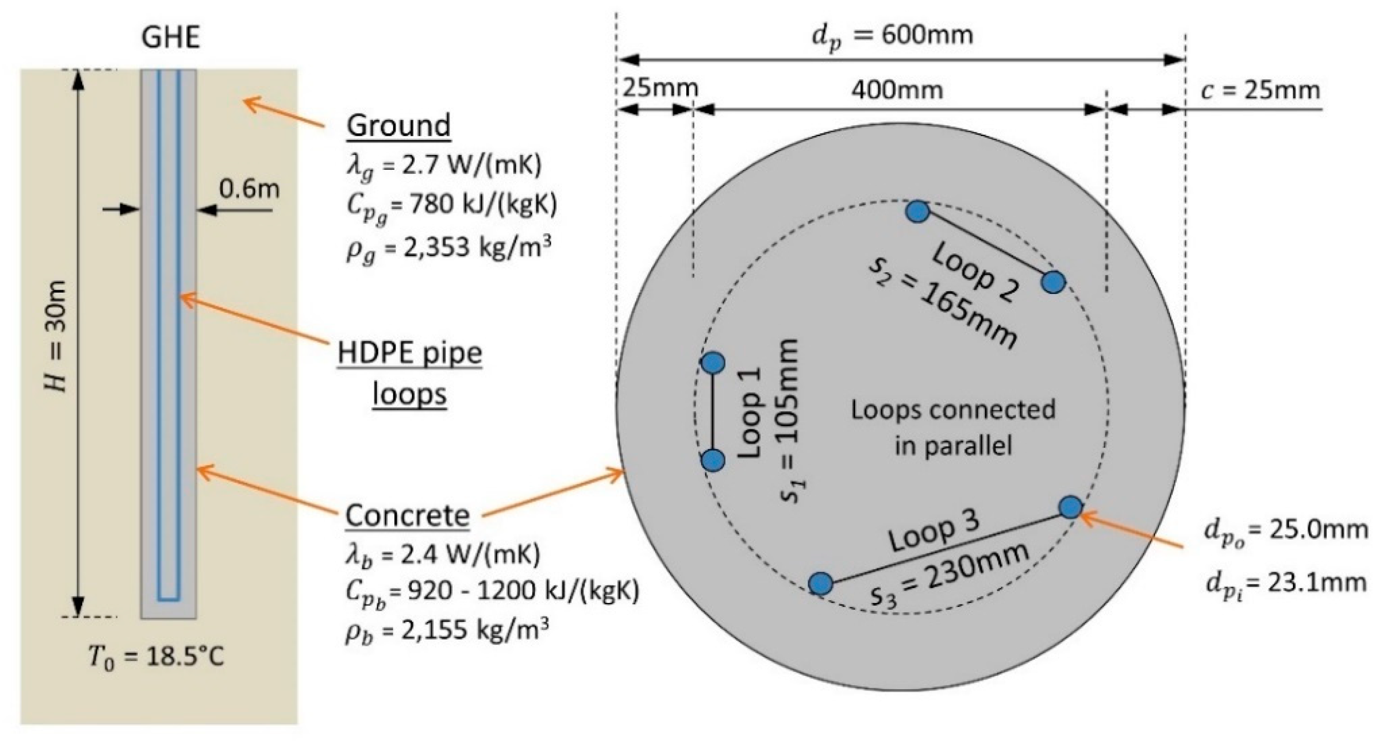
3.2. Test Site Details

The tested pile GHE is part of the Beaurepaire Centre shallow geothermal testing facility at the Parkville campus of the University of Melbourne, Australia. Detailed descriptions of the site, test pile construction, and previous thermal test history can be found in Colls et al. [44] and in Colls [45]. The geology at the location is Melbourne Formation residual clay overlaying siltstone and sandstone [46]. The groundwater table is approximately 13 m deep with no evidence of significant groundwater flow. The Pile GHE comprises three U-loops (L1, L2, and L3) at unequal separation connected in parallel (Figure 1), with geometrical characteristics summarised in Table 1. The table also contains thermal property estimates based on previous laboratory and in-situ testing at the site. These are used as initial values for the subsequent parameter estimation process.

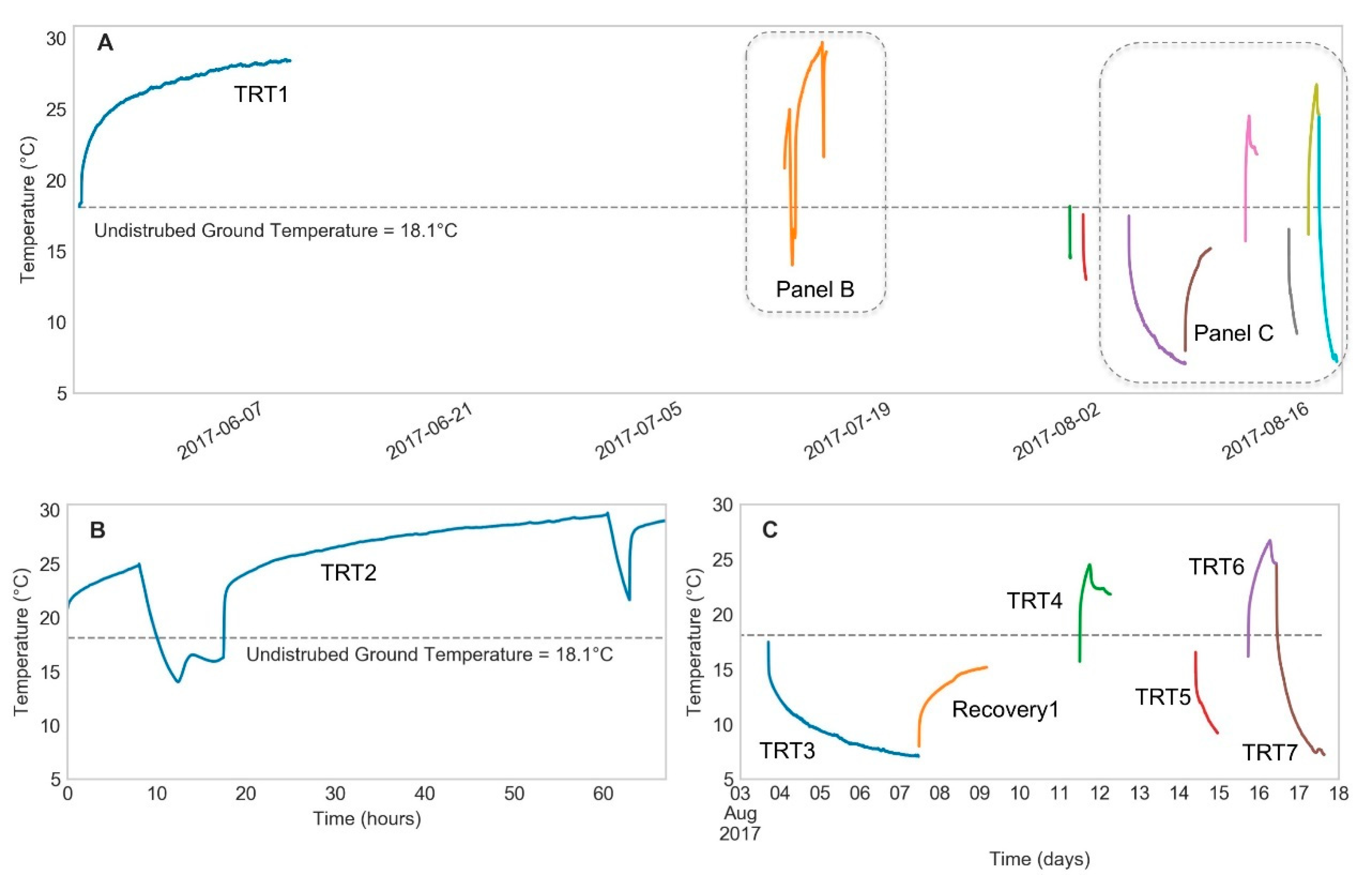
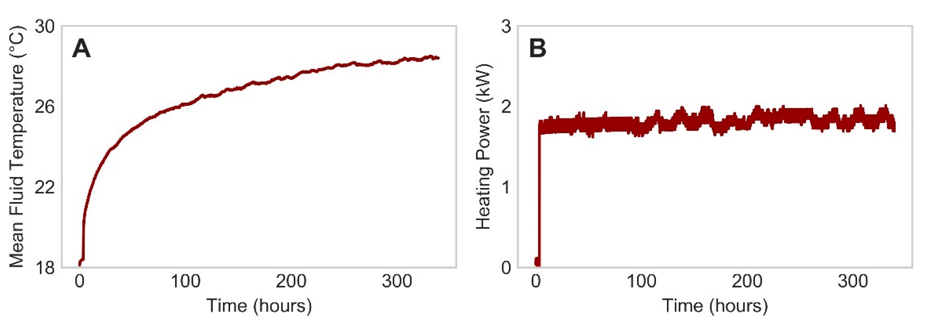
3.3. Pile TRT Field Trials

Seven separate TRTs were conducted on the pile during this study. Figure 2A shows the mean fluid temperature (solid line) for all tests, along with the undisturbed ground temperature (dashed line) of 18.1 °C. The latter was determined by the method of Gehlin and Nordell [49] based on 3 h of fluid circulation prior to the first period of heat injection (TRT1). Figure 2B shows TRT2 and the effects of power failure in greater detail, while Figure 2C zooms in on TRTs 3 through 7, including one recorded ground temperature natural recovery period. Subsequent TRTs after the first test show lower initial fluid temperatures, which is due to the decreasing temperature of the water supply used to fill the TRT over the three months of winter.
Two TRT rigs were used, a Geocube (Precision Geothermal LLC, MN, U.S.A.) and a heat pump based TRT that allowed heating and cooling of the pile. TRT1 and TRT2 were conducted with the Geocube, while all other tests were conducted with the heat pump. The Geocube applies power directly via electric heating elements, while the heat pump TRT applies power by maintaining a constant temperature difference between the inlet and outlet pipes of the TRT and constant flow rate. For all tests each loop in the pile was connected in parallel and the applied heating power and flow rate assumed to be equally divided between the 3 loops ( F l o o p = 0.25 L/s = 15 L/min).
Table 2 summarizes the details of each TRT. A number of the tests suffered from excess power fluctuations and there were also two failed attempts at TRT3 (first cooling test). Given these difficulties and the fact that only the first test ran long enough to potentially reach a steady state, TRT1 has been used for the back calculation of thermal parameters via fitting of a numerical model to the data (Section 4.1.1). The remaining six TRT datasets were used for validation of the numerical model via forward simulation (Section 4.1.2).
Figure 3 shows the mean fluid temperature recorded during TRT1, along with the applied heating power. The power was calculated according to the temperature difference between inlet and outlet pipes and the mass flow rate and specific heat capacity of the fluid. The test ran for 14 days with a heating power of 1.8 kW or 60 W/m. The total power applied is less than for routine tests on deeper boreholes. This was to ensure that over the longer test duration the fluid did not heat up beyond safe levels for the pipe and TRT materials. While the applied power is fairly constant around a mean value, cyclic variation is evident and is due to the fluctuations in daily temperature along with daily fluctuations in the voltage of the power supply. This results in a standard deviation around the mean of 3.2% and up to 11% variation for the peaks, which according to the American Society of Heating, Refrigerating and Air-Conditioning Engineers ASHRAE [50] should be no more than 2% and 10%, respectively. Thus, the test may have increased uncertainty. The impact that this level of variation in the power supply has on analysis will be discussed in detail in Section 4.2.

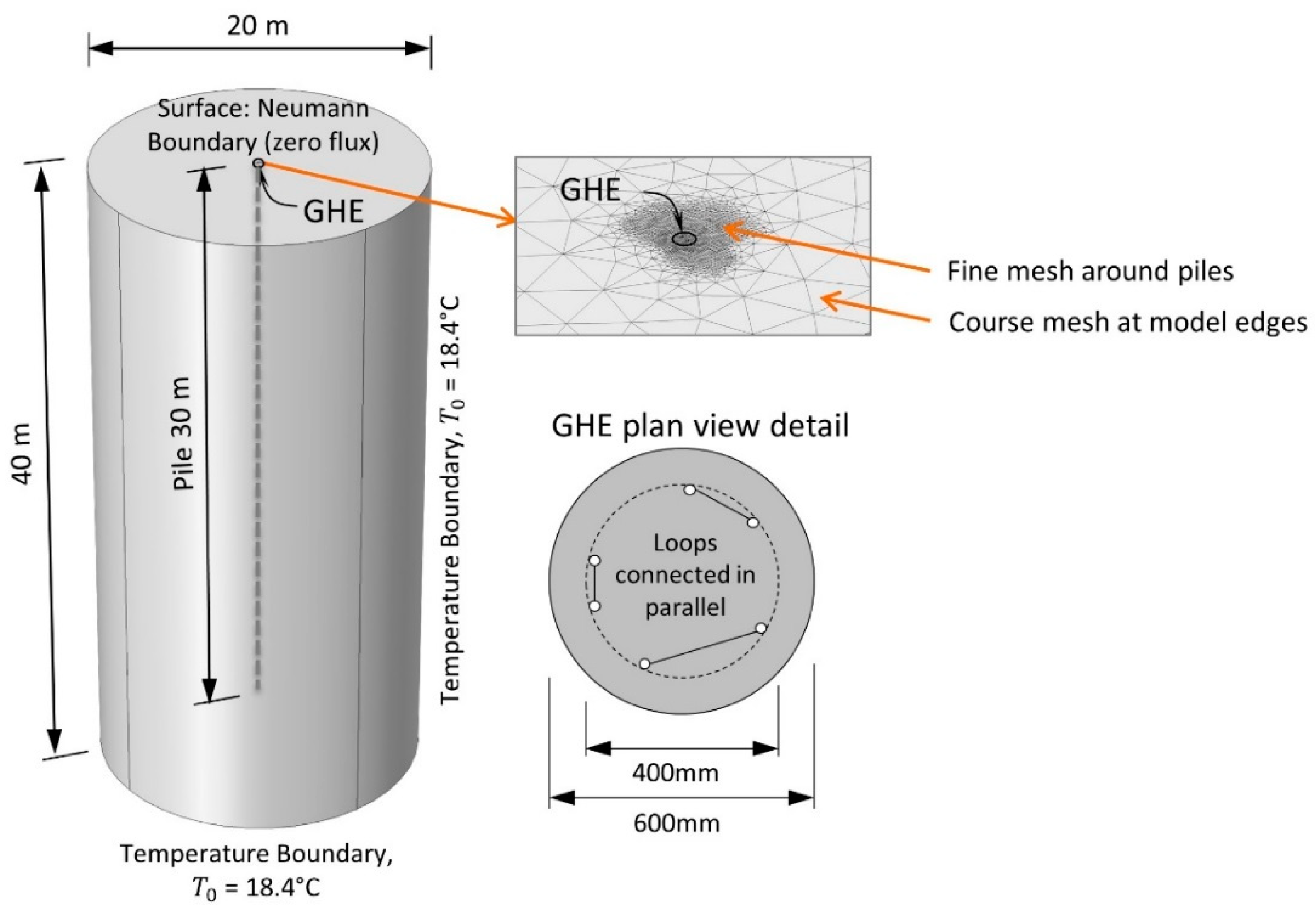
3.4. 3D Finite Element Analysis

A validated transient numerical model developed at the University of Melbourne is used [51,52,53]. The model is built and solved using the finite element software package COMSOL Multiphysics. A summary of the model is included in the following sections.

3.4.1. Model Description

The model is based on the coupling of the governing equations of heat transfer (energy balance) and fluid flow (momentum and continuity). It considers conduction in the ground, the concrete, and the pipe walls and partially in the fluid, and convection in the carrier fluid (groundwater flow is considered negligible at the case study site). For the fluid flow in the pipes, the continuity and momentum equations for (an incompressible) fluid and are solved [54]:
A ρ f · v = 0
ρ f ( v t ) = p f D ρ f 2 d h v | v |
where A is the inner cross-section of the HDPE pipe (m2), ρ f is the carrier fluid density (kg/m3), v represents the fluid velocity vector field (m/s), t shows the time (s), p is the pressure (Pa), f D represents the Darcy friction factor, and d h is the hydraulic diameter of the pipe. The energy equation for the fluid flow to describe the convective-conductive heat transfer for an incompressible fluid is [55]:
ρ f A C p f   T t + ρ f A C p f v ·   T = · ( A λ f T ) + f D ρ f A 2 d h | v | v 2 + Q w a l l
Q w a l l = f ( T p i p e   w a l l , T , λ p , d p )
where C p f is the specific heat capacity of the fluid (J/(kgK)), λ f represent thermal conductivity of the fluid (W/(mK)) and Q w a l l is the external heat exchange rate through the pipe wall (W/m). Here Q w a l l is a function of the temperature of the pipe outer wall T p i p e   w a l l , the temperature of the carrier fluid T , the pipe thermal conductivity λ p , and diameter d p [51,53]. The above equations are solved for pressure p , velocity field v and temperature field T in the carrier fluid and are coupled to the temperature field T m obtained from the conductive heat transfer equations solved for the surrounding concrete and ground by:
ρ m C p m T m t = · ( λ m T m )
where ρ m represents the solid material density (either concrete or the ground in this case), and C p m and λ m represent specific heat capacity and thermal conductivity of that solid material, respectively. Initial input parameters used in the model are as per Table 1. The λ and C p values for the ground and the concrete were then varied to obtain the best fit.
As the model does not present planes of symmetry a full 3D mesh is developed to capture the geometry in Figure 1. The model comprised approximately 420,000 elements with a minimum size of 0.02 m. Mesh refinement was carried out around the pipes and pile and a sensitivity analysis conducted as part of the parameter estimation exercise, with results given in Section 4.1.

3.4.2. Initial and Boundary Conditions

To solve the above systems of partial differential equations, initial and boundary conditions must be specified. The initial ground, pile and farfield boundary temperatures are set to be equal to the undisturbed ground temperature measured at the site as part of this study, where T 0 = 18.1 °C.
The time dependent carrier fluid temperature at the inlet T i n ( t ) , is defined as a function of the thermal power provided by the TRT unit Q and the fluid temperature at the outlet T o u t ( t ) , obtained from solving the numerical model. This is effectively acting as the transfer function of the TRT unit that receives the fluid at certain temperature ( T o u t ( t ) ) and extracts/rejects heat, changing the temperature of the fluid that is reinjected to the ground ( T i n ( t ) ) as in:
T i n ( t ) = T o u t ( t ) + ( Q / ( ρ f v A C p f ) )
where ρ f is the carrier fluid density and v represents the average fluid velocity. A fluid flow rate boundary condition at each inlet pipe of the three loops of 0.25 L/s (15 L/min) was applied resulting in an initial pipe velocity of v 0 = 0.7 m/s, along with a reference atmospheric pressure in the outlet pipes of p 0 = 101 kPa for the purpose of forced convection.
For the parameter estimation simulation, the time varying power input as per Figure 3B was applied in 2-min time steps. For the generation of synthetic TRT data, all other modelling parameters and boundary conditions were unchanged, except Q , which was set to a constant value equal to 1.81 kW (the average of the time series field data).
Finally, a zero heat flux boundary condition at the top surface is prescribed:
n · ( λ m T ) = 0
Given the relatively short (days) duration of the test, thermal solar recharge is neglected for simplicity. The model geometry, extent and boundary conditions are shown in Figure 4.

3.5. Analytical Models for GHE Temperature Response

A key factor in the usefulness of borehole TRTs is that the data can easily be interpreted with simple analytical heat transfer models. The common analytical models available include the ILSM (introduced in Section 2.2), the Infinite Cylindrical Source Model (ICSM), and the Finite Line Source Model (FLSM). As the names suggest, each model makes significant simplifying assumptions on the geometry, either being infinitely long or a line source of heat. A transient analytical pile model was also tested [6]. All models assume homogeneous and isotropic conditions.

3.5.1. Steady State Models

The three common analytical models mentioned rely on the presence of a quasi-thermal steady state within the GHE (i.e., R b is assumed constant). This includes the ILSM (Section 2.2), where further simplification of Equation (1) [29] allows ground thermal conductivity to be simply determined from:
λ g = Q 4 π m H
where m is the slope of the graph of mean fluid temperature against the natural logarithm of time. The GHE thermal resistance R b can then be evaluated from the same fitted line at T ( t 1 h r ) , which is conveniently the intercept in l n -space [29]:
R b = 1 4 π λ g [ T ( t 1 h r ) T 0 m l n ( 4 α g t 1 h r γ r b 2 ) ]
Additionally, Equation (1) for the ILSM and its full form (Equation (2)) have been used directly; applying parameter estimation to determine λ g and R b simultaneously rather than separately via Equations (12) and (13).
The second model is the ICSM, which assumes that the GHE acts as a hollow cylinder with a finite radius, and is based on the concept of a G-function, which is a dimensionless temperature response depending on the Fourier number and dimensionless radius [28,56,57]. The full ICSM formulation is:
T = Q H [ R b + F s c λ s G ( F 0 , 1 ) ] + T 0
where the G-function is:
G ( F 0 , 1 ) = 1 π 2 0 e β 2 F 0 1 J 1 2 ( β ) + Y 1 2 ( β ) [ J 0 ( β ) Y 1 ( β ) J 1 ( β ) Y 0 ( β ) ] d β β 2
In Equation (15), J 0 ( β ) , J 1 ( β ) ,   Y 0 ( β ) , and Y 1 ( β ) are Bessel functions, F 0 is the Fourier number, and F s c is a short-circuit heat loss factor. In this study the Bessel functions in the ICSM were solved numerically with built in functions in the python language scientific computing library SciPy [58].
The third model, the FLSM, is an analytical solution to Eskilson’s [31] model, first presented by Zeng et al. [59,60]. It differs from the ILSM by giving the temperature development at different depths (z) in addition to radial distances from the centre of the line source. It also accounts for the axial heat flow which is neglected in the ILSM and ICSM. In this work a simplified solution for the FLSM [61] has been applied due to faster computation time. The model determines the integral mean temperature along the GHE:
T f ( t , z ) = T 0 + Q H R b + Q 2 H λ g π [ β β 2 + 1 e r f c ( ω β ) z 2 β 2 d z D A β 2 + 1 β 2 + 4 e r f c ( ω β ) z 2 β 2 d z D B ]
where β = r b / H , ω = H / 4 α g t , and e r f c is the complimentary error function. The analytical expansions D A and D B are:
D A = β 2 + 1 e r f c ( ω β 2 + 1 ) β e r f c ( ω β ) ( e ω 2 ( β 2 + 1 ) e ω 2 β 2 ω π )
D B = β 2 + 1 e r f c ( ω β 2 + 1 ) 0.5 ( β e r f c ( ω β ) + β 2 + 4 e r f c ( ω β 2 + 4 ) ) ( e ω 2 ( β 2 + 1 ) 0.5 ( e ω 2 β 2 + e ω 2 ( β 2 + 4 ) ) ω π )

3.5.2. Transient Pile Models

A fourth analytical model was implemented with empirical transient G-functions for the ground and concrete which was developed specifically for piles [6]. Sets of upper and lower bound solutions based on numerical modelling of a range of pile geometries were used to generate curve fitting derived G-functions that can model the thermal response of a single pile. Compared to the steady state methods above, this approach accounts for both the transient conduction within the pile and an explicit pile geometry. Axial heat conduction is also included similarly to the FLSM. The equation for the fluid temperature in the pile is given as:
Δ T f = Q H R p + Q H R c G c + Q 2 π H λ g G g
where R p is the thermal resistance of the pipes (see Section 2.3), G c is the concrete G-function describing the transient concrete response and G g is the pile G-function for the transient response of the ground surrounding the piles. Sets of coefficients are provided in Loveridge and Powrie [6] for the two G-functions corresponding to different aspect ratios ( A R ) for G g and whether the pipes are located near the centre or the edge of the pile for G c . Results based on Equation (19) presented in this study are for lower bound G-functions for both G g and G c , assuming A R = 50 and pipes near the pile edge, since these provide the best match to the geometry and properties of the 600 mm pile in this study.

3.5.3. Implementation

In all cases, except for separate determination of λ g and R b using the ILSM (Equations (12) and (13)), the analytical models were fitted using an automated parameter estimation process based on the Limited Memory BFGS (Broyden–Fletcher–Goldfarb–Shanno) algorithm with bound constraints from the python package SciPy [58]. A two-parameter curve fitting scheme was used to find the λ g and R b , with all other thermal parameters (i.e., C p v g ) kept constant (see Table 1).

4. Results

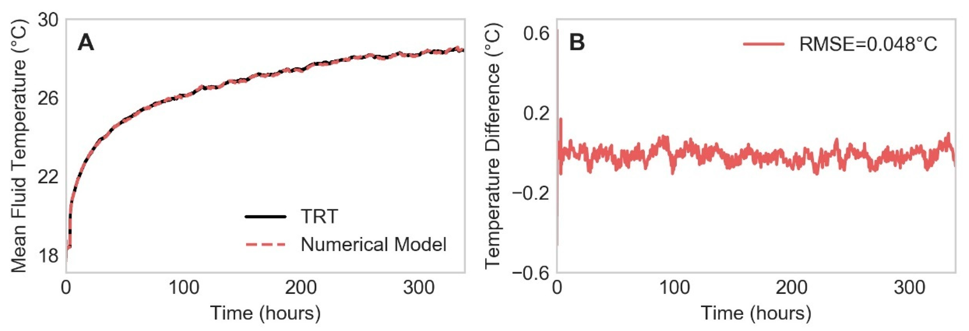
4.1. Numerical Simulation

4.1.1. Parameter Estimation of Ground Properties

The numerical model was validated and key ground and concrete thermal parameters found by fitting to the TRT1 dataset. A parameter estimation scheme was used to find a combination of λ g , λ c , C p v g , and C p v c that produced the minimum Root Mean Squared Error (RMSE) fit to the experimental data. Figure 5A shows the numerically simulated TRT based on best-fit parameters compared to the experimental data, and Figure 5B shows the residuals confirming a close fit with an RMSE of 0.048 °C. A mesh sensitivity analysis was conducted that resulted in only a 0.002 °C reduction in RMSE by increasing the mesh size from approximately 350,000 elements to 420,000, indicating that the results presented in this study are mesh independent.
Table 3 compares the parameter estimation results with the results from previous laboratory and in-situ studies at the site indicating good agreement. The high quality of fit and the close correspondence of the results to independent measurements suggests that the numerical model is capable of accurately simulating the thermal processes in the pile and ground during a TRT. Conducting a TRT on a pile can thus provide excellent evaluation of thermal parameters if 3D numerical parameter estimation is carried out. However, relying on a numerical model requires designers to have access to advanced finite element software and the expertise to use it, while also necessitating long computation times, making the approach impractical for routine implementation. In this case, each iteration of the numerical simulation took approximately 3.5 h on a high-performance desktop computer with eight 3.4 GHz processors and 16 GB of RAM. Finding the best fit solution shown above required over 50 iterations with a total computation time of over one week, excluding model set up and mesh validation. Hence, 3D simulation is likely to remain an academic interpretation tool for some time.

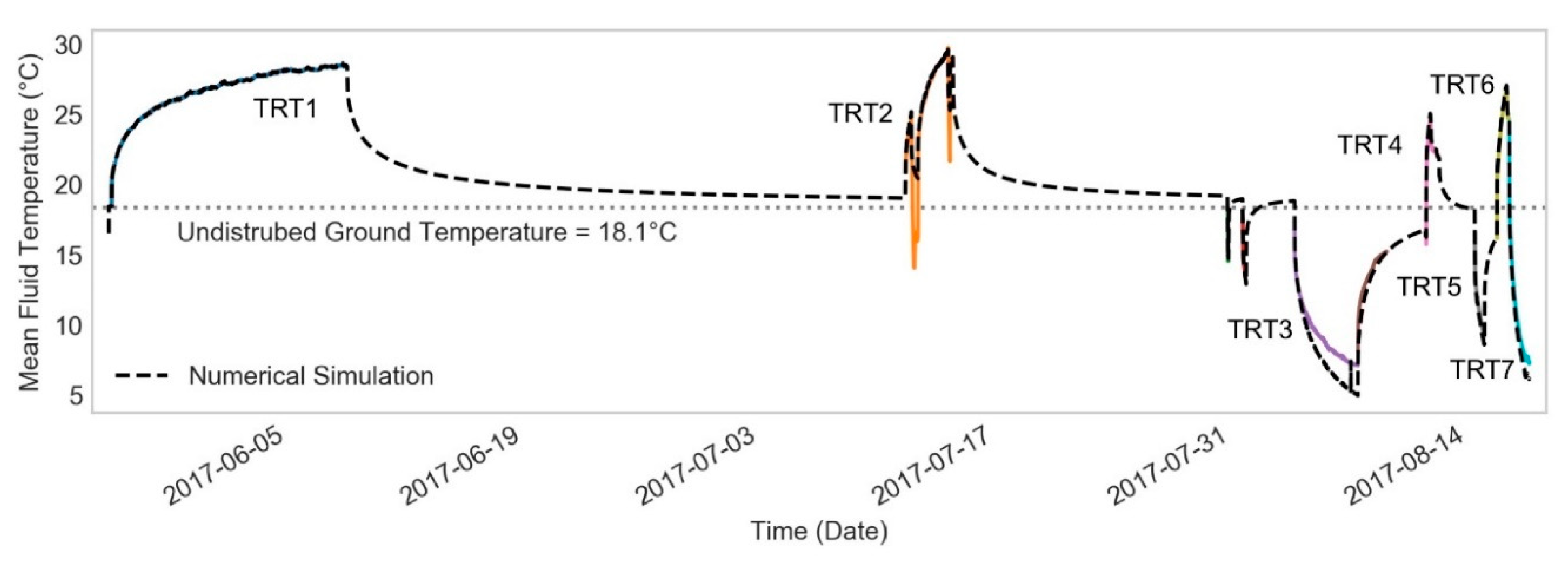
4.1.2. Forward Simulation

The validated numerical model was used for forward prediction of the remaining TRT datasets (Figure 2). This helps to determine whether there was bias in the selection and use of the parameters found by curve fitting, and also whether the model can be used to simulate conditions that differ from those of TRT1. Furthermore, this process provides a check that no hysteric behaviour is occurring; i.e., that the temperature changes are fully reversible with no changes in the thermal parameters.
Since each subsequent test is affected by the previous one, a long-term simulation was run to cover all tests in sequence including the rest periods as shown in Figure 6. The RMSEs of the tests indicating the quality of the numerical simulations are given in Table 4. After TRT1, the numerical model was not able to replicate the measured data with the same accuracy, although the model certainly captures the general trend of each TRT. With the exception of TRT3 (cooling) and the power outages in TRT2, the temperature peaks are mostly well reproduced (Figure 7). Most importantly, the quality of the fit does not get systematically worse throughout the tests, suggesting that hysteresis of behaviour is probably not occurring. However, the model does appear less able to accurately simulate the cooling test periods compared to the heating periods, particularly for TRT3. For TRT2, the periods of power outage over night show a significant ambient temperature signal, which the model was not able to account for, resulting in much lower temperatures during these periods than the model results and leading to the highest RMSE. Nonetheless, the forward simulation helps to confirm that the thermal parameters established from fitting to TRT1 are an appropriate overall representation of actual site conditions. Section 4.1.3 Estimation of steady state thermal resistance.

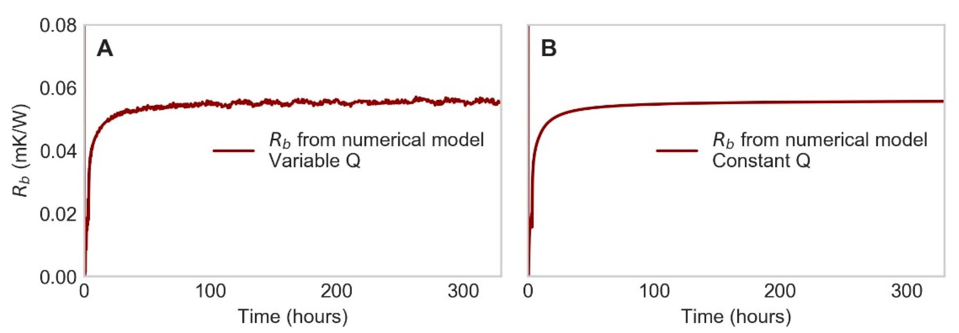
4.1.3. Estimation of Steady State Thermal Resistance

The use of classical analytical solutions (ILSM, ICSM, and FLSM) relies on the assumption of a thermal steady state within the GHE. Figure 7A shows R b calculated from the best fit numerical model solution presented in Table 4 using Equation (4). While R b approaches a constant steady state value around 100 h, it is never truly constant. This is due to the applied power variation (Figure 3). Each time the power changes, the concrete becomes transient again immediately adjacent to the pipes, hence the corresponding R b fluctuations. Figure 7B shows the same calculation for a constant power synthetic TRT dataset generated from the numerical model. From this result it can be seen that R b converges to a value of 0.056 mK/W.
Taking the data from Figure 7B, and by assuming a steady state value of 0.056 mK/W, the time to steady state can be confirmed. 98% of steady state is reached after 87 h of the test, which corresponds to the benchmark Fourier Number F o 5. By F o 10, which corresponds to 173 h, 99.3% steady state R b is reached, agreeing with the observations for pile thermal resistance presented in Loveridge and Powrie [6]. Thus, the industry accepted standard of F o 5 as the start of the steady state for borehole TRTs appears also to be applicable to piles. The difference is that instead of this early time criterion being a few hours for typical borehole geometries, for piles this could be several days.

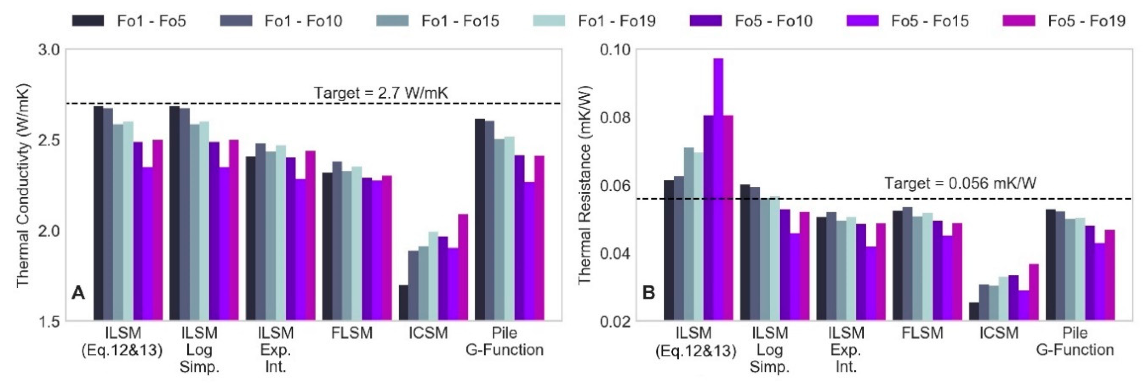
4.2. Application of Analytical Models

4.2.1. Experimental Data

The analytical models described in Section 3.5, ILSM, FLSM, ICSM, and Transient Pile Models, have been fitted to the experimental TRT data to estimate the thermal parameters λ g and R b . Note that estimates from three implementation variations of the ILSM are included: (i) using Equations (12) and (13) and the m and the y-intercept found from linear regressions in the T(t) versus ln(t) plots (ILSM-Eq. 12&13), (ii) best fits using the simplified Equation (1) (ILSM–Log Simp.), and (iii) best fits using Equation (2), the full version of the analytical solution to the heat diffusion equation (ILSM–Exp. Int.). Figure 8 compares these analytical results to the target values determined from numerical simulation (black dashed lines). The analytical models have been fitted to periods in the field data bounded by five distinct time points: F o 1, 5, 10, 15, and 19.4 (end of test), which correspond to 17, 87, 173, 260, and 336 h, respectively. The fitting regions starting from F o 1 include the early time, non-steady state region, while the regions starting at F o 5 fall within a steady state (Section 4.1.3).
With the exception of the ICSM, the λ g estimates from all fitting windows fall within 15% of the target value. For R b , the difference between the target values and analytical results show the same pattern as for λ g , except for the ILSM with linear regression (Equations (12) and (13)) which overestimates the target value significantly. More importantly, most of the models show reduced accuracy where later periods of the test are included in the analysis (up to F o 15 or 19.4), and when the fitting region starts later at F o 5 instead of 1. This is contrary to expectation of longer tests providing greater accuracy. Therefore, it suggests that late time data has reduced quality compared to the early time data, which is most likely due to noise and high frequency fluctuations of the experimental data. The ILSM variations also all under-predict the thermal conductivity when an overestimate would have been expected [30].
To explore the variation in results with test time in more detail, a step-wise analysis was carried out [62]. The three ILSM implementations are shown as examples. Transient estimates of λ g (Figure 9A) and R b (Figure 9B) were made from consecutive 100 h sub-samples of the temperature curve using a sliding window approach and fitting the three ILSM models to each window. The start times of each window were increased 1 h and are the values on the x-axis.
The estimates vary considerably depending on the fitting window and by up to 50% from the minimum to maximum values. Additionally, the simplest ILSM (Equations (12) and (13)) gives significantly different results in terms of R b in the middle of the test compared to the other two models, suggesting that y-intercept approach (Equation (13)) may not be suited for returning realistic values from pile TRT data. Generally, stability in terms of λ g and R b reduces as the test progresses. The most consistent results are from fitting windows starting from between 0 and 100 h, with start times after this leading to larger variations from the target value. This suggests that noise has an increasing impact at later times in the pile TRT, leading to the concept that a signal to noise ratio (SNR) plays a role in the level of uncertainty. The noise is generated by fluctuations in the applied power, which increase in relative significance later in the test when the absolute rate of change of temperature is smaller. Figure 10 shows an estimate of SNR for TRT1 data over sucessive time windows of 24 h. Here, we define SNR = m / s t d , where m is the linear rate of change of temperature over the time window and s t d is the standard deviation of the distribution of temperature measurements over that same time window. There is an increase in variability caused by fluctuations in the temperature response, which have a clear cyclic amplitude of approximately 24 h matching diurnal temperature change. This variablity increases as the test progresses and the overall SNR decreases towards the end of the test. Both Figure 9 and Figure 10 indicate significantly increased variability after approximately 100 h for TRT1, thus explaining why the analytical model results shown in Figure 8 offer a worse fit when using later time data.
In fact, this concept of SNR may lead to an upper limit on the useful test length of large diameter pile TRTs. Longer test times are needed than for boreholes to reach a steady state condition, but at the same time must use low heating power to ensure that the pile, fluid, and TRT rig do not reach damaging temperatures over the course of a potentially several week test. This low heating power will make pile TRTs more susceptible to errors resulting from decreasing SNR over the course of the test. Thus, it may be challenging to conduct TRTs on large diameter piles with high quality results.

4.2.2. Synthetic TRT Data

The uncertainties arising from the low SNR makes an assessment between the relative performance of the different analytical models difficult. Therefore, a synthetic TRT from the best fit model with constant heating power of 1.81 kW (average of the experimental power measurements) was produced to permit clearer comparisons.
Fitting of the analytical models was repeated for this new dataset and is shown in Figure 11. The same time windows were used for the analysis as with the original TRT1 data (Figure 8). Comparable step-wise analysis was also carried out (Figure 12). The results are now more as expected and the model fit tends to improve with time. The simplest ILSM (Equations (12) and (13)) and two-parameter curve fitting produce the same estimates of λ g , and give results close to the target of 2.7 W/(mK) over a range of time windows. The ILSM with Ei() accounts more for the transition between the lower concrete thermal conductivity (2.5 W/(mK)) and the higher ground thermal conductivity. For R b , the ILSM with Ei() returns values closest to the expected value of 0.056 (mK/W) based on the numerical results, whereas the other ILSM models over estimate R b , and the ICSM, FLSM, and Pile G-function models underestimate R b .
Amongst the models shown in Figure 11, the ICSM produces much more conservative results, underestimating λ g and R b by around 10% and 20%, respectively. This is consistent with the ICSM having a lower gradient compared to the ILSM at the timescales of interest to a TRT. This poor performance is consistent with previous work suggesting the ICSM to be inappropriate for piles [6]. The FLSM also underestimates λ g and R b . This is because it produces lower temperatures over the same time region than the ILSM due to axial effects. Despite the FLSM providing worse estimates of the thermal properties compared with the ILSM, it shows the best overall fit (Figure 13). This may reflect the co-linearity of the λ g and R b and the fact that the corresponding errors in each may cancel each other out.
Overall, the best performing steady state model is the ILSM. The log-linear versions appear to perform well over a range of timescales, but this may not be a general conclusion since the concrete and ground thermal conductivities are close in this case. These models also do not give as good a prediction of R b . On the other hand, the full exponential integral derivation of the ILSM captures λ c = 2.5 W/(mK) at the early time ( F o 1–5), λ g = 2.62 (~2.7) W/(mK) in the late time ( F o 5–19.4), and R b closest to the steady state value of 0.056 mK/W in the late time. However, the reliance on the late time data to give appropriate predictions means that the accuracy of this model will be dependent on achieving high SNR late in the test, and can be seen in Figure 8 to produce less accurate results than other models when the data is noisy.
The pile G-function approach with lower bounds performs similarly to the ILSM in terms of accuracy but does this from assessment of the early time transient data. It gives a slight underestimation of λ g , which is consistent with another test on smaller energy piles by Alberdi-Pagola et al. [36], but most importantly gives good results from fitting to the early time, even for the region of F o 1–5. The G-function approach explicitly treats the pile and ground thermal conductivity separately and models the early time transient behavior. Thus, these results suggest shorter tests times that lead to accurate estimation of ground thermal conductivity can be achieved with the G-function model with lower bounds, while overcoming the issues related to higher uncertainty in late time data due to noise and high frequency fluctuations. The G-function approach is also the only model to provide a good fit to the synthetic TRT dataset from the 1st hour onwards based on this early time fit, as shown in Figure 13. The ICSM fit shown in Figure 13 also demonstrates why this model produces the worst results, since the model is not able to fit the shape of the measured data until after 200 h.

4.3. Alternative Determination of Thermal Resistance

Because of the difficulties relating to pile thermal response testing, including long durations, and hence high costs, it may be desirable to obtain pile parameters by other means. There are realistically few methods available and all will require knowledge of concrete thermal conductivity. Methods based on numerical simulation additionally require knowledge of concrete specific heat. In this case, these values are known reliably from the parameter estimation exercise, although this may not always be the case. Alternate estimates of the pile thermal resistance are summarized in Table 5. While the empirical 2D resistance approach overestimates the pile thermal resistance, the multipole method [42] produces the closest value to the numerically estimated R b . Guidance based on the multipole method in Pahud [24] has overestimated R b in this case, presumably because of the high concrete thermal conductivity in this particular pile compared to the 1.8 W/(mK) assumed by the authors. The multipole method is generally considered the best theoretical approach for estimating R b [43] and appears to also perform well in this case of a large diameter pile with three loops. Therefore, it seems reasonable to assume that accurate estimates of pile R b may be made independently without the need for a pile TRT, as long as the concrete thermal properties can be reliably measured through samples or some other means.

5. Discussion: Viability of Pile TRTs

In the sections below, the viability of pile TRTs in assessed by reference to practical and technical considerations, with a summary given at the end in Table 6.

5.1. Testing Time

Based on the steady state analysis shown in Section 4.2, it seems that the industry accepted minimum test time of F o 5 still holds for a pile geometry if steady state analytical analysis is desired. A period of testing is required after this to ensure enough steady state region is captured, which was previously suggested to be up to around F o 10, after which axial effects may start to impact on analytical results [6]. From this study, an upper limit of F o 10 (173 h) based on the increasing uncertainty due to reducing SNR also seems important, although an earlier cut off could be appropriate for poorer quality data. If the total testing time required for a pile TRT is up to F o 10, this will generally be much longer than the 48 h recommended for borehole TRTs, and could be several weeks for large diameter piles. Thus, greater costs in terms of labour, generator hire, and materials (see below) will be incurred, making pile TRTs unattractive for practical use on projects. However, there is the potential to reduce testing times based on a transient method of interpretation as discussed in the next section.

5.2. Interpretation Methods

The results in Table 3 show that use of a numerical model for analysis of pile TRT data is accurate and robust. However, the time required, the use of costly specialized software, and the skill involved make numerical interpretation of pile TRTs impractical for routine application in industry.
Of the steady state analytical methods tested, the ILSM with Exponential Integral potentially gives the most useful estimates of λ g and R b providing a long enough test is carried out. The change between the concrete and ground thermal conductivities appears to be captured depending on how much of the early time data is assessed. This model also gives the closest estimates of λ g and R b to the independent estimates based on the synthetic TRT data in Figure 11.
The Pile G-function model proposed by Loveridge and Powrie [6] also gives good results for λ g , with the closest to independent thermal parameter estimates achieved from the early time part of the data. This is an important distinction compared to the ILSM with Exponential Integral, since the G-function approach gives good results independent of the testing period, suggesting that a transient analysis approach can reduce the test time required for pile TRTs. However, greater errors do occur when determining R b . For all analytical methods, acceptable accuracy depends of achieving a good (high) SNR (ASHRAE standards absolute minimum requirement).

5.3. Construction Programme Implications

Pile construction is typically on the critical path for construction projects. Hence, carrying out a TRT on a working pile can influence the construction programme and overall costs. Time is first required for the pile heat of hydration to be fully dissipated. In this study, pile temperatures recorded during concrete curing reached nearly 70 °C a day after pouring, reducing to around 20 °C after 10 days [45]. This is still 1.5 to 2.0 °C above the undisturbed conditions and it is expected that the pile may have taken over a month to fully return to the undisturbed condition. Larger piles would require a longer time to restore thermal equilibrium. Loveridge and Powrie [63] reported a 1200 mm diameter energy pile taking over two months to cool following curing. Then, one to three weeks would be required for the TRT itself, giving substantial additional programme requirements all together. It is therefore recommended that a pile designated for TRT should be among the first constructed, maximising the time available for curing and testing before foundation construction advances to the next stage.
Some of these delays can be avoided on projects large enough to include a test pile, since this could be used for TRT applications as well as traditional load testing, potentially removing this activity from the critical path.

5.4. Pile versus Borehole Testing

Typically, the target information for design of the shallow geothermal system is the ground thermal conductivity, GHE thermal resistance, and the undisturbed ground temperature. Focusing on the ground parameters, a borehole TRT may be sufficient to provide this information. In particular, given the much shorter testing time and that a test borehole GHE could be constructed and tested off the critical path, this may be a more economical and lower risk option. However, depending on the time in the project when the test is constructed, the finished depth of the pile GHEs may not be finalised, and so a test borehole GHE could conceivably be drilled to an inappropriate depth, providing effective thermal conductivity estimates that are not representative of the ground around the thermal pile foundations. One solution to this challenge could be the use of distributed TRTs [30,64,65] where information is obtained as a function of depth. However, these are more expensive than traditional tests and are not yet routine in practice.
Borehole TRTs also do not provide any information about the pile thermal characteristics, so these would need to be determined separately. As discussed in Section 2.3 and Section 4.3, easily implemented methods to estimate R b accurately are not necessarily available. Numerical simulation or the multi-pole method appear to be the most accurate methods, but both require high skill levels to implement. They also require an independent estimate of the pile thermal properties, which would necessitate taking of concrete samples during construction for subsequent laboratory testing. Laboratory thermal conductivity testing can have its own pitfalls [30], and a key source of uncertainty in this respect would be lack of knowledge about the final moisture condition of the concrete in the ground. Table 6 summarizes the main different approaches available.

5.5. Cost Analysis

For the cases in Table 6, a cost analysis has been conducted. The costs assigned to the components are based on data reported in Lu et al. [66] and a borehole/pile of 30 m depth, and are shown in Table 7. Costs are given in Australian Dollars based on current market conditions. While the cost of utilizing an existing site investigation borehole is minimal, the final energy pile design length may not be finalized, and the length of the test borehole may not match. This means there is an information gain moving from this to a bespoke borehole, and then again to a working pile. However, given the potential additional errors for pile TRTs if SNR is not controlled, greater value may not be realized in practice.

6. Recommendations

6.1. Pile TRT Test Duration

Recommended test duration will depend on the analysis method to be adopted. Tests using steady state analytical models for interpretation should be extended to Fo10 and carried out with due regard to power fluctuations as discussed in Section 6.2 below. Longer duration tests are likely to have further reduced accuracy unless exceptional power control can be maintained.
Pile TRTs to be interpreted using transient methods, either analytical or numerical, can be reduced to Fo5.

6.2. Pile TRT Power Control

Control of power levels is important to limit the reduction in SNR over the course of the test. The ASHRAE power requirements (standard deviation no more than 2% of the mean, up to 10% variation for peaks) should be adhered to as a minimum standard for tests to Fo5, although exceedance of these standards would still be desirable.
Longer pile TRTs should significantly exceed ASHRAE standards, with an aim to keep data noise to a minimum. Best practice measures that can be taken include:
  • Use of a dedicated generator rather than fluctuating site electricity supply.
  • Carefully insulate the TRT casing and above ground piping, minimise surface piping lengths and attempt to keep the unit out of the sun and wind.
  • Apply the highest power possible that will not cause over heating at later times to maximise the SNR in the late time part of the test. Analytical models can be used to estimate the late time temperature to help choose a power level.
  • Where there is flexibility in running a heating (traditional) or cooling TRT, the difference between the initial ground temperature and the late time fluid temperature can be exploited to maximise the allowable temperature change over time. For example, if the ground temperature was 20+ °C, it may be beneficial to run a cooling test and target late time fluid temperatures around 3–4 °C instead of potentially overheating the pile with a heating test, as this maximises the temperature change in relation to maximising SNR.
  • Include a recovery period in the TRT, which generally gives a better estimate of R b [67] and will be less susceptible to noise effects. However, this will also increase the time and cost required for the test.

6.3. Borehole Tests

Where it is decided to test a borehole instead of a pile, the cost and benefit of using a bespoke borehole later in the project needs to be evaluated against using a site investigation borehole at the outset. Additionally, an alternative method needs to be used to determine the pile thermal resistance. This should be done either numerically (two dimensions would be sufficient [25]), or using the multipole method to get realistic results. To make the assessment of pile thermal resistance the concrete thermal conductivity would be required. This necessitates taking concrete samples during construction for laboratory testing. Dry and saturated samples should be tested, but judgement will be needed about the likely in-situ moisture conditions of the pile concrete during operation.

7. Conclusions

A long duration series of thermal response tests were carried out on a 600 mm diameter pile to investigate the applicability of the technique to large diameter energy piles. Numerical and analytical tools were used to interpret both the field data and additional numerically generated synthetic test data. Detailed analysis showed that:
  • 3D numerical simulation can provide a good match to the TRT test data, providing a reliable means of parameter estimation. Subsequent forward simulation suggests no heating-cooling hysteresis, although the fit to field data does reduce with complex thermal loading cycles.
  • Steady state analytical models can be used for interpretation of the test data, providing the test duration is at least F o 10.
  • However, for tests longer than F o 5, high signal to noise ratio in captured field data is essential, increasing the importance of controlling the power supply to the test. Power fluctuations significantly below those required by ASHRAE are recommended to avoid loss of accuracy. Combined with 2, this makes obtaining reliable soil and pile parameters challenging.
  • Alternatively, a transient analytical pile model was able to produce reliable estimates of λ g and R b from much earlier in the test. This could reduce testing times and hence costs, as well as avoid the difficulties of obtaining high SNR data.
  • Further cost savings can be obtained from testing a borehole on the same site and estimating the pile properties from other methods. However, consideration is required regarding the test borehole length and laboratory assessment for concrete thermal properties, both of which can add uncertainty to the results obtained.

Author Contributions

Conceptualization, F.L. and G.A.N.; methodology, L.J.-P., F.L., and G.A.N.; software, L.J.-P.; validation, L.J.-P.; formal analysis, L.J.-P.; investigation, L.J.-P.; resources, G.A.N.; data curation, L.J.-P.; writing—original draft preparation, L.J.-P. and F.L.; writing—review and editing, L.J.-P., F.L., and G.A.N.; visualization, L.J.-P.; supervision, G.A.N. and F.L.; project administration, G.A.N.; funding acquisition, G.A.N. and F.L.

Funding

The authors are grateful for support from the Department of Environment, Land, Water and Planning of the Government of Victoria (Sustainable Energy Pilot Demonstration (SEPD) Program). Fleur Loveridge was funded by the UK Royal Academy of Engineering and the Melbourne School of Engineering & IT Visiting Fellowship. Linden Jensen-Page was supported by the Len Stevens Scholarship. Guillermo Narsilio was funded by the Australian Research Council (FT140100227).

Acknowledgments

The authors would like to acknowledge the support provided by Melbourne University’s Sport Centre, and the Melbourne Energy Institute. The authors would also like to thank Saqib Javed from Chalmers University of Technology for the multipole method results.

Conflicts of Interest

The authors declare no conflict of interest. The funders had no role in the design of the study; in the collection, analyses, or interpretation of data; in the writing of the manuscript, or in the decision to publish the results.

Nomenclature

Main symbols used
αthermal diffusivity [m2/s]
γEuler’s constant
λthermal conductivity [W/(mK)]
ρdensity [kg/m3]
Across sectional area [m2]
cconcrete cover [m]
Cpspecific heat capacity [kJ/(kgK)]
ddiameter [m]
dhhydraulic diameter [m]
fDDarcy friction factor
Fflow rate [L/s]
FoFourier number
Fscshort circuit heat loss factor
GG-function
Hground heat exchanger length [m]
JBessel function
mgradient
ppressure [kPa]
qpower [W/m]
Qpower [W]
rradius [m]
Rresistance [mK/W]
sshank spacing [m]
ttime [s]
Ttemperature [°C or K]
vvelocity
YBessel function
Subscripts
0initial or undisturbed
bborehole or pile
cconcrete
condconductive
convconvective
ffluid
gground
iinner pipe dimension
ininlet
msolid material (in numerical model)
oouter pipe dimension
outoutlet
ppipes

References

  1. Australian Government. Australia’s 2030 Climate Change Target; Australian Government, Department of the Environment and Energy: Canberra, Australia, 2015.
  2. Bureau of Resources and Energy Economics. Australian Energy Update; Australian Government: Canberra, Australia, 2014.
  3. Lund, J.W.; Freeston, D.H.; Boyd, T.L. Direct utilization of geothermal energy 2010 worldwide review. Geothermics 2011, 40, 159–180. [Google Scholar] [CrossRef]
  4. Lund, J.W.; Boyd, T.L. Direct utilization of geothermal energy 2015 worldwide review. Geothermics 2016, 60, 66–93. [Google Scholar] [CrossRef]
  5. Brandl, H. Energy foundations and other thermo-active ground structures. Géotechnique 2006, 56, 81–122. [Google Scholar] [CrossRef]
  6. Loveridge, F.; Powrie, W. Temperature response functions (G-functions) for single pile heat exchangers. Energy 2013, 57, 554–564. [Google Scholar] [CrossRef]
  7. Bozis, D.; Papakostas, K.; Kyriakis, N. On the evaluation of design parameters effects on the heat transfer efficiency of energy piles. Energy Build. 2011, 43, 1020–1029. [Google Scholar] [CrossRef]
  8. Sekine, K.; Ooka, R.; Yokoi, M.; Shiba, Y.; Hwang, S. Development of a ground source heat pump system with ground heat exchanger utilizing the cast-in-place concrete pile foundations of a building. ASHRAE Trans. 2007, 113, 741–753. [Google Scholar]
  9. Park, S.; Sung, C.; Jung, K.; Sohn, B.; Chauchois, A.; Choi, H. Constructability and heat exchange efficiency of large diameter cast-in-place energy piles with various configurations of heat exchange pipe. Appl. Eng. 2015, 90, 1061–1071. [Google Scholar] [CrossRef]
  10. Lu, Q.; Narsilio, G.A. Economic analysis of utilising energy piles for residential buildings. Renew. Energy 2019. under review. [Google Scholar]
  11. Amis, A.; Loveridge, F.A. Energy piles and other thermal foundations for GSHP—developments in UK practice and research. REHVA J. 2014, 2014, 32–35. [Google Scholar]
  12. Austin, W.A., III. Development of an in Situ System for Measuring Ground Thermal Properties. Doctoral Thesis, Oklahoma State University, Stillwater, OK, USA, 1998. [Google Scholar]
  13. Gehlin, S.; Eklof, C. TED: A Mobile Equipment for Thermal Response Test. Master’s Thesis, Luleå University of Technology, Luleå, Sweden, 1996. [Google Scholar]
  14. VDI. VDI 4640 Blatt 3 Utilization of the Subsurface for Thermal Purposes; Underground Thermal Energy Storage; VDI-Gessellschaft Energie Und Umwelt (GEU): Berlin, Germany, 2001. [Google Scholar]
  15. Mikhaylova, O.; Johnston, I.W.; Narsilio, G.A. Uncertainties in the design of ground heat exchangers. Environ. Geotech. 2016, 3, 253–264. [Google Scholar] [CrossRef]
  16. Loveridge, F. The Thermal Performance of Foundation Piles Used as Heat Exchangers in Ground Energy Systems. Ph.D. Thesis, University of Southampton, Southampton, UK, 2012. [Google Scholar]
  17. Franco, A.; Moffat, R.; Toledo, M.; Herrera, P. Numerical sensitivity analysis of thermal response tests (TRT) in energy piles. Renew. Energy 2016, 86, 985–992. [Google Scholar] [CrossRef]
  18. GSHPA. Thermal Pile Design Installation and Materials Standards; Ground Source Heat Pump Association: Milt Keynes, UK, 2012. [Google Scholar]
  19. Hu, P.; Zha, J.; Lei, F.; Zhu, N.; Wu, T. A composite cylindrical model and its application in analysis of thermal response and performance for energy pile. Energy Build. 2014, 84, 324–332. [Google Scholar] [CrossRef]
  20. Loveridge, F.; Powrie, W.; Nicholson, D. Comparison of two different models for pile thermal response test interpretation. ACTA Geotech. 2014, 9, 367–384. [Google Scholar] [CrossRef] [Green Version]
  21. Loveridge, F.A.; Brettmann, T.; Olgun, C.G.; Powrie, W. Assessing the applicability of thermal response testing to energy piles. In Global Perspectives on the Sustainable Execution of Foundations Works; Infrastructure Group: Stockholm, Sweden, 2014; Volume 0044, p. 10. [Google Scholar]
  22. Badenes, B.; de Santiago, C.; Nope, F.; Magraner, T.; Urchueguia, J.F.; de Groot, M.; de Santayana, F.P.; Arcoset, J.L.; Martín, F. Thermal characterization of a geothermal precast pile in Valencia (Spain). In Proceedings of the European Geothermal Congress (EGC 2016), Strasbourg, France, 19–24 September 2016. [Google Scholar]
  23. Bourne-Webb, P.; Burlon, S.; Javed, S.; Kürten, S.; Loveridge, F.A. Analysis and design methods for energy geostructures. Renew. Sustain. Energy Rev. 2016, 65, 402–419. [Google Scholar] [CrossRef]
  24. Pahud, D. Simulation Tool for Heating/Cooling Systems with Heat Exchanger Piles or Boreholes Heat Exchangers; PileSim User’s Manual Swiss Fed Off Energy: Lausanne, Switzerland, 1999. [Google Scholar]
  25. Loveridge, F.; Powrie, W. 2D thermal resistance of pile heat exchangers. Geothermics 2014, 50, 122–135. [Google Scholar] [CrossRef]
  26. Spitler, J.D.; Gehlin, S.E.A. Thermal response testing for ground source heat pump systems—An historical review. Renew. Sustain. Energy Rev. 2015, 50, 1125–1137. [Google Scholar] [CrossRef]
  27. Witte, H.J.L. In situ estimation of ground thermal properties. In Advances in Ground-Source Heat Pump Systems; Rees, S., Ed.; Woohosue Publishing: Duxford, UK, 2016. [Google Scholar]
  28. Carslaw, H.S.; Jaeger, J.C. Conduction of Heat in Solids, 2nd ed.; Oxford Clarendon Press: Oxford, UK, 1959. [Google Scholar]
  29. Beier, R.A.; Smith, M.D. Borehole thermal resistance from line-source model of in-situ tests. ASHRAE Trans. 2002, 108, 212–219. [Google Scholar]
  30. Vieira, A.; Alberdi-Pagola, M.; Christodoulides, P.; Javed, S.; Loveridge, F.; Nguyen, F.; Florides, G.; Radioti, G.; Cecinato, F.; Prodan, I.; et al. Characterisation of ground thermal and thermo-mechanical behaviour for shallow geothermal energy applications. Energies 2017, 10, 2044. [Google Scholar] [CrossRef]
  31. Eskilson, P. Thermal Analysis of Heat Extraction Boreholes. Doctoral Thesis, University of Lund, Lund, Sweden, 1987. [Google Scholar]
  32. Beier, R.A.; Smith, M.D. Minimum Duration of In-Situ Tests on Vertical Boreholes. ASHRAE Trans. 2003, 109, 475–486. [Google Scholar]
  33. Loveridge, F.; Low, J.; Powrie, W. Site investigation for energy geostructures. Q. J. Eng. Geol. Hydrogeol. 2017, 50, 158–168. [Google Scholar] [CrossRef]
  34. Loveridge, F.; Olgun, C.G.; Brettmann, T.; Powrie, W. The thermal behaviour of three different auger pressure grouted piles used as heat exchangers. Geotech. Geol. Eng. 2014, 33, 273–289. [Google Scholar] [CrossRef]
  35. Franco, A.; Fantozzi, F. Experimental analysis of a self consumption strategy for residential building: The integration of PV system and geothermal heat pump. Renew. Energy 2016, 86, 1075–1085. [Google Scholar] [CrossRef]
  36. Alberdi-Pagola, M.; Poulsen, S.E.; Loveridge, F.; Madsen, S.; Jensen, R.L. Comparing heat flow models for interpretation of precast quadratic pile heat exchanger thermal response tests. Energy 2018, 145, 721–733. [Google Scholar] [CrossRef]
  37. Bouazza, A.; Wang, B.; Singh, R.M. Soil effective thermal conductivity from energy pile thermal tests. In Proceedings of the International Congress on Environmental Geotechnics, Torino, Italy, 1–3 July 2013; pp. 211–219. [Google Scholar]
  38. Lennon, D.J.; Watt, E.; Suckling, T.P. Energy piles in Scotland. In Proceedings of the Fifth International Conference Deep Found Bored Auger Piles, Frankfurt, Germany, 15 May 2009. [Google Scholar]
  39. Ozudogru, T.; Brettmann, T.; Olgun, G.; Martin, J.; Senol, A. Thermal conductivity testing of energy piles: Field testing and numerical modeling. In Proceedings of the Geo-Congress, Oakland, CA, USA, 25–29 March 2012; pp. 25–29. [Google Scholar]
  40. Jensen-Page, L.; Narsilio, G.A.; Johnston, I.W.; Aditya, G.A.; Mikhaylova, O. Uncertainty in Ground Thermal Conductivity. Energies 2019. under review. [Google Scholar]
  41. Hellström, G. Ground Heat Storage: Thermal analyses of Duct Storage Systems. Ph.D. Thesis, Lund University, Lund, Sweden, 1991. [Google Scholar]
  42. Bennet, J.; Claesson, J.; Hellström, G. Multipole method to compute the conductive heat flows to and between pipes in a composite cylinder. In Notes Heat Transfer; Lund University Publications: Cambridge, MA, USA, 1987; Volume 3. [Google Scholar]
  43. Lamarche, L.; Kajl, S.; Beauchamp, B. A review of methods to evaluate borehole thermal resistances in geothermal heat-pump systems. Geothermics 2010, 39, 187–200. [Google Scholar] [CrossRef]
  44. Colls, S.; Johnston, I.; Narsillo, G. Experimental study of ground energy systems in Melbourne, Australia. Aust. Geomech. J. 2012, 47, 15–20. [Google Scholar]
  45. Colls, S. Ground Heat Exchanger Design for. Direct Geothermal Energy Systems. Ph.D. Thesis, The University of Melbourne, Melbourne, Australia, 2013. [Google Scholar]
  46. Peck, W.A.; Neilson, J.L.; Olds, R.J.; Seddon, K.D. Engineering Geology of Melbourne; Balkema: Rotterdam, The Netherlands, 1992. [Google Scholar]
  47. Barry-Macaulay, D.; Colls, S.; Wang, B. Thermal properties of the Melbourne Mudstone. In Proceedings of the 12th Australia New Zealand Conference on Geomechanics, Wellington, New Zealand, 22–25 February 2015; pp. 183–190. [Google Scholar]
  48. Jensen-Page, L.; Narsilio, G.A. Geothermal Testing—Estimation of Thermal Conductivity of Soil and Rock Using a Borehole Heat Exchanger and Laboratory Testing; Golder Associates Pty Ltd.: Melbourne, Australia, 2016. [Google Scholar]
  49. Gehlin, S.E.A.; Nordell, B. Determining undisturbed ground temperature for thermal response test. Trans. Soc. Heat Refrig. Air Cond. Eng. 2003, 109, 151–156. [Google Scholar]
  50. ASHRAE. Geothermal energy. HVAC Appl.—Chapter 34 Geotherm. 2011. Available online: https://energy-pe.com/geothermal.htm (accessed on 21 January 2018).
  51. Narsilio, G.; Bidarmaghz, A.; Colls, S.; Johnston, I. Geothermal energy, detailed modelling of ground heat exchangers. Comput. Geotech. 2019. under review. [Google Scholar]
  52. Bidarmaghz, A.; Makasis, N.; Narsilio, G.A.; Francisca, F.M.; Carro Pérez, M.E. Geothermal energy in loess. Environ. Geotech. 2016, 3, 225–236. [Google Scholar] [CrossRef]
  53. Bidarmaghz, A. 3D Numerical Modelling of Vertical Ground Heat Exchangers. Ph.D. Thesis, The University of Melbourne, Melbourne, Australia, 2014. [Google Scholar]
  54. Barnard, A.C.L.; Hunt, W.A.; Timlake, W.P.; Varley, E. A theory of fluid flow in compliant tubes. Biophys. J. 1966, 6, 717–724. [Google Scholar] [CrossRef]
  55. Lurie, M.V. Modeling and Calculation of Stationary Operating Regimes of Oil and Gas. Pipelines; Wiley: Weinheim, Germany, 2008. [Google Scholar]
  56. Zarrella, A.; Emmi, G.; Graci, S.; De Carli, M.; Cultrera, M.; Santa, G.D.; Galgaro, A.; Bertermann, D.; Müller, J.; Pockelé, L.; et al. Thermal Response Testing Results of Different Types of Borehole Heat Exchangers: An Analysis and Comparison of Interpretation Methods. Energies 2017, 10, 801. [Google Scholar] [CrossRef]
  57. Ingersoll, L.R.; Zabel, O.J.; Ingersoll, A.C. Heat Conduction: With Engineering Geological and Other Applications; Oxford And IBH Publishing Co.: Calcutta/Bombay/New Delhi, India, 1954. [Google Scholar]
  58. Jones, E.; Oliphant, T.; Peterson, P. SciPy: Open Source Scientific Tools for Python. 2014. Available online: https://www.bibsonomy.org/bibtex/21b37d2cc741af879d7958f2f7c23c420/microcuts (accessed on 15 July 2019).
  59. Zeng, H.Y.; Diao, N.R.; Fang, Z.H. A finite line-source model for boreholes in geothermal heat exchangers. Heat Transf. Asian Res. 2002, 31, 558–567. [Google Scholar] [CrossRef]
  60. Zeng, H.; Diao, N.; Fang, Z. Heat transfer analysis of boreholes in vertical ground heat exchangers. Int. J. Heat Mass. Transf. 2003, 46, 4467–4481. [Google Scholar] [CrossRef]
  61. Lamarche, L.; Beauchamp, B. A new contribution to the finite line-source model for geothermal boreholes. Energy Build. 2007, 39, 188–198. [Google Scholar] [CrossRef]
  62. Choi, W.; Ooka, R. Interpretation of disturbed data in thermal response tests using the infinite line source model and numerical parameter estimation method. Appl. Energy 2015, 148, 476–488. [Google Scholar] [CrossRef]
  63. Loveridge, F.; Powrie, W. Performance of piled foundations used as heat exchangers. In Proceedings of the 18th International Conference on Soil Mechanics Geotechnical Engineering, Paris, France, 2–6 September 2013. [Google Scholar]
  64. Fujii, H.; Okubo, H.; Nishi, K.; Itoi, R.; Ohyama, K.; Shibata, K. An improved thermal response test for U-tube ground heat exchanger based on optical fiber thermomefters. Geothermics 2009, 38, 399–406. [Google Scholar] [CrossRef]
  65. Acuña, J.; Mogensen, P.; Palm, B. Distributed thermal response test on a U-pipe borehole heat exchanger. In Proceedings of the Effstock 2009, 11th International Conference on Thermal Energy Storage, Stockholm, Sweden, 14–17 June 2009. [Google Scholar]
  66. Lu, Q.; Narsilio, G.A.; Aditya, G.R.; Johnston, I.W. Economic analysis of vertical ground source heat pump systems in Melbourne. Energy 2017, 125, 107–117. [Google Scholar] [CrossRef]
  67. Marcotte, D.; Pasquier, P. On the estimation of thermal resistance in borehole thermal conductivity test. Renew. Energy 2008, 33, 2407–2415. [Google Scholar] [CrossRef]
Figure 1. Pile geometry and detail of cross section. GHE: ground heat exchanger; HDPE: high density polyethylene.
Energies 12 02700 g001
Figure 2. Large diameter pile in-situ tests: (A) mean fluid temperature recorded from each thermal response test (TRT) in sequence, with (B) details of TRT 2 with power failure, and (C) focused on TRTs 3 through 8 for clarity.
Energies 12 02700 g002
Figure 3. TRT1 (A) mean fluid temperature and (B) applied heating power.
Energies 12 02700 g003
Figure 4. Numerical model geometry, extent and boundary conditions.
Energies 12 02700 g004
Figure 5. (A) Simulated TRT with best fit numerical model compared to the experimental TRT1 dataset. (B) Residuals of the numerically simulated TRT fit to the experimental data.
Energies 12 02700 g005
Figure 6. Forward simulation of all TRTs.
Energies 12 02700 g006
Figure 7. Pile thermal resistance ( R b ) from simulations: (A) parameter estimation best fit, and (B) synthetic TRT data for best fit model simulation with constant power based on average of measured data.
Energies 12 02700 g007
Figure 8. Comparison between analytical models results for (A) thermal conductivity and (B) pile thermal resistance over seven different fitting regions bounded by the Fourier times shown.
Energies 12 02700 g008
Figure 9. Step-wise fitting of the infinite line source model (ILSM) giving the change in (A) λ g and (B) R b over 100 hours sliding windows of the test data.
Energies 12 02700 g009
Figure 10. Signal to noise ratio (SNR) in TRT1.
Energies 12 02700 g010
Figure 11. Comparison between analytical models results for (A) thermal conductivity and (B) pile thermal resistance over seven different fitting regions bounded by the Fourier times shown.
Energies 12 02700 g011
Figure 12. Step-wise fitting of the ILSM giving the change in (A) λ g and (B) R b over time for the Synthetic TRT data.
Energies 12 02700 g012
Figure 13. Visual fit of each model with best fit thermal parameters based on results in Figure 11, with fitting region and RMSE shown. FLSM: Finite Line Source Model; ICSM: Infinite Cylindrical Source Model.
Energies 12 02700 g013
Table 1. Energy Pile Geometry and Properties.
ParameterSymbolValueSourceDetails
Geometry
Pile length H 30 m[45]
Pile diameter d p 0.6 m[45]
Concrete cover c 0.2 m[45]
Loop shank spacing (m) s See Figure 1[45]
Pipe outer diameter d p o 0.025 m[45]
Pipe inner diameter d p i 0.0213 m[45]
Flow rate (total) F 0.75 L/s
Thermal Properties
Pipe thermal conductivity λ p 0.4 W/(mK)
Fluid thermal conductivity λ f 0.582 W/(mK)
Ground thermal conductivity λ g 2.7 W/(mK)[45,47]Adjacent borehole TRT; laboratory tests using TCi sensor and divided bar method.
Concrete thermal conductivity λ b 2.4 W/(mK)[45]
Fluid heat capacity C p f 4180 kJ/(kgK)
Ground heat capacity C p g 780 kJ/(kgK)[48]TCi sensor test on >50 rock cores from different sites with same geology
Concrete heat capacity C p b 920–1200 kJ/(kgK)[45]
Fluid density ρ f 1000 kg/m3
Ground density (dry) ρ g 2353 kg/m3[45]Measured on core before thermal tests
Concrete density (dry) ρ b 2155 kg/m3[45]Measured on core before thermal tests
Undisturbed ground temperature T 0 18.5 °C[44]
Table 2. TRTs performed and principal rest periods.
TestTypeStartLengthQ *-MeanQ-Standard Deviation
(kW)(kW)(%)
TRT1Heating25/05/1714 d1.80.0583.2
-Rest Period9/06/1733 d
TRT2Heating11/07/174 d2.81.0846.7
-Rest Period15/07/1714 d
Fail 1-30/07/171 h
Fail 2-31/07/174.5 h
TRT3Cooling3/08/173.5 d−3.60.0772.4
-Recovery7/08/172 d
TRT4Heating11/08/1719 h2.51.351.2
TRT5Cooling14/08/1713 h−3.80.287.4
TRT6Heating15/08/1717 h3.70.8121.7
TRT7Cooling16/08/1729 h−4.20.266.2
* Heat extraction represented by negative values.
Table 3. Parameter estimation results.
ParameterIndependent EstimateThis Parameter Estimation
λ g (W/(mK))2.69 [45,47]2.7
λ b (W/(mK))2.4 [45]2.5
C p v g (kJ/(m3K))1835 [45,48]1872
C p v c (kJ/(m3K))1940–2580 [45]2280
Table 4. Root Mean Squared Error (RMSE) of numerical forward simulation compared to measured data for each individual TRT.
TRTTest TypeRMSE of Numerical Model Fit (°C)
TRT1Heating0.048
TRT2Heating1.744
Fail 1-0.314
Fail 2-0.102
TRT3Cooling1.503
TRT4Heating0.382
TRT5Cooling0.484
TRT6Heating0.386
TRT7Cooling0.930
Table 5. Theoretical pile thermal resistance. 2D: two-dimensional.
ModelSource R b   ( mK / W ) )
Empirical 2D resistanceLoveridge & Powrie [25]0.0913 +
PILESIM Manual recommendations based on MultipolePahud [24]0.07–0.08 *
Multipole methodBennet, et al. [42]0.0514 +
Numerical analysisEquation (4)0.056
* for a pile with three U loops and of 300 mm to 1500 mm diameter. + involves separate calculation of Rp and Rc to determine Rb (Equation (3)).
Table 6. Advantages and disadvantages of pile and borehole thermal response testing for energy pile projects.
FactorWorking Pile TRTBespoke Borehole TRTExisting Borehole TRT
DescriptionTest on working pileTest on specially drilled borehole after pile design completeTest on site investigation borehole converted to GHE
ProgrammeSevere programme implicationsMinimal programme implicationsMinimal to no programme implications
Cost (see also Table 7)High costLow costLowest cost
Results- λ g Potentially less accurate than borehole TRTPotentially more accurate than pile TRTIncrease in accuracy offset against unknown pile length at this stage
Results- R b Additional benefit is mainly in determining R b   in-situ, although often less accurately than λ g Reliable methods to estimate R b analytically are not very accessible. Independent assessment of thermal properties required which comes with additional uncertainty and cost
Table 7. Additional cost of three different site investigation methods for energy pile projects.
Costs (AU$)Working PileBespoke BoreholeExisting Borehole
Drilling030 m @ $80/m = $24000
Materials 1030 m @ $30/m = $90030 m @ $30/m = $900
Additional 2 programme time$$$ (depends on project)00
Running Test 314 days @ $2000/day = $28,0003 days @ $2000/day = $60003 days @ $2000/day = $6000
Lab Testing0$1000$1000
TOTAL$28,000 (minimum)$10,300$7900
1 Materials include piping, grout, and labour. 2 Additional programme time requirements will have a cost dependent on the size of the project: the larger, the greater the cost, and also the size of the pile which dictates curing time and potentially test length. 3 Test running costs based on approximate estimate of labour and equipment hire (i.e., generator) per day in Melbourne, Australia.

