Article

Voltage Stability Index Calculation by Hybrid State Estimation Based on Multi Objective Optimal Phasor Measurement Unit Placement

by
Yoshiaki Matsukawa
1,*,
Masayuki Watanabe
1,
Noor Izzri Abdul Wahab
2 and
Mohammad Lutfi Othman
2
1
Department of Electrical and Electronic Engineering, Kyushu Institute of Technology, Tobata, Kitakyushu, Fukuoka 804-8550, Japan
2
Advanced Lightning and Power Energy Research (ALPER), Department of Electrical and Electronic Engineering, Faculty of Engineering, Universiti Putra Malaysia, UPM Serdang 43400, Selangor Darul Ehsan, Malaysia
*
Author to whom correspondence should be addressed.
Energies 2019, 12(14), 2688; https://doi.org/10.3390/en12142688
Submission received: 30 April 2019 / Revised: 30 June 2019 / Accepted: 10 July 2019 / Published: 12 July 2019
(This article belongs to the Section F: Electrical Engineering)

Abstract

:
Operation of a power system close to the voltage stability limit due to increasing of load demand and limited power sources may result in disastrous economic loss with voltage collapse of the entire power system. A system operator has to understand how far the system is from the critical boundary of the voltage collapse. This paper investigated the influence of State Estimation (SE) in the calculation of the Critical Boundary Index (CBI) as a voltage stability index. For SE, Hybrid State Estimation (HSE), including the measurement set of both Remote Terminal Unit (RTU) in Supervisory Control and Data Acquisition (SCADA) and Phasor Measurement Unit (PMU), is employed. Concurrently, the CBI is estimated using voltage phasor estimated by HSE based on optimal PMU location, which is selected from a Pareto optimal front obtained by the Non-dominated Sorting Genetic Algorithm II (NSGA-II). As a result of CBI estimation, HSE using PMU is relatively accurate in voltage stability index estimation compared to SCADA SE, which uses the RTU alone. However, when a mixed measurement condition in some lines affects the CBI estimation, it is suggested that it may be necessary to discard PMU measurements in some cases.

1. Introduction

The modern power system has been forced to operate close to stability limits due to increasing demand and deregulation in the electricity market in recent years. Moreover, the installation of many renewable energy sources rapidly changes the system state because of its unpredictable output variation. Among power system stability studies, the issue of voltage stability has been one of the biggest concerns. Voltage stability in a power system is the ability to maintain the system bus voltage when load increase or generator/line outage occurs. A decrease of bus voltage gradually occurs in accordance with a lack of reactive power supply, eventually resulting in voltage collapse in the whole system. Since recent power systems have been operated under the above-mentioned circumstances, the bus voltage profile is somewhat complicated. Therefore, the voltage stability has to be accurately monitored in order to avoid system collapse resulting from preventive or corrective voltage control actions.
The voltage stability problem has been an issue since 1965 with the voltage collapse of the French power system [1], and there have been several voltage instability instances in some other countries. Some instances are cited for this introduction: the interconnected power system of the western part of the United States experienced voltage collapse in July 1996 caused by the system separating into five islands, starting from a single phase-to-ground fault at a transmission line [2]. The Chilean power system experienced the blackout in May 1997, as described by Vargas et al. [3]. Authors reported actual events during the incident, the blackout was triggered by a reverse action of On Load Tap Changers (OLTC) which resulted in the voltage collapse with an increase of reactive power consumption. In Athens, the whole power system experienced a blackout by voltage collapse due to staged load shedding as a result of heavy loading in the summer of 2004 [4]. There had been plans to upgrade the voltage stability in preparation for the Olympic Games in Athens. Unfortunately, the system experienced a blackout before the upgrading. The severe blackout by voltage collapse in India in July 2012 is still fresh in our memory [5]. The direct cause of the blackout was overloading under the circumstance of planned outage on several transmission lines.
In order to prevent voltage collapse, the Voltage Stability Index (VSI) helps to understand how far the system is removed from the collapse point. By identifying VSI in offline/online of a power system, several countermeasures can be taken to avoid voltage instability, such as: improvement of weak buses and lines by distributed generation units or other voltage supporting equipment, load shedding, shunt capacitor switching, placement of Flexible AC Transmission System (FACTS) devices to extend the voltage stability margin, and so on. These are briefly reported by Modarresi et al. [6]. The VSI can be calculated by power system State Estimation (SE), which assigns a value to the unknown system state variable (voltage phasor) based on measurements including an error from the meters [7,8]. In recent complicated and uncertain power systems, SE by Remote Terminal Unit (RTU) as the conventional measurement device may not guarantee that the VSI is accurately compassed and voltage collapse may occur in the future due to misestimating the VSI removed from the actual operation point.
While power systems have undergone such blackouts one after another, the demand of synchrophasor technology has been increasing since Phadke et al. established the phasor measurement concept [9]. The power-system state monitoring accuracy can be drastically improved by direct measurement of the phase angle obtained by the Phasor Measurement Unit (PMU). The PMU can directly measure voltage and current phasors synchronized by Global Positioning System (GPS). There have been various PMU applications in the power system research field, such as static/dynamic SE, protection and relaying, oscillation control, and so on [10]. For static/dynamic SE, the PMU can drastically improve the estimation accuracy by direct/pseudo measurement of the phase angle. The PMU is also particularly effective in improving protection functions which have relatively slow response times. It is also possible to give the oscillation controller as the Power System Stabilizer (PSS) an angle difference signal, obtained by PMUs.
However, since placing PMUs for SE at all system buses is very costly, the placement must be carefully considered. Thus, there have been many articles that considered the optimal placement of PMUs taking into account the topological observability and their reliability in the power system as the Optimal PMU Placement (OPP) problem [11,12,13,14]. However, there are some issues with the practical application of these papers: the placement schemes focus too much on satisfying topological observability by PMU SE (PSE) using only PMU. Topological observability can be satisfied by constructing the spanning measurement tree in a power system treated as a non-oriented graph [15]. In this concept, the existence of RTU which has been in the system for a long time is ignored, and the placement cost is higher. Hence, the PMU and RTU should be coordinately placed to maximize profitability and asset utilization. Furthermore, enhancement of the reliability of network observability by redundant PMU placement considering PMU failures and line outages increases the PMU placement cost significantly. Observability redundancy should be covered by relatively cheaper conventional measurements. Thus, Hybrid State Estimation (HSE) combining PSE by PMU and the conventional SE by RTU is the most realistic SE scheme, assuming that the system planning budget for meters is not substantial [16].
Some researchers have considered the use of estimated system state by PMU measurement data for VSI estimation by SE. Tang et al. proposed an adaptive load shedding method based on both frequency and voltage stability assessment using PMUs [17]. Although the authors established a novel load shedding method based on voltage stability assessment by modal analysis, the basic assumption is that a number of PMUs are sufficient. This assumption makes the planning cost of power systems tremendously expensive if the system scale is larger. Makasa and Venayagamoorthy considered voltage stability assessment based on an optimal PMU placement [7]. However, the authors did not consider the SE error of pseudo measurement which may result in bigger SE errors. Having reviewed the literature, to the best of our knowledge, the VSI estimation and the power system SE by optimal PMU placement have not yet been bridged. In particular, there has been no research on VSI estimation based on HSE in such a mixed measurement situation involving precise SE accuracy assessment, though some papers have considered VSI estimation by PSE [7,8]. For PMU placement cost reduction and SE accuracy improvement, the authors have proposed the OPP as a Multi Objective OPP (MOOPP) for those trade-off objectives, taking into consideration PMU current channel allocation selection [18] and measurement uncertainty propagation in PMU pseudo measurement [19]. The results of the previous paper are proven to obtain better Pareto front compared to conventional methods. In this paper, MOOPP is defined considering those devices and solved to obtain better Pareto optimal solutions wherever possible in the planning stage.
In the operation stage, after placing PMUs, since the common goal of PMU researchers is to use PMU for power system operation, the Critical Boundary Index (CBI) proposed by Furukakoi et al. [20] as one of the line VSIs, was chosen to be calculated using estimated voltage phasor data. Hence, CBI calculation in a mixed measurements condition, which means coexistence of RTUs and PMUs in the system, is assumed. Generally, maximum measurement uncertainty of the meters given by the meter manufacturer differ substantially between RTU and PMU [21], and this difference may cause large estimation errors on line VSI calculation which uses voltage phase angle difference between both ends of the line. CBI is such a type of VSI. This case would occur when a pair of voltage phasors at both ends is estimated from different types of measurements which are RTU and PMU, because subtracting those quantities involving different error order will also be a huge error. Therefore, in this paper, discarding voltage phasor at a bus estimated by PMU measurement is recommended when the adjacent bus voltage phasor is estimated by RTU measurements, in order to avoid deterioration of CBI estimation accuracy.
The authors examined the impact of the state estimation accuracy in VSI calculation in IEEE-modified New England 39-bus test system (NE 39-bus). As mentioned above, because minimizing the PMU placement cost and the SE error is a trade-off relationship between each other regarded as MOOPP, the Pareto approach is employed using the Non-dominated Sorting Genetic Algorithm II (NSGA-II) [22] to obtain multiple non-dominated solutions for flexibility of solution selection by the system operator. After obtaining the Pareto solutions, a single solution is selected as the Best Compromised Solution (BCS) by a membership function. As an example, VSI calculation by estimated voltage phasor in HSE based on the PMU placement by the BCS is carried out in the numerical simulation by active and reactive loading comparing true value and estimated values by conventional SE and HSE, and it is confirmed that, in the case in question, such mixed measurements at either end of a line cause huge estimation errors for CBI. Finally, CBI calculation is carried out for all Monte Carlo Simulation (MCS) scenarios [23], with or without consideration of discarding voltage phasor estimated by PMU measurement, in case that a pair of voltage phasors at both ends is estimated by different measurements. This calculation is tested for all Pareto solutions obtained in the MOOPP, the result validates the use of voltage phasor difference subtracted by estimated values in the same type of measurements even though the PMU measurement is discarded. This finding and suggestion in HSE for CBI calculation is unique to this paper.
The rest of this paper is presented as follows: a brief introduction on conventional SE and HSE in a power system is given in Section 2, CBI as a voltage stability evaluation method is introduced in Section 3, the current-channel-selectable MOOPP problem minimizing both state estimation error and the PMU placement cost considering measurement uncertainty propagation is formulated in Section 4, results of the numerical simulation are provided in Section 5, and finally, some conclusions are outlined in Section 6.

2. Power System State Estimation

There have been several ways to execute SE in power systems, depending on the type of meters used. As a conventional way in Supervisory Control and Data Acquisition (SCADA), SCADA SE has generally been carried out using data obtained by RTU [9]. As for advanced SE methods, PSE and HSE are the most known SE methods. The former only uses the PMU to carry out SE whereas the latter is based on the combination of both RTU and the PMU. In contrast, PSE is considerably more expensive as it requires a lot of PMUs. HSE coordinated with RTU is more flexible in terms of cost. Moreover, the RTU works as a backup to the PMU outage. For those reasons, this paper employs HSE as the SE method.

2.1. Conventional State Estimation by Weighted Least Square

Power system state estimation is a problem that estimates the state vector of the system using certain measurement values. For the purpose of this paper, state vector means the voltage phasor of all system buses. Also, in this paper, SE always means static state estimation which obtains the state vector in a snapshot interval. In SCADA SE, voltage phasor in each bus is estimated using flow and injection measurements of active and reactive power and the bus voltage magnitude measurement, obtained by RTUs. For a given set of measurements, the measurement equation is given by the following equation [16]:
z = h ( x ) + ε
where, z is a measurement vector, x is a state vector, h(x) is a nonlinear function with regard to state vector, and ε is a measurement error vector. Since (1) is the nonlinear equation, Weighted Least Square (WLS) is employed to obtain the optimal value of state vector x. WLS minimizes the sum of weighted squares of residuals by:
M i n i m i z e J ( x ) = [ z h ( x ) ] T R 1 [ z h ( x ) ]
where, R = diag{σ12, …, σnm2} is a diagonal covariance matrix of measurement error formed by the measurement error variance σi2, and i is the measurement number ranging from 1 to nm. Since h(x) is a nonlinear function, it is linearized around an equilibrium point as H = ∂h(x)/ ∂x. Thus, the solution of the optimization problem in (1) can be obtained by iterating the following equation:
G Δ x ^ = H T R 1 [ z h ( x ) ]
where, Δ x ^ is the residue of estimated state vector:
x k + 1 = Δ x ^ + x k
G = HTR−1H is the gain matrix, and k is the present iteration number. WLS iteratively obtains the estimation value Δ x ^ by minimizing (3), until a terminal condition is satisfied by the following condition:
max   | Δ x ^ | φ

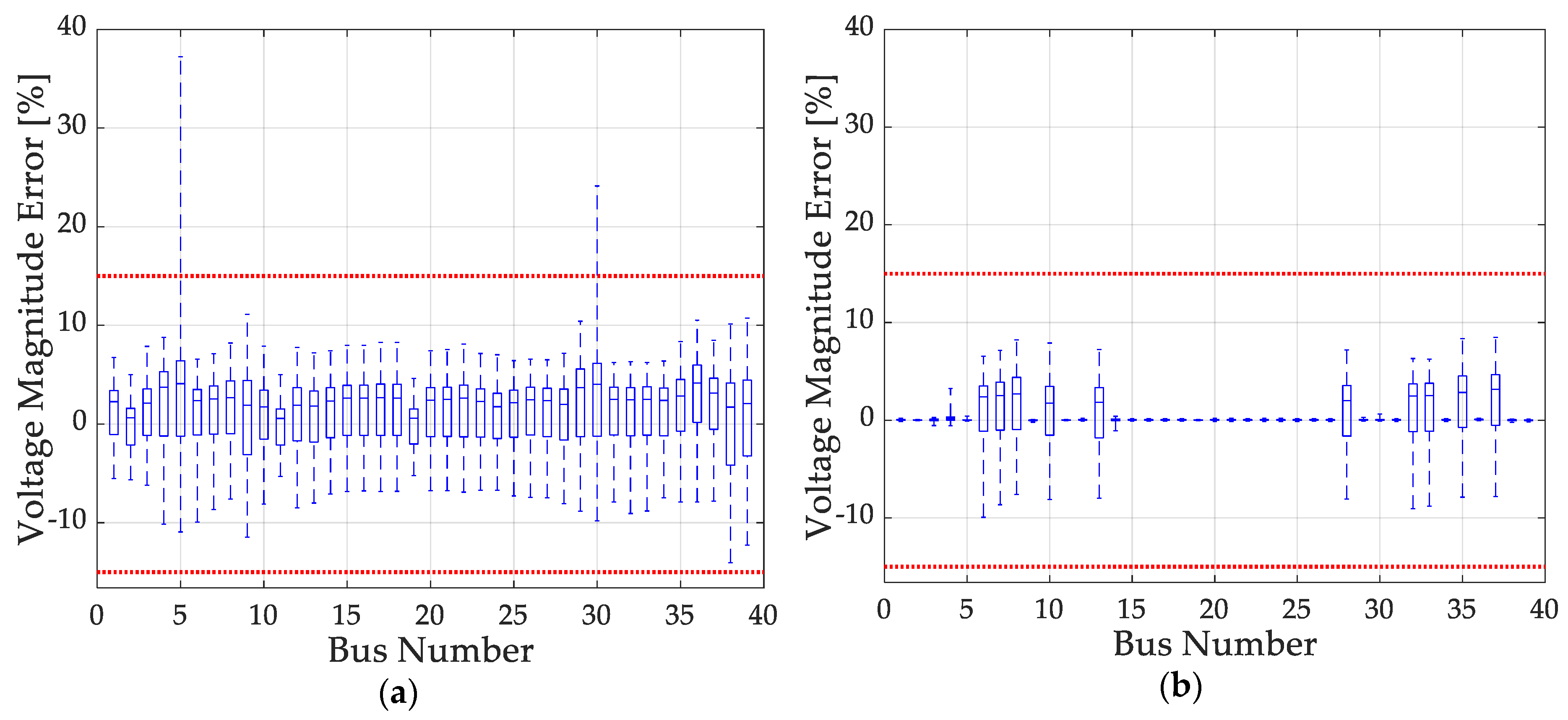
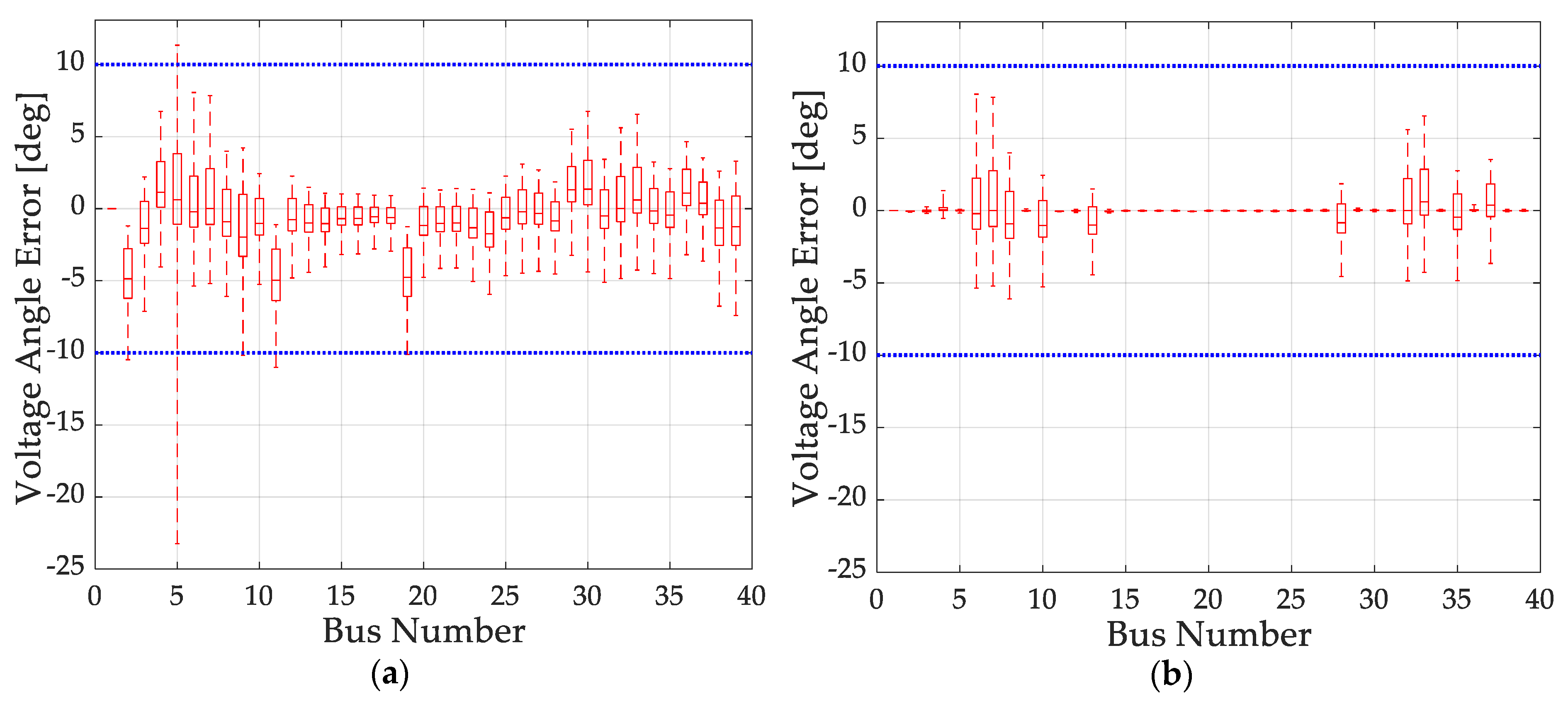
2.2. Hybrid State Estimation with Measurment Uncertainty Propagation of Phasor Measurement Unit (PMU) Measurements

As previously mentioned, HSE is carried out by combining the RTU and the PMU. Basically, HSE works in two steps. Firstly, SCADA SE is executed using only data obtained by RTU, and after that, PMU measurement data is overlapped on those estimated states by SCADA SE, and linear SE is executed [16]. Thus, in case of a PMU outage, the power system is still observable as long as SCADA SE survives. The redundancy or reliability of observability in SE are not the topic of this paper, thus they are not considered in the numerical experiment.
The estimated state by SCADA SE is voltage vector, and the PMU measurement value is also voltage vector, whereby both of them become a new measurement vector. Therefore, the relationship between the new measurement vector and the new state vector becomes linear, and the measurement equation becomes linear as follows [16]:
z = H x + ε
where, z’ is the new measurement vector composed of the bus voltage phasor state vector previously obtained by SCADA SE and the bus voltage phasor measurement vector. x is the new voltage phasor state vector, H’ is the new linear Jacobian matrix, and ε’ is the new measurement error vector. The detail of the equation can be represented by the following equation:
[ V R S C A D A V I S C A D A V R P M U d V I P M U d V R P M U p V I P M U p ] = [ H 11 H 12 H 21 H 22 H 31 H 32 H 41 H 42 H 51 H 52 H 61 H 62 ] [ V R V I ] + [ ε V R S C A D A ε V I S C A D A ε V R P M U d ε V I P M U d ε V R P M U p ε V I P M U p ]
where, superscripts SCADA, PMUd, and PMUp indicate the estimated state by SCADA SE, the PMU direct measurement value and the PMU pseudo measurement value, respectively. Subscripts VR, VI, R, and I mean the real and imaginary value of the complex voltage, and the measurement error for real and imaginary voltage, respectively. Direct measurement is the measurement value obtained by PMU directly. Pseudo measurement is the measurement value obtained by calculation using several direct/pseudo measurements already obtained. In the pseudo measurements, the measurement error can be bigger than the direct measurement by measurement uncertainty propagation. The authors have proposed the MOOPP formulation to consider the influence of the uncertainty propagation which occurs in the use of zero injection, the detail of which is explained in our previous paper [19]. Hereby, the measurement equation is linear, and is easily solved by the following equation without any iterations:
G x ^ = H T R 1 [ z H x ]
where, x ^ is the estimated state vector, G′ = HTR−1H′ is the new gain matrix, and R′ = diag{R, RPMUd, RPMUp} is the extended diagonal covariance matrix of measurement error. RPMUd and RPMUp are formed by measurement error variance of direct measurement and pseudo measurement with uncertainty propagation, respectively.
Measurement uncertainty propagation occurs in PMU pseudo measurements, such as obtaining bus voltage phasor adjacent to the PMU direct measurement bus by Ohm’s law, etc. Firstly, the standard uncertainty in the measurement can be expressed as follows [24]:
u ( p ( k ) ) = Δ p ( k ) 3
where, Δp(k) is the maximum uncertainty specified by the meter manufacturer in the measurement p(k). This paper determines the maximum measurement uncertainty of each meter with reference to an article by Valverde et al. [21]. By the classical uncertainty propagation theory [24], uncertainty of pseudo measurement is affected by the set of measurement uncertainty that calculates it. Thus, measurement uncertainty of pseudo measurements is generally given by:
u ( n ) = k = 1 m [ n p ( k ) u ( p ( k ) ) ] 2
where, p is a measurement vector used to compute the pseudo measurements in this case, and u(n) is the standard uncertainty of measurement n. m is the length of vector p.

3. Voltage Stability Index Calculation

In VSI research, there are some different types of voltage stability indices:
  • Sensitivity analysis by Jacobian
  • Bus VSIs
  • Line VSIs
The sensitivity analysis is carried out by a linearized equation representing the relationship between active and reactive power, and voltage angle and magnitude [1]. Bus VSIs evaluate the voltage stability of system buses, normally given by Thevenin’s equivalent circuit [6]. This research focuses on line VSIs for the evaluation method of system voltage stability as they are simple and easy to implement.

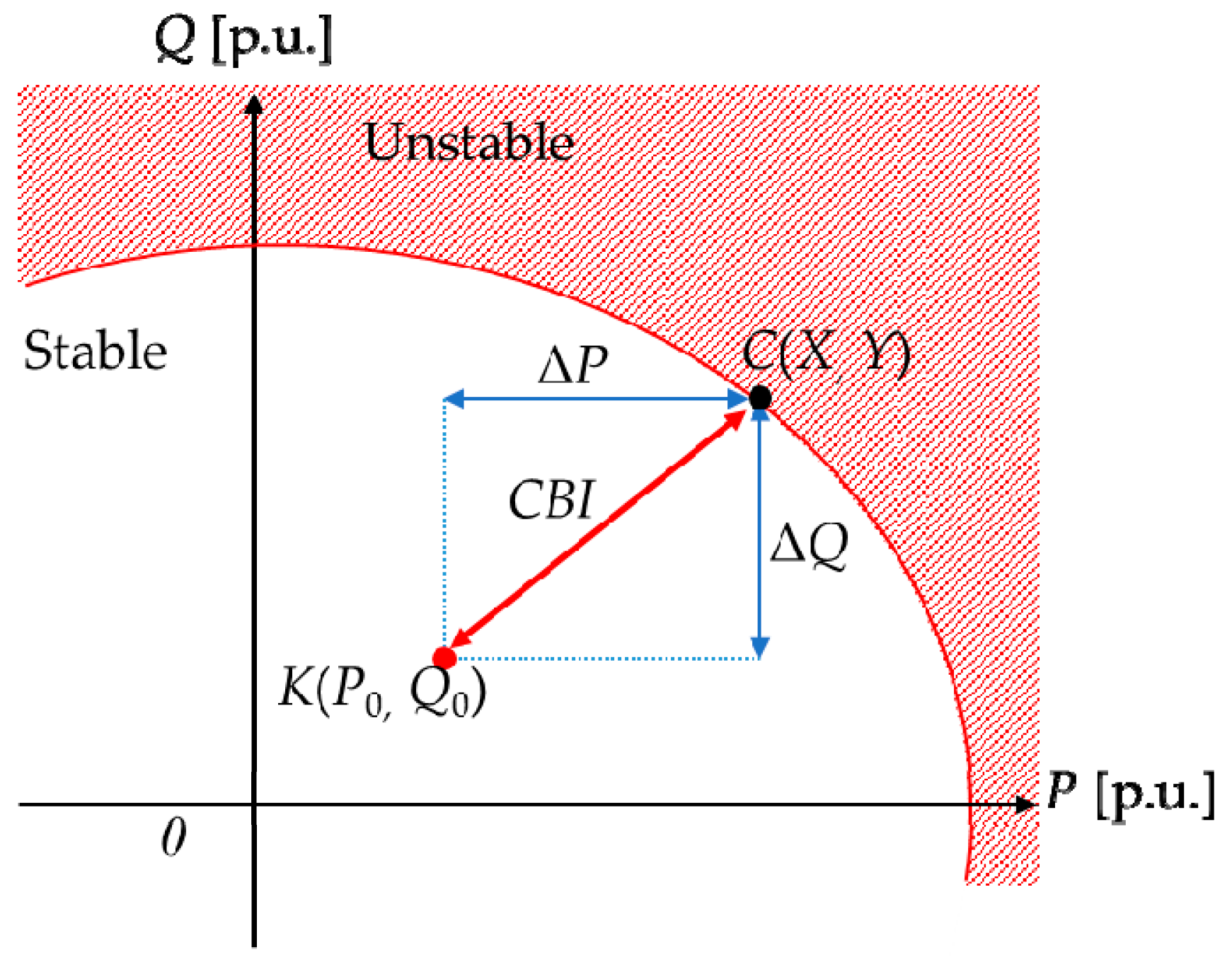
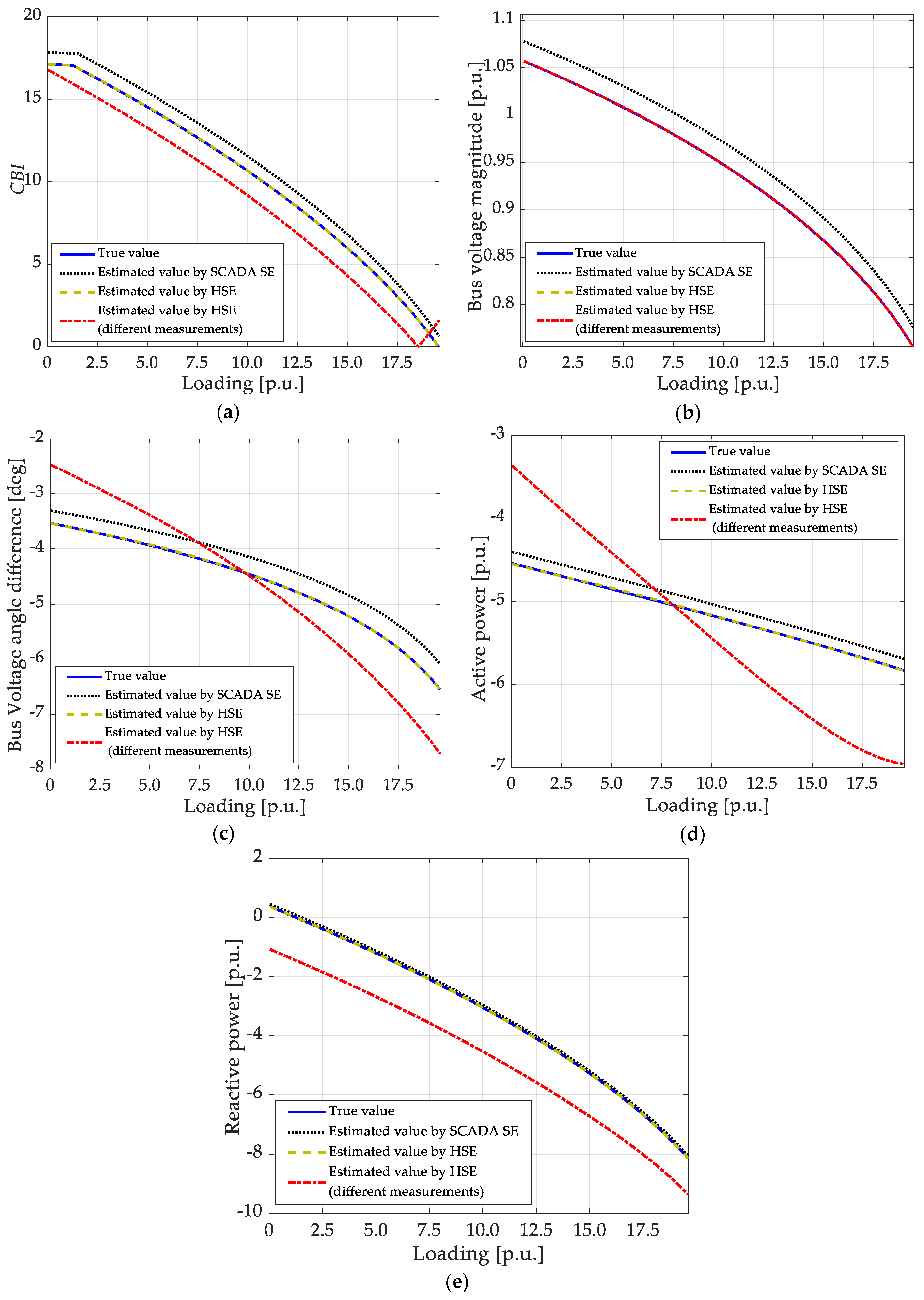
3.1. Critical Boundary Index

CBI was proposed by Furukakoi et al. [20] in 2018. The transmission line model of a 2 bus system is illustrated in Figure 1. Receiving complex power in which the shunt components are ignored for simplification is represented as follows [20]:
P l + j Q l = V l θ l ( V k θ k V l θ l R k l + j X k l ) *
where, Pl and Ql are active and reactive power flow at the receiving end, respectively. Vl and Vk are voltage magnitude at the receiving and sending ends, respectively. θl and θk are voltage angle at the receiving and sending ends, respectively. rkl and xkl are resistance and reactance on line k-l. By separating the real and imaginary parts of (11), the following equation can be derived:
( P l R k l + Q l X k l ) + j ( P l X k l Q l R k l ) = V k V l cos ( θ k θ l ) j V k V l sin ( θ k θ l ) V l 2
By summation of the real and imaginary parts of (12) using sin2θ + cos2θ = 1:
( P l R k l + Q l X k l + V l 2 ) 2 + ( P l X k l Q l R k l ) 2 = V k 2 V l 2
( V l 2 ) 2 + 2 ( P l R k l + Q l X k l V k 2 2 ) V l 2 + ( R k l 2 + X k l 2 ) ( P k l 2 + Q k l 2 ) = 0
Hereby, (14) is a biquadratic equation, V l 2 can be derived as follows:
V l 2 = ( P l R k l + Q l X k l V k 2 2 ) ± ( P l R k l + Q l X k l V k 2 2 ) 2 ( R k l 2 + X k l 2 ) ( P k l 2 + Q k l 2 )
From (15), the voltage stability limit is valid when the part of square root is 0.
To verify the distance between the current operation point and the critical boundary point, Lagrange Multiplier is applied, and (15) can be represented as follows.
C ( X , Y ) = ( P l R k l + Q l X k l V k 2 2 ) 2 ( R k l 2 + X k l 2 ) ( P k l 2 + Q k l 2 ) = 0
The distance between the current operation point K(P0,Q0) and the nearest voltage stability critical boundary point C(X,Y) is a function of f(X,Y). The minimum distance between them is given by:
f 2 = ( X P 0 ) 2 + ( Y Q 0 ) 2
The graphical explanation is shown in Figure 2. The following equations are obtained by using Lagrange multipliers:
F ( X , Y , λ ) = f 2 ( X , Y ) λ C ( X , Y )
F ( X , Y , λ ) = ( X P 0 ) 2 + ( Y Q 0 ) 2 λ ( ( X R k l + Y X k l V k 2 2 ) 2 ( R k l 2 + X k l 2 ) ( X 2 + Y 2 ) )
By applying the partial derivative for X, Y, and λ in the above equation, the following equation can be obtained:
2 X 2 P 0 λ ( 2 ( X R k l + Y X k l V k 2 2 ) R k l 2 ( R k l 2 + X k l 2 ) X ) = 0
2 Y 2 Q 0 λ ( 2 ( X R k l + Y X k l V k 2 2 ) X k l 2 ( R k l 2 + X k l 2 ) Y ) = 0
( X R k l + Y X k l V k 2 2 ) 2 + ( R k l 2 + X k l 2 ) ( X 2 + Y 2 ) = 0
Solving nonlinear Equations (21)–(23), the values of X, Y, and λ are simultaneously obtained. The nearest stable operating point is determined by these values [17]. After obtaining X and Y, the shortest distance between the current operation point and the critical boundary is expressed as follows:
Δ P k l = X P 0
Δ Q k l = Y Q 0
C B I k l = Δ P k l 2 + Δ Q k l 2
The obtained CBIkl is the Critical Boundary Index on the line k-l. CBI approaches from a certain value to 0, which means the voltage stability limit.

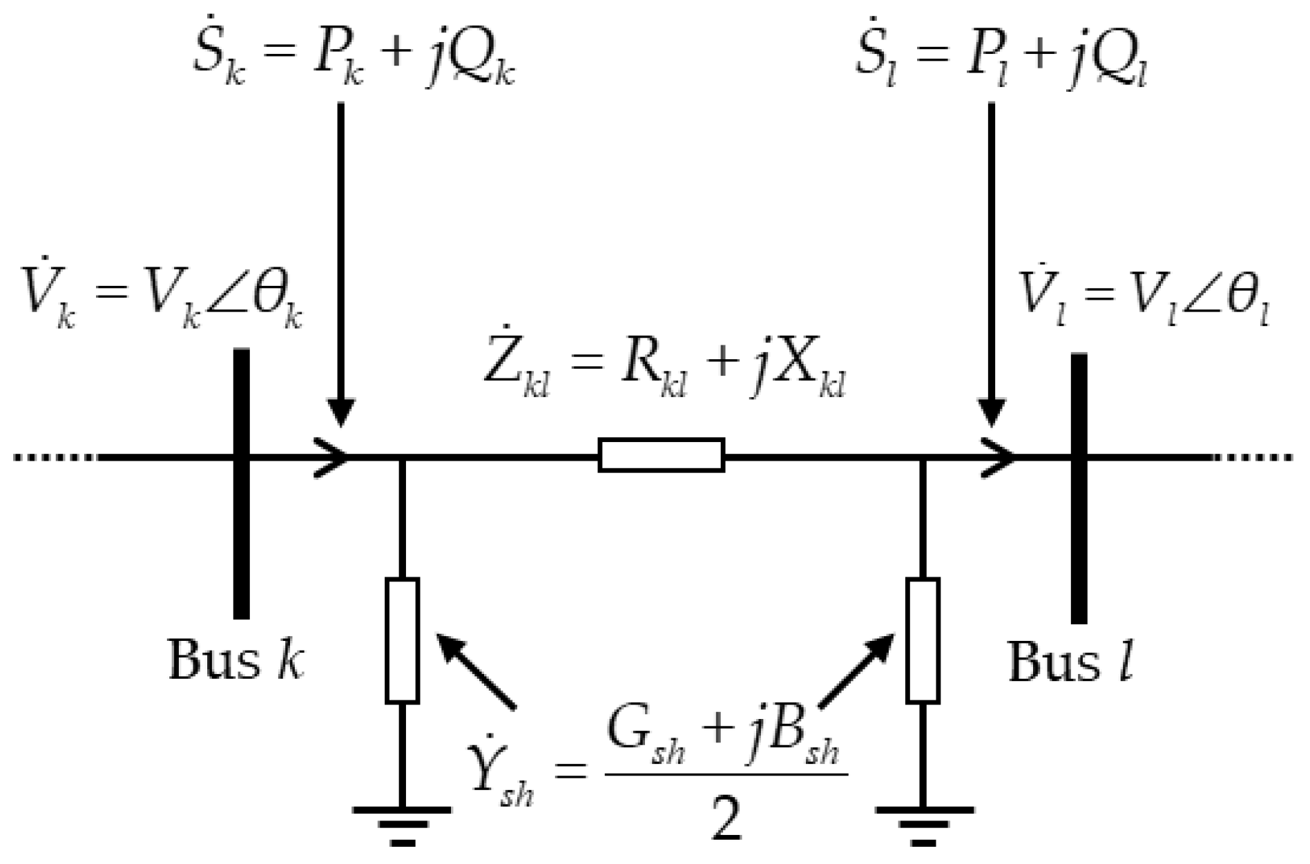
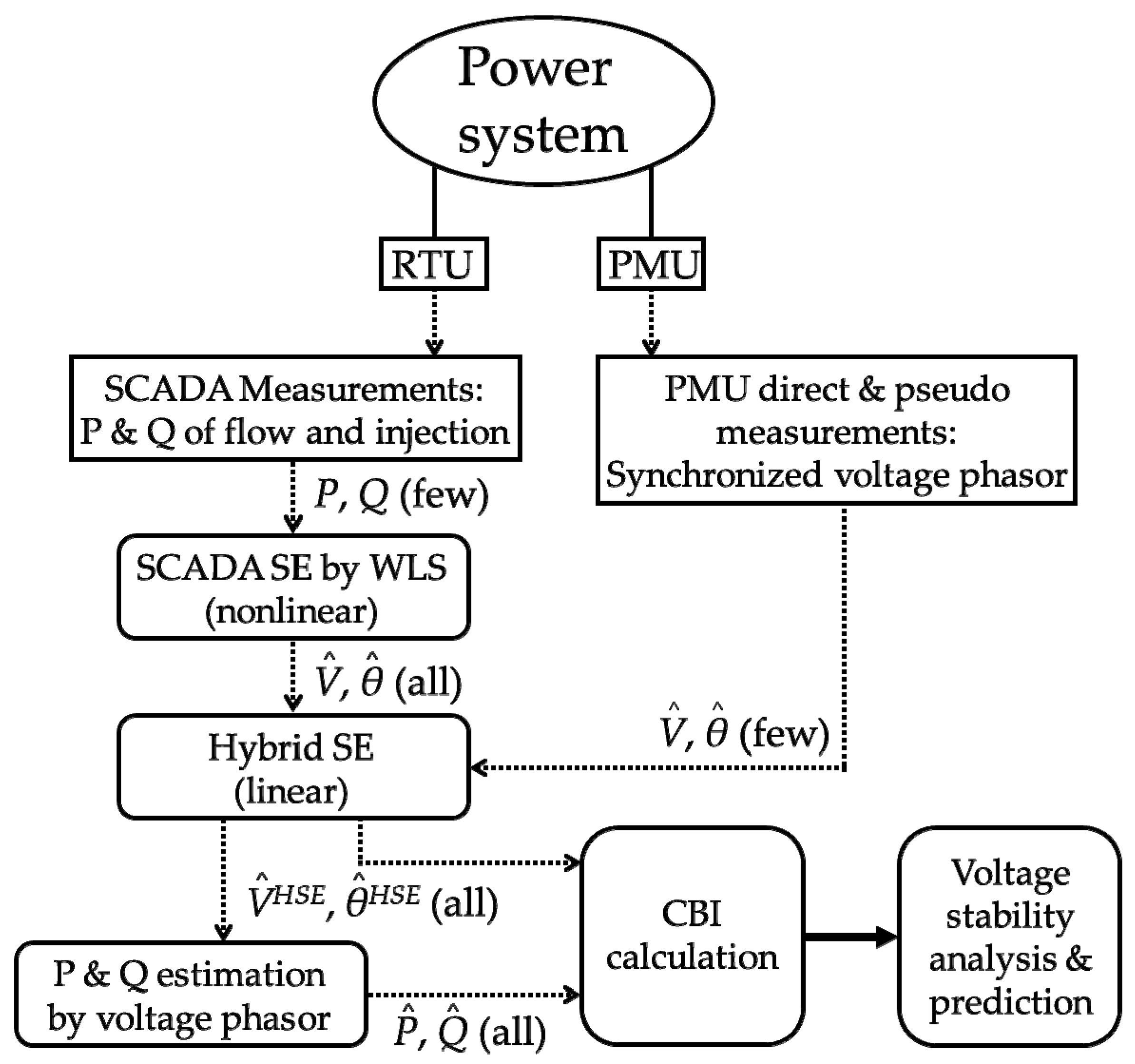
3.2. Active and Reactive Power Estimation by Obtained Bus Voltage Phasor

In order to calculate CBI on the line k-l, the active/reactive power flow needs to be known. Thus, in this paper, estimation of active/reactive power is carried out using estimated voltage phasor as the state vector by HSE. By estimation of the whole system line active/reactive power in appreciation of PMU measurement data, it can treat a case in which there is an insufficient number of RTUs in the power system since the system is observable (voltage phasor at all buses are known), and it means the active/reactive power flow is more accurate. The receiving-end active and reactive power considering the shunt component are calculated as follows:
P l = V l 2 ( G s h + G k l ) + V k V l ( G k l cos ( θ k l ) + B k l sin ( θ k l ) )
Q l = V l 2 ( B s h B k l ) + V k V l ( G k l sin ( θ k l ) + B k l cos ( θ k l ) )
where, G and B indicate conductance and susceptance, respectively. The subscripts sh and kl are the shunt and the line components, respectively. θkl is the voltage phase difference between nodes k and l. The conceptual procedure of CBI estimation using voltage phasor obtained by HSE is depicted in Figure 3.

4. Multi Objective Optimal Phasor Measurement Unit (PMU) Placement

There has been a lot of research on the Optimal PMU Placement (OPP) problem. To make it flexible, MOOPP has been proposed and solved by some researchers, especially using the Pareto approach [25,26,27]. Because of the engineering nature, minimizing the PMU placement cost and the SE error is a trade-off relationship. The Pareto approach is pretty effective for obtaining multiple solutions in trade-off objectives, not to obtain a single solution by the weighting method that may not be able to find the one which the decision maker hopes to know. This section formulates the MOOPP problem and introduces the method to obtain the Pareto optimal solutions.

4.1. Formulation

Because the PMU is still rather expensive, it is impossible to place PMUs at all system buses, the system operator wants to minimize the PMU placement cost. However, in order to improve the voltage security monitoring level by SE, the estimation error of the whole power system needs to be reduced by placing many PMUs on the system. Thus, this confliction can be formulated as a multi-objective optimization problem given by the following objective function and inequality constraints previously represented by the authors [18,19]:
M i n i m i z e   { K V C ,   T V E max }
y y T > 0
( 100 | V i V ^ i | | V i | ) j < E max m a g   ( i = 1 ,   n b ) ( j = 1 ,   n p )
( | θ i θ ^ i | ) j < E max a n g   ( i = 1 ,   n b ) ( j = 1 ,   n p )
where, KVC indicates the total PMU placement cost and TVEmax is the maximum mean value of Total Vector Error (TVE) in all system buses for all SE scenario sets. Both details will be given later. y is the PMU placement decision variable vector given by zeros and ones. If yi as an element of y is 1, a PMU is placed at bus i, otherwise y = 0. Thus, (29) is set to avoid placing none of the PMUs in the system. Vi and θi are voltage magnitude and angle in polar form, respectively. The hat (^) upon them indicates the estimated values whereas those without a hat mean true values E m a x m a g and E m a x a n g are limits of voltage magnitude and angle error, respectively. nb is the number of buses in the power system, np is the considered number of power flow scenarios. As a prior condition, RTUs are already placed at the system redundantly, according to the two-step HSE procedure in Section 2. Hence, the binary decision variable of this MOOPP only deals with PMU voltage/current channel placement.
The authors proposed the novel formulation of MOOPP having considered the PMU current phasor measurement channel selection in the previous paper [18]. It was proven that the current-channel-selectable MOOPP is effective in reducing the redundant current channel and is able to obtain better Pareto optimal solutions compared to the one without considering the current channel placement. Additionally, it is still effective even if the measurement uncertainty propagation is considered [19]. From the authors’ previous articles, the MOOPP strategy in this paper includes both the current channel placement selectivity and measurement uncertainty propagation in HSE. Thus, the PMU cost function KVC is represented by the following equation:
K V C = w v y y T + w c ( D T b ) T b
where, b = [1, …, 1] with the length of nb. D is the decision variable for the current channel selection, in which the element dij is 1 if the current channel is placed at line i-j otherwise 0. Since D is based on the bus connectivity, it is a diagonal matrix. wv and wc are cost weight coefficients for a PMU itself with a voltage measurement channel and a current measurement channel, respectively.
TVE is used to evaluate SE error as the following equation:
T V E max = max 1 j n p { 1 n b i = 1 n b ( V R i , j V ^ R i , j ) 2 + ( V I i , j V ^ I i , j ) 2 }
where, V R i , j and V I i , j are the real and imaginary parts of the true complex voltage at bus i in case of power flow scenario j, respectively. The hat mark upon the variable indicates the estimated value. The content of the summation indicates the Euclidean distance between the true and the estimated value in the rectangular form.
Generally, the objectives KVC and TVEmax are in a trade-off relationship with each other. Thus, in order to improve the objective function value, it is necessary to obtain a solution which has at least no choice but to deteriorate the other one. This solution is called the Pareto optimal solution. The set of Pareto optimal solution is called a Pareto front.

4.2. Optimization Method

For solving the above-mentioned optimization problem (28) under constraints (29–31) by the Pareto approach, this paper employs the Non-dominated Sorting Genetic Algorithm II (NSGA-II) as a multi-objective optimization method. Since the NSGA-II was first devised by Deb et al. in 2002, it has been the most widely used and popular method in the multi-objective optimization [22]. The NSGA-II has reasonable solution search performance by features such as solution selection by congestion distance calculation to maintain the population diversity, non-dominated fast sorting of obtained solutions contributing to Pareto solution accuracy improvement, and the elitism to increase the search speed. In this paper, since comparing the searching performance among optimization methods is not an issue, we used the NSGA-II as the representative method to solve the multi-objective optimization problem.

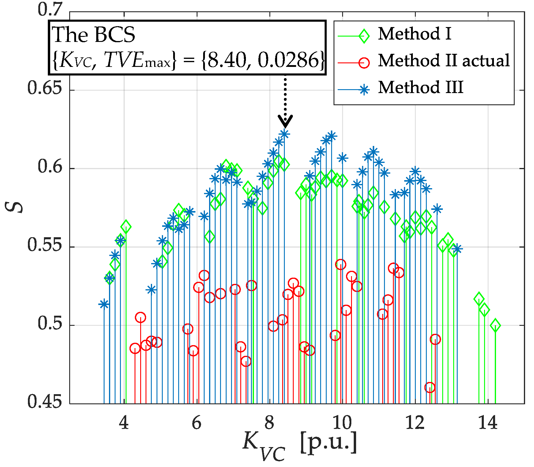
4.3. The Best Compromised Solution Selection

After obtaining the Pareto optimal solutions by the NSGA-II, the decision maker has to select the single solution from the many Pareto optimal solutions: this is highly dependent on the power system operation policy and planning, however. There is a necessity to select the Best Compromised Solution (BCS) as a criterion for the decision maker to determine a single solution [27]. In order to select a solution in terms of the objective satisfaction from the Pareto optimal solutions, satisfaction degree is employed in this paper [27]. The membership function is given by the following equation:
s i = { 1 f i max f i f i max f i min 0 if   f i f i min if   f i min f i f i max if   f i f i max
where, fi is the objective function value of objective i, and f i min and f i max are the minimum and the maximum objective function value of objective i obtained from the Pareto optimal solutions, respectively. The satisfaction degree can be calculated as follows [27]:
S = 1 n o b j i = 1 n o b j s i
where, nobj is the number of objectives, and equal to 2 in the case of this paper, which the first objective is set to KVC, and the second one is set to TVEmax. The BCS is selected with the largest value of S. The meaning of the BCS selected by Equations (34) and (35) is the most balanced solution in those objectives which it can be the criteria solution for the decision of the system operator.

5. Numerical Simulation Results and Discussions

5.1. Configuration

The numerical simulation is given by the following steps tested in modified NE 39-bus. Firstly, multiple Pareto solutions are obtained in MOOPP given by (28–31) using the NSGA-II. After obtaining them, the BCS is selected by (34) and (35) as the most balanced solution in both PMU placement cost and SE accuracy. Next, for the BCS, a statistical box plot is depicted to evaluate how PMU measurement contributes to improve SE accuracy and check the constraint limit. Based PMU placements by the BCS, the huge CBI estimation error caused by voltage phasor estimation in different measurements is confirmed by focusing on a specific line in an active/reactive single loading test. Finally, CBI is calculated for all MCS power flow scenarios in all PMU placements in the Pareto front with or without consideration of discarding voltage phasor by PMU measurement in the mixed measurement case.
The tested power system data, the NSGA-II parameters, and the MOOPP configuration, including meter error of SE and PMU cost, are given by Table 1, Table 2, and Table 3, respectively. The Modified NE-39 was modeled in DigSILENT PowerFactory 2018. SCADA SE, HSE, and NSGA-II were implemented in Matlab R2018a. In Table 3, the PMU cost weight coefficients are set in accordance with costs detailed in an article by Ghamsari–Yazdel and Esmaili [28]. A PMU itself and a voltage measurement channel cost about USD 20,000, the cost of a current measurement channel is about USD 3,000, according to the article. Thus, these weight coefficients are converted as per unit values in Table 3. For Table 3, the RTU and PMU measurement error is assumed as: the maximum measurement uncertainty is specified by the meter manufactures, the probability distribution of measurement uncertainty is assumed as Gaussian distribution, and the measurements are not correlated with each other (independent). The considered power flow scenarios are produced by several loading conditions via MCS [22].

5.2. Pareto Optimal Solutions Obtained by Non-Dominated Sorting Genetic Algorithm II (NSGA-II)

Pareto fronts were obtained by the three different methods below:
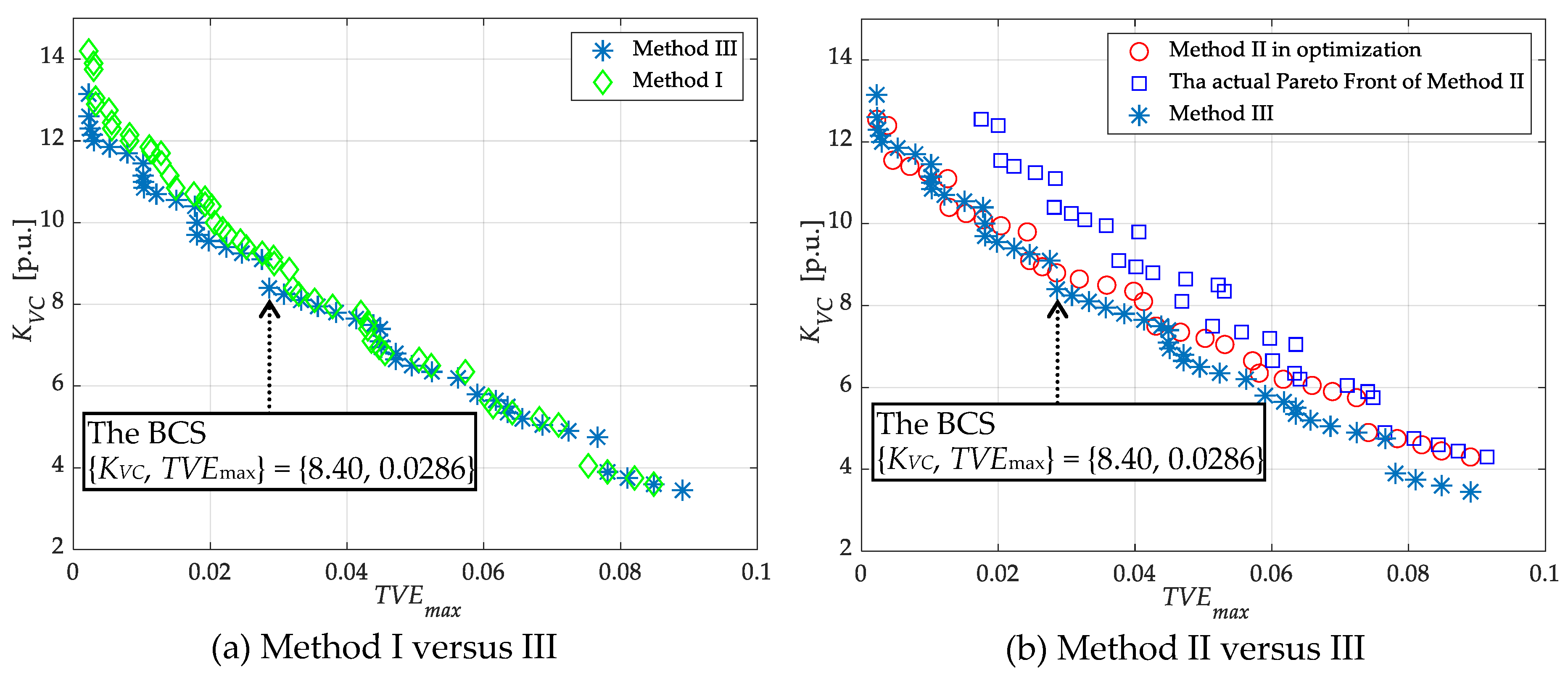
  • Method I: no consideration of the current channel selectivity. The current channel is placed at all lines incident to the PMU placed bus in calculation of KVC. The decision variable is only y.
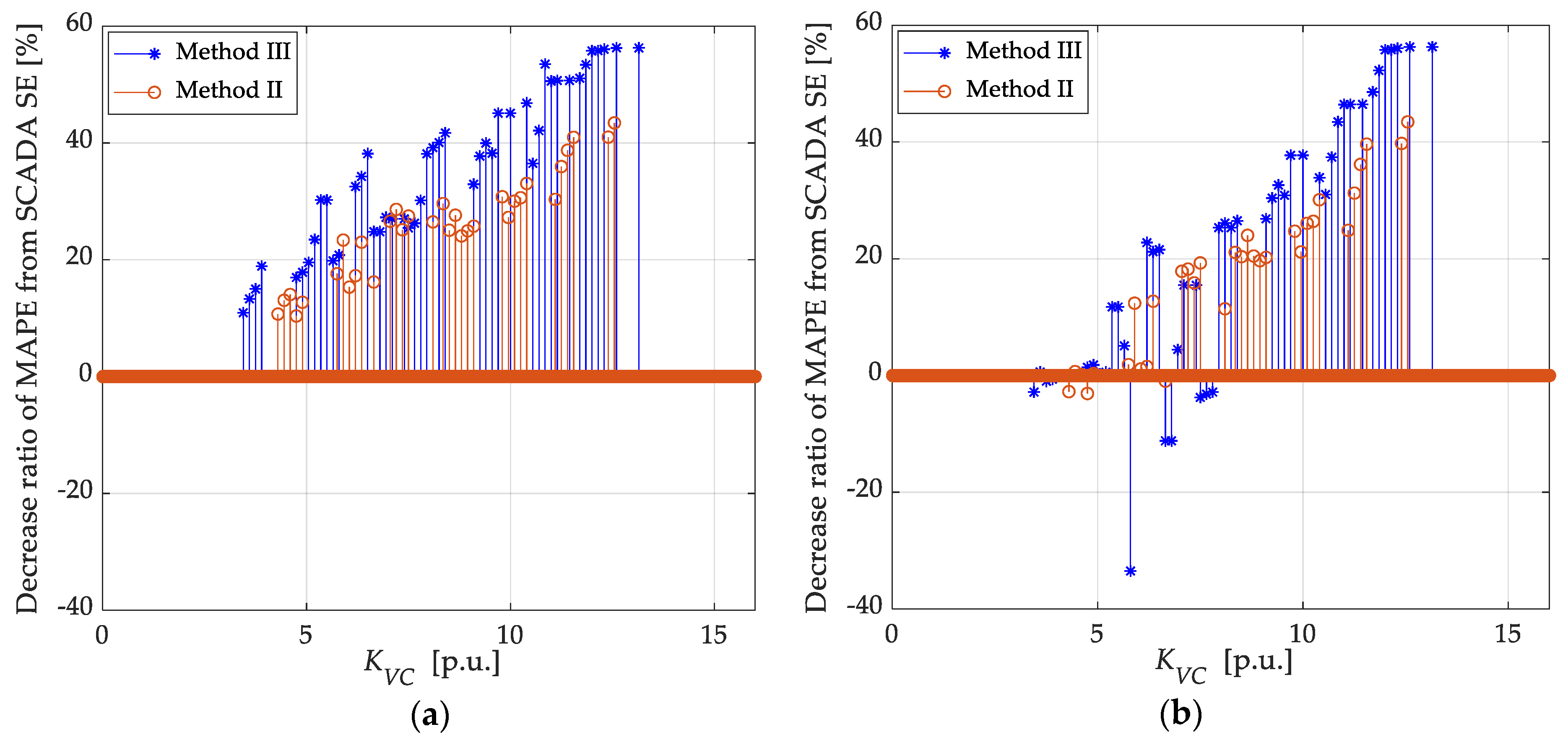
  • Method II: no consideration of measurement uncertainty propagation in PMU pseudo measurement. Measurement uncertainty in HSE is always constant given by Table 3 regardless of the use of pseudo measurement.
  • Method III: with consideration of both the current channel selectivity and measurement uncertainty propagation in PMU pseudo measurements.
Figure 4 shows the obtained Pareto front comparison. The Pareto solutions are distributed from smaller PMU placement cost with worse SE accuracy to larger PMU placement cost with better SE accuracy. Figure 4a shows the Pareto front obtained by Methods I and III. Figure 4b shows the Pareto front obtained by Methods II and III. Since Method I does not include the PMU current channel selection, the PMU placement cost tends to be higher than Method III due to several redundant current channel placements, especially around KVC > 8 (p.u.). Figure 4b shows the comparison of Method II and Method III. In the optimization, some Pareto solutions in Method II are better than Method III, whereas the actual Pareto front in Method II stays apart from Method III. This is caused by ignoring the influence of measurement uncertainty of PMU pseudo measurement especially in case that many PMUs are placed in the power system, meaning many possibilities to use PMU pseudo measurement. Additionally, Method III is numerically proven to be better than the others using the Ratio of Non-dominated Individuals (RNI) [29]. RNI in two methods is calculated by taking the number of non-dominated solutions divided by the sum set of all solutions in the Pareto front of both methods. If RNI > 0.5, the method is better than the other. Table 4 shows the RNI, and therefore, the Pareto front obtained by Method III is quantitatively the best method of the three. Hence, now we have obtained good multiple PMU solutions in terms of SE accuracy and the PMU placement cost.
Figure 5 shows the satisfaction degree S calculated by (33) and (34) in each method. Corresponding to the results in Figure 4, the BCS is obviously determined from Method III. The detailed information of BCS is given in Table 5. The actual PMU placement of the BCS on a single line connection diagram of modified NE 39-bus is shown in Figure 6. As seen in the figure, the PMU current channel is allocated to avoid redundancy. For example, a PMU current phasor channel on line 26–38 is not installed because bus 38 is already observed as a pseudo measurement by the PMU voltage phasor at bus 39 and the current phasor on line 39–38. This sort of channel number reduction cannot be realized by Method I.
Figure 7 and Figure 8 show boxplots of the state SE for all MCS power flow scenarios in SCADA SE, HSE by Placement 1 and 2. The dashed lines are estimation error limit confined in the optimization. In Figure 8 and Figure 9, by placing some PMUs, the estimation error stays within the fixed ranges by improvement of estimation error in some buses.

5.3. CBI Estimation Using Bus Voltage Phasor Obtained by the Hybrid State Estimation (HSE) Based on the PMU Placement

Based on the PMU placement in the BCS chosen from the different Pareto front obtained by NSGA-II multi-objective optimization, CBI as the voltage stability index is calculated by HSE. In this paper, active and reactive loading test in a single load bus was carried out to test the CBI calculation with load increment with a 0.05 p.u. interval. To show an example, CBI estimation and several associated quantities in case of loading at bus 38 are shown in Figure 9a–e. Figure 9a shows the estimation result of the CBI. At the maximum loading point, the CBI finally reaches to almost 0, signifying being on the limit of the voltage stability. In the estimation of CBI, the estimated value by HSE is extremely close to the true value. However, there is a certain deviation in SCADA SE from the true value due to the accuracy of active and reactive power estimation (Figure 9d,e) caused by big errors of the bus voltage phasor estimation (Figure 9c). This result means that SCADA SE which only uses RTU has a risk of misdetection of the voltage instability, possibly triggering a huge blackout. Hence, the system operator is forced to execute a security control action earlier than the actual alarm, which eventually causes more expensive system operational costs.
In Figure 9, another case based on the assumption that the estimated voltage phasor at bus 39 is replaced by a value estimated by SCADA SE (RTU) is shown by the red dashed-dotted line. Since voltage phasors at both buses 35 and 36 were estimated through HSE based on PMU measurements in the previous case, CBI is accurately estimated by HSE. A huge estimation error may occur when voltage phasors at either end are estimated by different measurements. The HSE is characterized by mixed measurements composed of PMUs and RTUs, and this can cause different order values to be subtracted. As seen in Figure 9, CBI estimation by HSE is inaccurate in case of subtraction of the voltage phasor at both ends of a line estimated by mixed measurements and is in fact worse than estimation by SCADA SE while the loading condition gets severe. Voltage phase angle difference is the reason why this huge deviation is created by HSE with voltage phasor at both ends through different estimators.
The voltage phasor at bus 38 is estimated by the PMU measurement, so the estimation error of the voltage phasor at the bus is quite small, as seen in Figure 9. However, if the adjacent bus 39 is assumed not to be estimated by the PMU measurement, then the estimation error is bigger, as seen in Figure 9. This results in the huge error of the voltage phase angle difference because the angle difference is calculated by the subtraction of both voltage phase angle of two buses, which have a different order of error. As seen in Figure 9c, the estimation value of the voltage angle difference between buses 36 and 38 has a certain deviation which results in the estimation error of active power and reactive power computed by (26) and (27) from the true value. Therefore, if a bus is estimated by the PMU measurement and the adjacent bus is not, HSE may not work as well as in the case where both buses are estimated by the PMU measurement. Therefore, the use of estimated voltage phase angle by HSE is not advised if both buses are not measured by PMU.
In order to validate that the discarding state variable estimated by the PMU measurement in case of mixed measurement at two buses of a line, the Mean Absolute Percentage Error (MAPE) of CBI is calculated in cases of SCADA SE and HSE based on all Pareto solutions from Methods II and III. MAPE for CBI estimation is calculated as follows:
M A P E = 1 n l l = 1 n l ( 100 n k = 1 n | C B I ^ k C B I k C B I k | ) l
where, n is the total number of samples (MCS scenarios), and nl is the number of lines. The hat mark upon the CBI indicates the estimated value, whereas no mark upon the CBI indicates the true value. Figure 10 shows how PMU placement improves the CBI estimation accuracy over SCADA SE alone. In Figure 10a, the CBI is calculated based on discarding the voltage phasor estimated by PMU measurement in case of mixed measurement at both ends of a line. Obviously, Method II is deteriorated from Method III because the voltage phasor estimation accuracy is potentially worse than Method III, as seen in Figure 4b. In Figure 10b, the CBI is calculated regardless of the existence of mixed measurements in buses. There is the same tendency with Figure 10b at the region of the many PMUs for a decreased rate of MAPE from SCADA SE. However, it intensively drops in accordance with the decreasing of the PMU placement cost. It even deteriorates to a negative decrease rate, indicating that the MAPE is averagely worse than SCADA SE on its own. This deterioration is clearly caused by a huge error in the mixed measurements in HSE, ignoring subtraction of the voltage phasor estimated by different types of measurements, confirmed by the instance in Figure 9.

6. Conclusions

In this work, CBI as a voltage stability index was evaluated by power system state estimation in both HSE and SCADA SE. HSE includes PMUs and RTUs, the optimal PMU placement was obtained by solving the multi-objective optimal PMU placement problem which minimizes the total PMU placement cost and the state estimation error using the NSGA-II. As a result of numerical simulation in the modified NE 39-bus, the PMU current channel allocation and measurement uncertainty propagation in PMU pseudo measurement were considered in order to obtain a better Pareto front. From the Pareto front, a single solution as the BCS, which is the most balanced solution between the PMU placement cost and the state estimation error, was chosen by membership-function-based satisfaction degree. CBI was computed based on the estimated bus voltage phasor as the result of HSE and the computed receiving-end active and reactive power, compared with SCADA SE. Due to the bigger error of the voltage phasor, CBI estimation in SCADA SE is not accurate which may cause the misdetection or false alarm of voltage instability resulting in costly system operation, whereas CBI estimation by HSE is more accurate. However, the mixed measurement case causes the huge estimation error in HSE. This issue can be overcome by discarding a voltage phasor estimated by PMU measurements in such an instance. In summary, this paper hopes to be of value to the system operator when determining PMU placement strategy in the planning stage, and also suggests the way of PMU measurement usage in HSE for voltage stability monitoring using CBI in the operation stage.

Author Contributions

This research was conducted by a collaborative effort among the authors. Y.M. proposed and formulated the novel multi objective optimal PMU placement problem, implemented the HSE and SCADA SE programs to estimate CBI and wrote the paper. M.W. provided the theoretical knowledge in PMU, optimization and voltage stability and reviewed the paper. N.I.A.W. provided detail knowledge on VSI and reviewed the paper. M.L.O. provided knowledge in computational intelligence especially in optimization and reviewed the paper.

Funding

This research received no external funding.

Acknowledgments

This research was supported by the Power System Control Laboratory (WATANABE Lab.), Kyushu Institute of Technology, Japan. The authors are grateful for the feedback of anonymous reviewers and the editors of the journal, their innovative ideas and suggestions helped us a lot in improving the quality of this article.

Conflicts of Interest

The authors declare no conflict of interest.

References

  1. Ajjarapu, V. Chapter 1 Introduction, Chapter 4 Sensitivity Analysis for Voltage Stability. In Computational Technique for Voltage Stability Assessment and Control, 1st ed.; Pai, M.A., Stankovic, A., Eds.; Springer: New York, NY, USA, 2006. [Google Scholar]
  2. NERC. 1996 System Disturbances: Review of Selected Electric System Disturbances in North America. Available online: https://www.nerc.com/pa/rrm/ea/SystemDisturbanceReportDL/1996SystemDisturbance.pdf (accessed on 13 March 2019).
  3. Vargas, L.S.; Quintana, V.H.; Miranda, D.R. Voltage collapse scenario in the Chilean interconnected system. IEEE Trans. Power Syst. 1999, 14, 1415–1421. [Google Scholar] [CrossRef]
  4. Vournas, C. Technical Summary of the Athens and Southern Greece Blackout of July 12, 2004; National Technical University of Athens: Athens, Greece, 2004. [Google Scholar]
  5. Liu, S.; Deng, H.; Guo, S. Analyses and discussions of the blackout in Indian power grid. Energy Sci. Technol. 2013, 6, 61–66. [Google Scholar]
  6. Modarresi, J.; Gholipour, E.; Khodabakhshian, A. A comprehensive review of the voltage stability indices. Renew. Sustain. Energy Rev. 2016, 63, 1–12. [Google Scholar] [CrossRef]
  7. Makasa, K.J.; Venayagamoorthy, G.K. On-line voltage stability load index estimation based on PMU measurements. In Proceedings of the 2011 IEEE Power and Energy Society General Meeting, Detroit, MI, USA, 24–28 July 2011. [Google Scholar]
  8. Chouhan, D.; Jaiswal, V. A literature review on optimal placement of PMU and voltage stability. Indian J. Sci. Technol. 2016, 9, 1–7. [Google Scholar] [CrossRef]
  9. Phadke, A.G.; Thorp, J.S.; Adamiak, M.G. A new measurement technique for tracking voltage phasors, local system frequency, and rate of change of frequency. IEEE Trans. Power Appar. Syst. 1983, 102, 1025–1038. [Google Scholar] [CrossRef]
  10. Phadke, A.G.; Thorp, J.S. Chapter 7 State estimation, Chapter 8 Control with phasor feedback, Chapter 9 Protection systems with phasor inputs. In Synchronized Phasor Measurements and Their Applications, 1st ed.; Pai, M.A., Stankovic, A., Eds.; Springer: New York, NY, USA, 2008. [Google Scholar]
  11. Esmaili, M. Inclusive multi-objective PMU placement in power systems considering conventional measurements and contingencies. Int. Trans. Electr. Energy Syst. 2016, 26, 609–626. [Google Scholar] [CrossRef]
  12. Tran, V.; Zhang, H.; Nguyen, V. Optimal Placement of Phasor measurement unit for observation reliability enhancement. J. Electer. Eng. Technol. 2017, 12, 1921–1931. [Google Scholar] [CrossRef]
  13. Parimalam, L.; Rajeswari, R. Achieving effective power system observability in optimal PMUs placement using GA-EHBSA. Circuits Syst. 2016, 7, 2002–2013. [Google Scholar] [CrossRef]
  14. Abiri, E.; Rashidi, F.; Niknam, T. An optimal PMU placement method for power system observability under various contingencies. Int. Trans. Electr. Energy Syst. 2015, 25, 589–606. [Google Scholar] [CrossRef]
  15. Baldwin, T.L.; Mili, L.; Boisen, M.B., Jr. Power system observability with minimal phasor measurement placement. IEEE Trans. Power Syst. 1993, 8, 705–715. [Google Scholar] [CrossRef]
  16. Jerin, J.; Bindu, S. Hybrid state estimation including PMU measurements. In Proceedings of the International Conference on Control, Communication & Computing, Trivandrum, India, 19–21 November 2015. [Google Scholar]
  17. Tang, J.; Liu, J.; Ponci, F.; Monti, A. Adaptive load shedding based on combined frequency and voltage stability assessment using synchrophasor measurements. IEEE Trans. Power Syst. 2013, 28, 2035–2047. [Google Scholar] [CrossRef]
  18. Matsukawa, Y.; Watanabe, M.; Mitani, Y.; Othman, M.L. Multi objective PMU placement optimization considering the placement cost including the current channel allocation and state estimation accuracy. IEEJ Trans. Power Energy 2019, 139, 84–90. [Google Scholar] [CrossRef]
  19. Matsukawa, Y.; Watanabe, M.; Mitani, Y.; Othman, M.L. Influence of measurement uncertainty propagation in current-channel-selectable multi objective optimal phasor measurement unit placement problem. In Proceedings of the IEEE Power and Energy Society Generation, Transmission and Distribution Grand International Conference and Exposition Asia 2019, Bangkok, Thailand, 19–23 March 2019. [Google Scholar]
  20. Furukakoi, M.; Adewuyi, O.B.; Danish, M.S.S.; Howlader, A.M.; Senjyu, T.; Funabashi, T. Critical Boundary Index (CBI) based on active and reactive power deviations. Int. J. Electr. Power Energy Syst. 2018, 100, 50–57. [Google Scholar] [CrossRef]
  21. Valverde, G.; Chakrabarti, S.; Kyriakudes, E.; Terzija, V. A constrained formulation for hybrid state estimation. IEEE Trans. Power Syst. 2011, 26, 1102–1109. [Google Scholar] [CrossRef]
  22. Deb, K.; Paratab, S.; Agarwal, S.; Meyarivan, T. A fast end elitist multiobjective genetic algorithm: NSGA-II. IEEE Trans. Evol. Comput. 2002, 6, 182–197. [Google Scholar] [CrossRef]
  23. Rakpenthai, C.; Uatrongjit, S. A new hybrid state estimation based on pseudo-voltage measurements. IEEJ Trans. Electr. Electron. Eng. 2015, 10, S19–S27. [Google Scholar] [CrossRef]
  24. ISO-IEC-OMIL-BIPM. Guide to the Expression of Uncertainty in Measurement; JCGM: Sèvres, France, 1992. [Google Scholar]
  25. Milosevic, B.; Begovic, M. Nondominated sorting genetic algorithm for optimal phasor measurement placement. IEEE Trans. Power Syst. 2003, 18, 69–75. [Google Scholar] [CrossRef]
  26. Jamuna, K.; Swarup, K.S. Multi-objective biogeography based optimization for optimal PMU placement. Appl. Soft Comput. 2012, 12, 1503–1510. [Google Scholar] [CrossRef]
  27. Peng, C.; Sun, H.; Guo, J. Multi-objective optimal PMU placement using a non-dominated sorting differential evolution algorithm. Int. J. Electr. Power Energy Syst. 2010, 32, 886–892. [Google Scholar] [CrossRef]
  28. Ghamsari-Yazdel, M.; Esmaili, M. Reliability-based probabilistic optimal joint placement of PMUs and flow measurements. Int. J. Electr. Power Energy Syst. 2016, 78, 857–863. [Google Scholar] [CrossRef]
  29. Knowles, J.D.; Corne, D.W. Approximating the nondominated front using the Pareto archived evolution strategy. Evol. Comput. 2000, 8, 149–172. [Google Scholar] [CrossRef] [PubMed]
Figure 1. Transmission line model.
Energies 12 02688 g001
Figure 2. Critical boundary of the voltage stability in P-Q characteristics.
Energies 12 02688 g002
Figure 3. The Critical Boundary Index (CBI) estimation flow chart.
Energies 12 02688 g003
Figure 4. Obtained Pareto fronts in each method.
Energies 12 02688 g004
Figure 5. Satisfaction degree in each method.
Energies 12 02688 g005
Figure 6. The actual PMU placement of the BCS in modified NE 39-bus.
Energies 12 02688 g006
Figure 7. Statistical box plot of voltage magnitude estimation error in the BCS. (a) SCADA SE, (b) HSE.
Energies 12 02688 g007
Figure 8. Statistical box plot of voltage angle estimation error in the BCS. (a) SCADA SE, (b) HSE.
Energies 12 02688 g008
Figure 9. CBI in case of bus 38 loading. (a) CBI on line 38–39, (b) Voltage magnitude at bus 38, (c) Voltage angle difference between buses 38 and 39, (d) Active power at receiving end on line 38–39, (e) Reactive power at receiving end on line 38–39.
Energies 12 02688 g009
Figure 10. Decrease ratio of the Mean Absolute Percentage Error (MAPE) from SCADA SE for all Pareto solutions in Methods II and III. (a) Discarding estimated state by PMU, (b) Without discarding estimated state by PMU.
Energies 12 02688 g010
Table 1. Numerical information of the modified New England 39-bus test system (NE 39-bus).
ParameterValue
The number of buses39
The number of lines52
The number of load buses19
The number of the current channel placement candidates104
The length of decision variable in MOOPP143
Table 2. Non-dominated Sorting Genetic Algorithm II (NSGA-II) parameters.
ParameterValue/Method
The population size70
Crossover rate0.95
Mutation rate0.05
The number of generations1000
The crossover methodUniform crossover
Table 3. Multi Objective OPP (MOOPP), Supervisory Control and Data Acquisition State Estimation (SCADA SE), and Hybrid State Estimation (HSE) parameters.
ClassParameterValue
MOOPP problemA PMU and a voltage channel cost wV [28]1.0 (p.u.)
A current channel cost wC [28]0.15 (p.u.)
Estimation error limit for voltage magnitude 15 (%)
Estimation error limit for voltage angle10 (deg)
The number of power flow scenarios1000
Maximum measurement uncertainty [21]SCADA injection2 (%)
SCADA flow2 (%)
PMU voltage magnitude0.02 (%)
PMU current magnitude0.03 (%)
PMU phase angle0.01 (deg)
Table 4. Ratio of Non-dominated Individuals (RNI) calculation.
Method IMethod II
Method III0.8125:0.18751:0
Table 5. The details of the Best Compromised Solution (BCS).
ClassValue
PMU placement buses2, 5, 16, 23, 26, 39
Current channel placement lines2-11, 2-19, 5-30, 16-1, 16-15, 16-21, 23-22, 23-24, 26-25, 26-27, 26-29, 26-31, 26-34, 39-9, 39-36, 39-38
KVC8.40
TVEmax0.0286

