Forecasting India’s Electricity Demand Using a Range of Probabilistic Methods


Abstract
1. Introduction
2. Literature Review
2.1. Electric Power Research in India
2.2. Overview of Forecasting Methods
2.3. Research Implication
- (1)
- Methods are changeable. In the research process, linear and nonlinear models are used together, including both independent and combined ones. The five prediction results are compared with each other, and each factor is analyzed in detail to make the research results scientific and persuasive.
- (2)
- The paper uses three statistical parameters (MSE, MSPE, MAPE) to analyze the accuracy of forecast data and calculate the error in each model.
- (3)
- Fill in the research gap of previous methods with linear models or nonlinear models, respectively. Comprehensive applications of predictive models have been expanded, which enriches the research and makes it realistic and applicable.
3. Methods
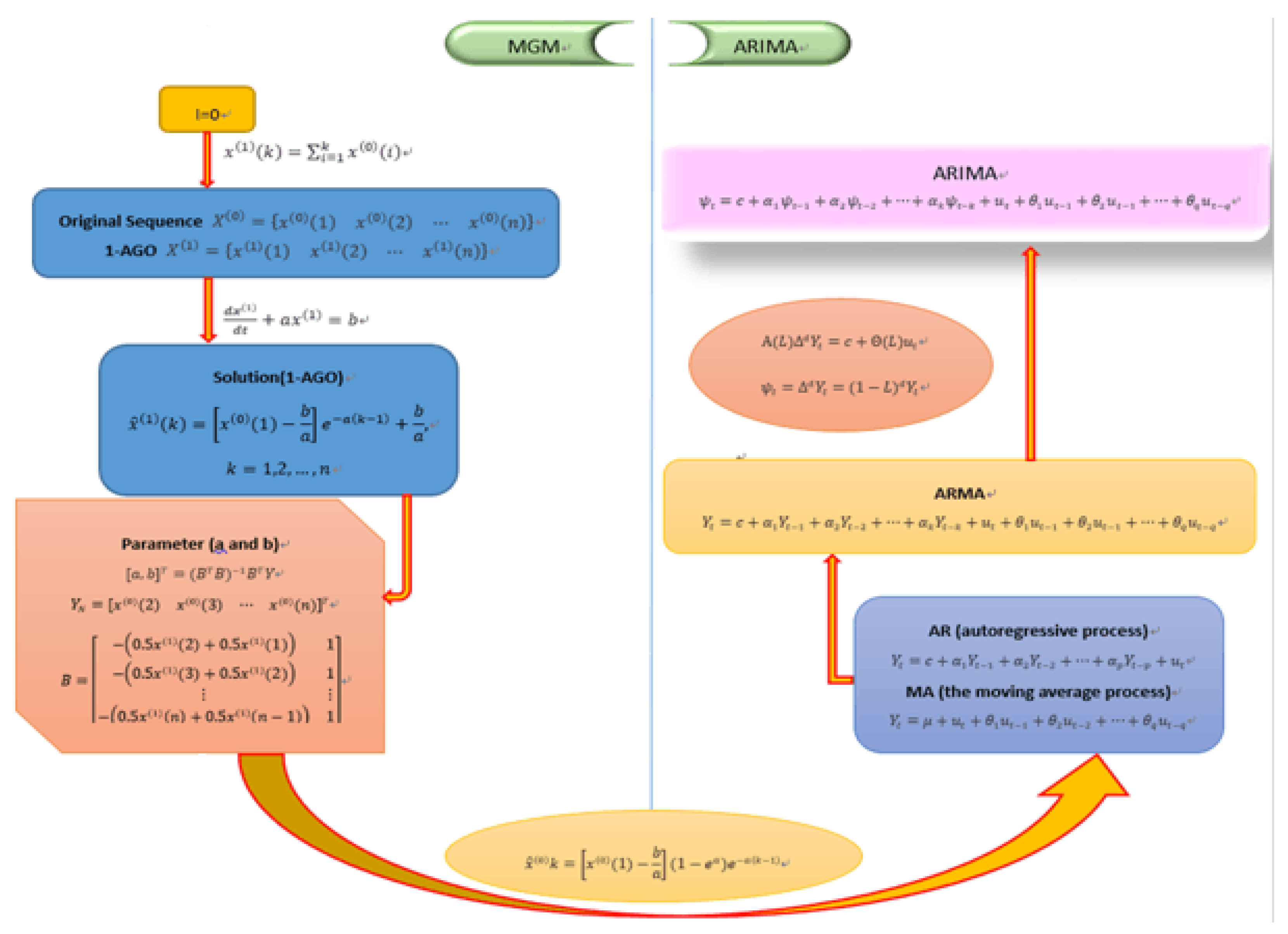
3.1. MGM (1,1) Model
3.2. ARIMA
3.3. MGM-ARIMA
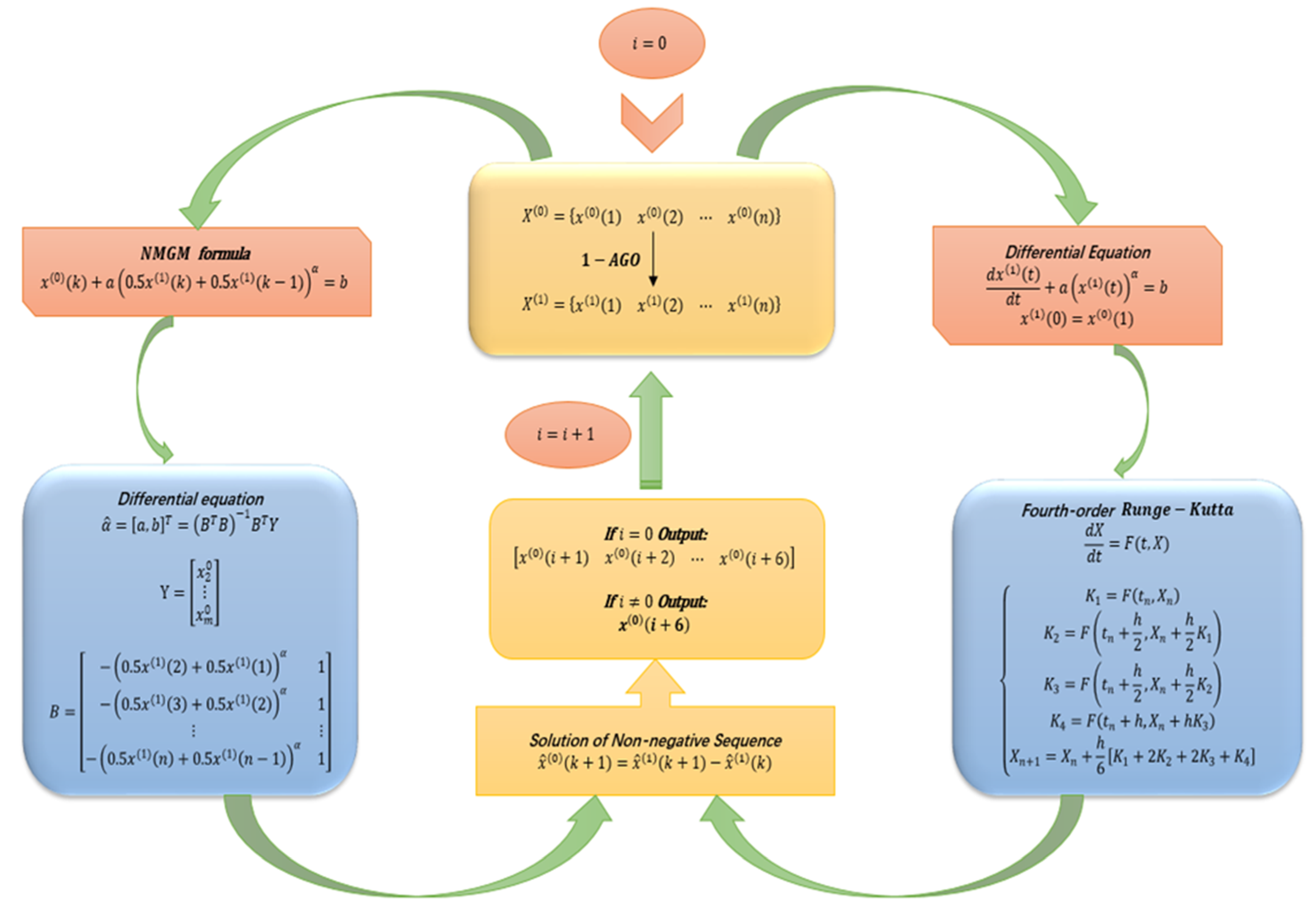
3.4. Nonlinear Metabolic Grey Model
3.5. NMGM-ARIMA.
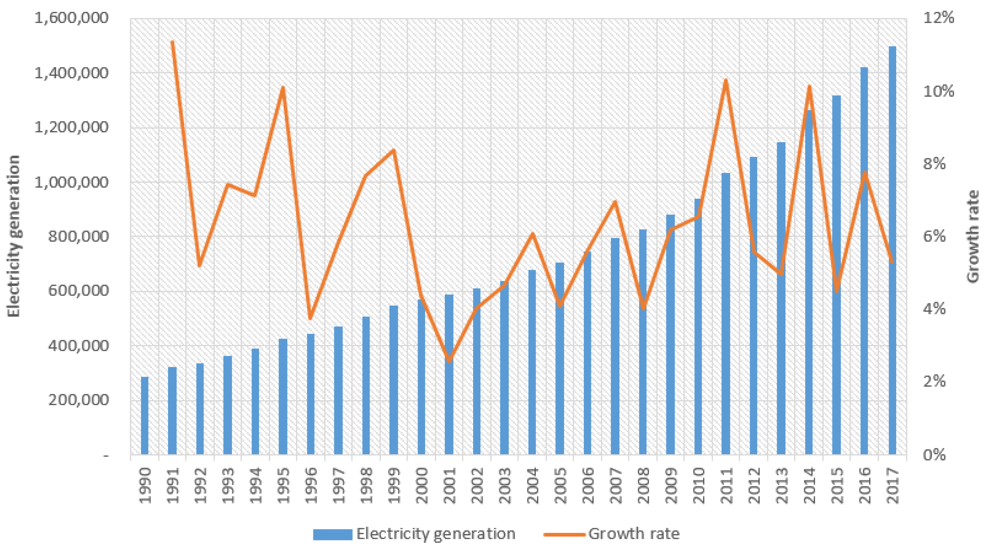
4. Empirical Result
4.1. Fitting Process
4.1.1. MGM (1,1)
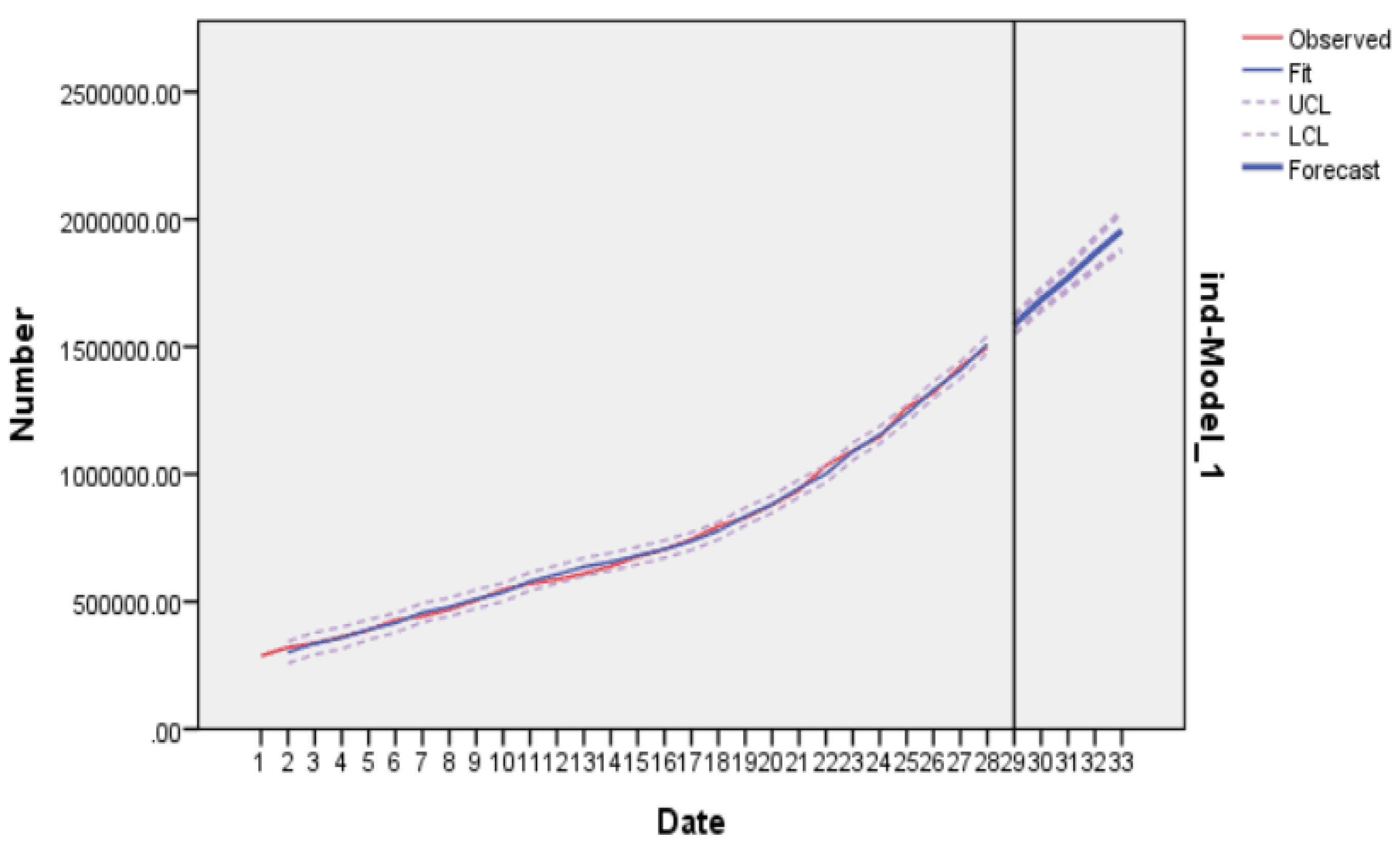
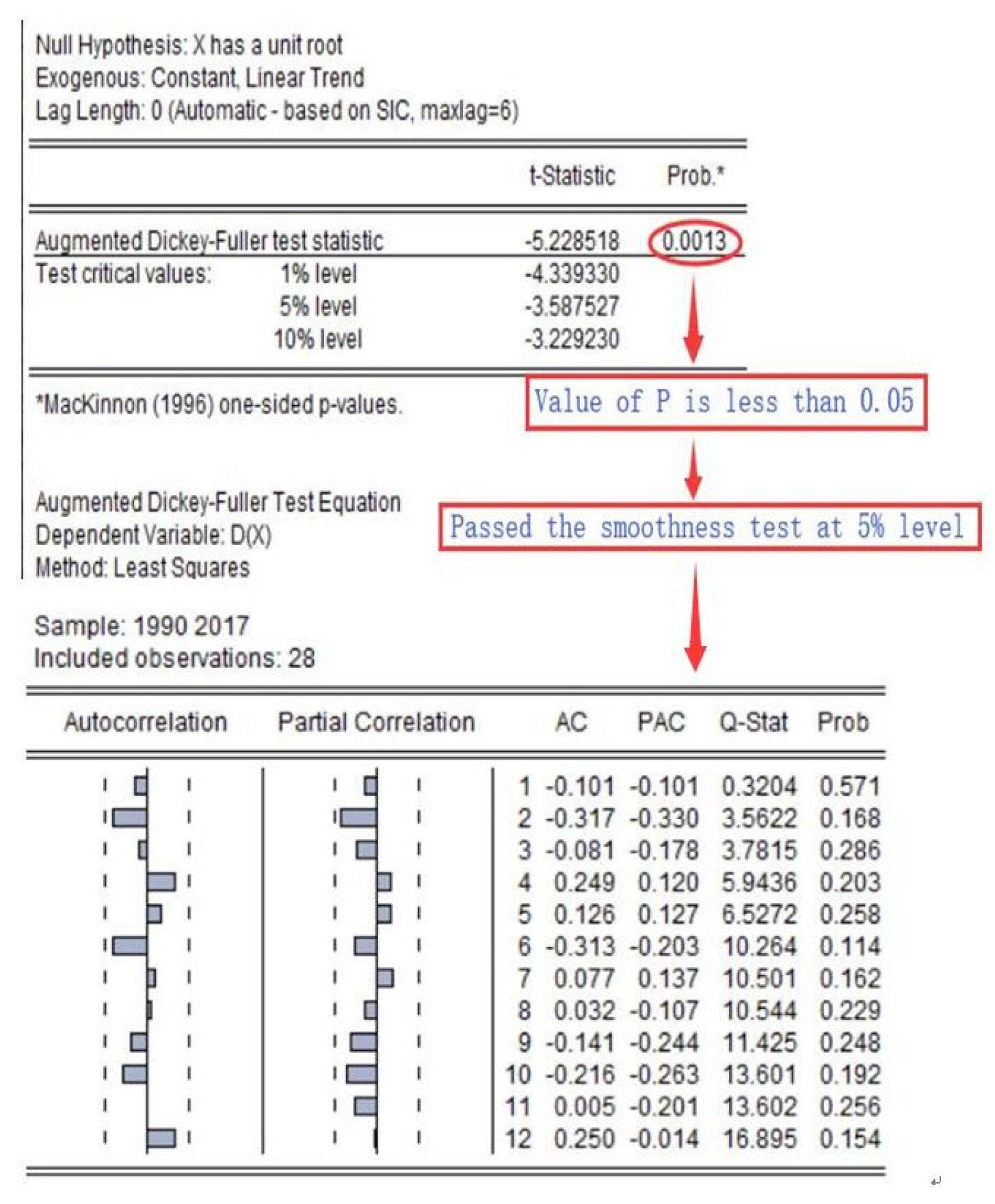
4.1.2. ARIMA
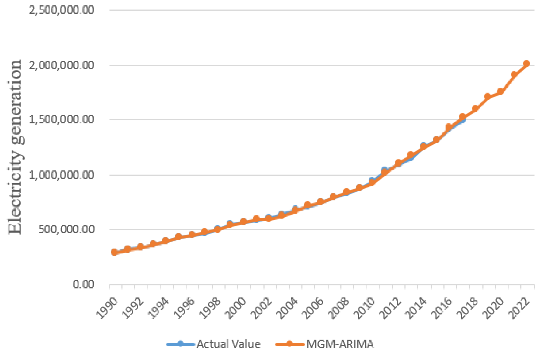
4.1.3. MGM-ARIMA
4.1.4. NMGM
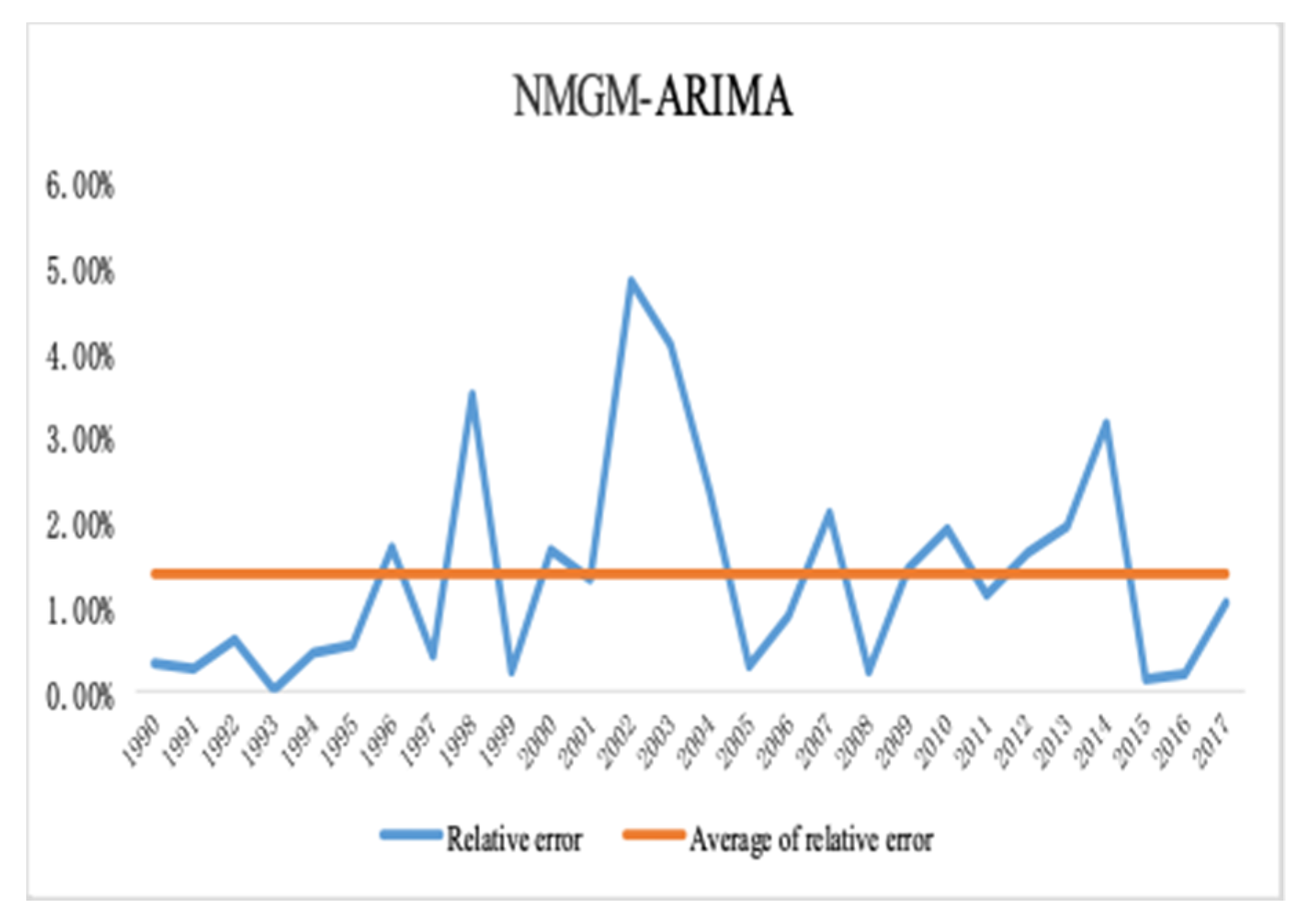
4.1.5. NMGM-ARIMA
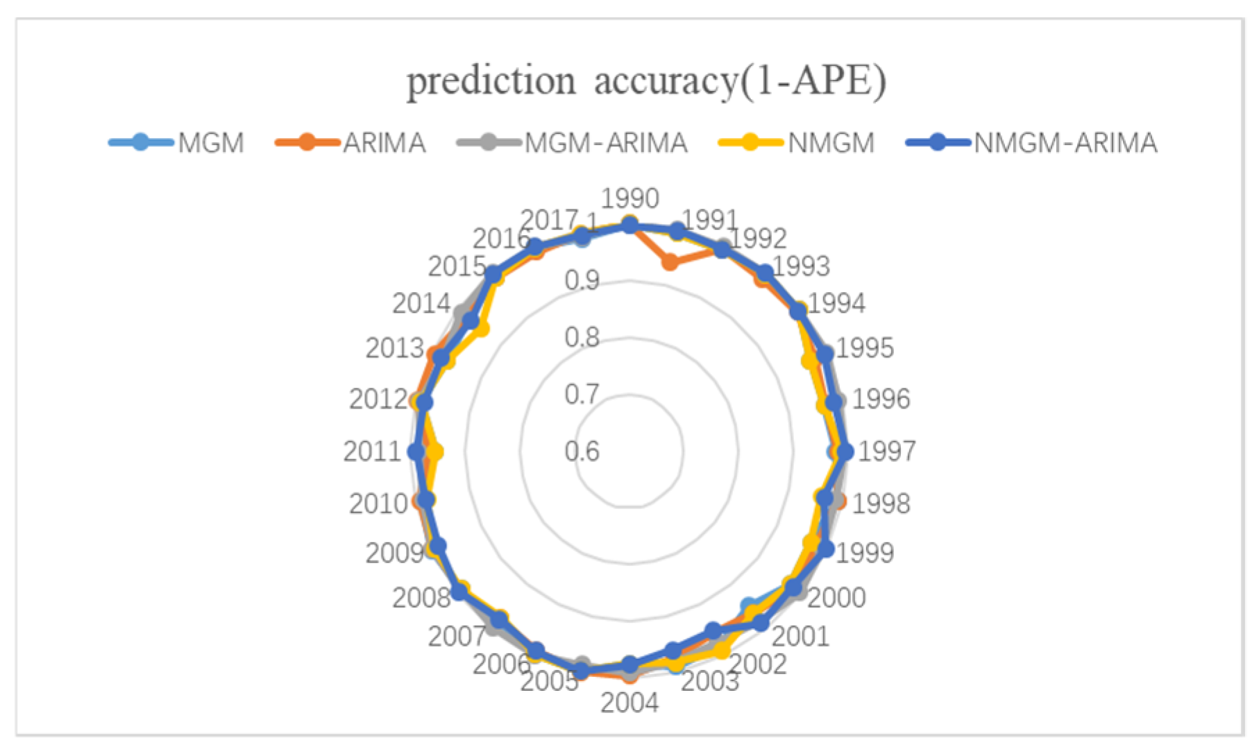
4.2. Optimization Analysis
5. Forecasting Results and Discussion
6. Conclusions
Author Contributions
Funding
Conflicts of Interest
References
- Samir, K.C.; Wurzer, M.; Speringer, M.; Lutz, W. Future population and human capital in heterogeneous India. Proc. Nat. Acad. Sci. USA 2018, 115, 8328–8333. [Google Scholar] [CrossRef]
- Bhanja, S.N.; Mukherjee, A.; Rodell, M. Groundwater Storage Variations in India. In Groundw. South Asia; Mukherjee, A., Ed.; Springer: Singapore, 02 June 2018; pp. 49–59. ISBN 978-981-10-3889-1. [Google Scholar] [CrossRef]
- Shahbaz, M.; Mallick, H.; Mahalik, M.K.; Sadorsky, P. The role of globalization on the recent evolution of energy demand in India: Implications for sustainable development. Energy Econ. 2016, 55, 52–68. [Google Scholar] [CrossRef]
- Xing, W.L.; Chen, Y.C.; Wang, A.J.; Zhou, F.Y.; Yan, Q. India’s future energy demand and its impact on China’s obtaining of overseas resources. Acta. Geosci. Sin. 2017, 38, 45–53. [Google Scholar] [CrossRef]
- Kumar, R.; Jilte, R.; Nikam, K.C.; Ahmadi, M.H. Innovation, Status of carbon capture and storage in India’s coal fired power plants: A critical review. Environ. Tech. Innov. 2018, 13, 94–103. [Google Scholar] [CrossRef]
- Sadath, A.C.; Acharya, R.H. Assessing the extent and intensity of energy poverty using Multidimensional Energy Poverty Index: Empirical evidence from households in India. Energy Policy 2017, 102, 540–550. [Google Scholar] [CrossRef]
- Catia, C.; Reza, M. Household and industrial electricity demand in Europe. Energy Policy 2018, 112, 592–600. [Google Scholar] [CrossRef]
- Saravanan, S.; Kannan, S.; Thangaraj, C. Forecasting India’s electricity demand using Artificial Neural Network. In Proceedings of the IEEE International Conference on Advances in Engineering, Nagapattinam, Tamil Nadu, India, 30–31 March 2012. [Google Scholar]
- Saravanan, S.; Kannan, S.; Thangaraj, C. India’s Electricity Demand forecast using Regression Analysis and Artificial Neural Networks based on principal components. ICTACT J. Soft Comput. 2012, 2, 365–370. [Google Scholar] [CrossRef]
- Mohamed, Z.; Bodger, P. A comparison of Logistic and Harvey models for electricity consumption in New Zealand. Tech. Forecast. Soc. Chang. 2005, 72, 1030–1043. [Google Scholar] [CrossRef]
- Bhowte, Y.W. Forecasting the load of demand and supply of Electricity in India. 2016 International Conference on Computation of Power. In Proceedings of the IEEE Energy Information and Commuincation (ICCPEIC), Chennai, India, 20–21 April 2016. [Google Scholar]
- Singh, D.P.; Gadakh, P.J.; Dhanrao, P.M.; Mohanty, S.; Swain, D.; Swain, D. An Application of NGBM for Forecasting Indian Electricity Power Generation. Adv. Int. Syst. Comput. 2017, 556, 203–214. [Google Scholar] [CrossRef]
- Tisdell, C.C. Technology, Alternate solution to generalized Bernoulli equations via an integrating factor: An exact differential equation approach. Int. J. Math. Educ. Sci. Technol. 2017, 48, 913–918. [Google Scholar] [CrossRef]
- Chen, C.I.; Chen, H.L.; Chen, S.P. Forecasting of foreign exchange rates of Taiwan’s major trading partners by novel nonlinear Grey Bernoulli model NGBM(1,1). Commun. Nonlinear Sci. Numer. Simul. 2008, 13, 1194–1204. [Google Scholar] [CrossRef]
- Luo, G.; Ma, Y.; Ju, Z.; Zhang, B. Application of BP neural network model to study the coal dust wettability. J. Liaoning Tech. Univ. 2017, 36, 593–597. [Google Scholar] [CrossRef]
- Wang, B.; Gu, X.; Li, M.; Yan, S. Temperature Error Correction Based on BP Neural Network in Meteorological Wireless Sensor Network. Int. J. Sens. Netw. 2017, 23, 265. [Google Scholar] [CrossRef]
- Verma, T.; Tiwana, A.P.S.; Reddy, C.C.; Arora, V.; Devanand, P. Data Analysis to Generate Models Based on Neural Network and Regression for Solar Power Generation Forecasting. In Proceedings of the IEEE International Conference on Intelligent Systems, Bangkok, Thailand, 25–27 January 2016. [Google Scholar] [CrossRef]
- Saljoughi, B.S.; Hezarkhani, A. A comparative analysis of artificial neural network (ANN), wavelet neural network (WNN), and support vector machine (SVM) data-driven models to mineral potential mapping for copper mineralizations in the Shahr-e-Babak region, Kerman, Iran. Appl. Geomat. 2018, 1–28. [Google Scholar] [CrossRef]
- Abhinav, R.; Pindoriya, N.M.; Wu, J.; Chao, L.J.E.P. Short-term wind power forecasting using wavelet-based neural network. Energy Proc. 2017, 142, 455–460. [Google Scholar] [CrossRef]
- Anand, A.; Suganthi, L.; Anand, A.; Suganthi, L. Forecasting of Electricity Demand by Hybrid ANN-PSO Models. Int. J. Energy Optim. Eng. 2017, 6, 66–83. [Google Scholar] [CrossRef][Green Version]
- Bedi, J.; Toshniwal, D.J.I.A. Empirical Mode Decomposition Based Deep Learning for Electricity Demand Forecasting. IEEE Access 2018, 6, 49144–49156. [Google Scholar] [CrossRef]
- Ghalehkhondabi, I.; Ardjmand, E.; Weckman, G.R.; Young, W.A. An overview of energy demand forecasting methods published in 2005–2015. Energy Syst. 2016, 8, 1–37. [Google Scholar] [CrossRef]
- Kumar, U.; Jain, V.K.J.E. Time series models (Grey-Markov, Grey Model with rolling mechanism and singular spectrum analysis) to forecast energy consumption in India. Energy 2010, 35, 1709–1716. [Google Scholar] [CrossRef]
- Inglesi, R.J.A.E. Aggregate electricity demand in South Africa: Conditional forecasts to 2030. Appl. Energy 2010, 87, 197–204. [Google Scholar] [CrossRef]
- Hassan, S.; Khosravi, A.; Jaafar, J. Neural network ensemble: Evaluation of aggregation algorithms for electricity demand forecasting. In Proceedings of the IEEE International Joint Conference on Neural Networks, Dallas, TX, USA, 4–9 August 2013. [Google Scholar] [CrossRef]
- Jiang, P.; Zhou, Q.; Jiang, H.; Dong, Y. Applied Analysis, An Optimized Forecasting Approach Based on Grey Theory and Cuckoo Search Algorithm: A Case Study for Electricity Consumption in New South Wales. Abstr. Appl. Anal. 2014, 9, 1–13. [Google Scholar] [CrossRef]
- Mousavi, S.M.; Mostafavi, E.S.; Hosseinpour, F.J.C.; Engineering, I. Gene expression programming as a basis for new generation of electricity demand prediction models. Comput. Ind. Eng. 2014, 74, 120–128. [Google Scholar] [CrossRef]
- Wang, Q.; Song, X. Forecasting China’s oil consumption: A comparison of novel nonlinear-dynamic grey model (GM), linear GM, nonlinear GM and metabolism GM. Energy 2019, 183, 160–171. [Google Scholar] [CrossRef]
- Kankal, M.; Uzlu, E. Applications, Neural network approach with teaching–learning-based optimization for modeling and forecasting long-term electric energy demand in Turkey. Neural Comput. Appl. 2017, 28, 737–747. [Google Scholar] [CrossRef]
- Kaytez, F.; Taplamacioglu, M.C.; Cam, E.; Hardalac, F. Forecasting electricity consumption: A comparison of regression analysis, neural networks and least squares support vector machines. Int. J. Electr. Power Energy Syst. 2015, 67, 431–438. [Google Scholar] [CrossRef]
- Emodi, N.V.; Emodi, C.C.; Murthy, G.P.; Emodi, A.S.A.J.R.; Reviews, S.E. Energy policy for low carbon development in Nigeria: A LEAP model application. Renew. Sustain. Energy Rev. 2017, 68, 247–261. [Google Scholar] [CrossRef]
- Mirjat, N.H.; Uqaili, M.A.; Harijan, K.; Walasai, G.D.; Mondal, M.A.H.; Sahin, H.J.E. Long-term electricity demand forecast and supply side scenarios for Pakistan (2015–2050): A LEAP model application for policy analysis. Energy 2018, 165, 512–526. [Google Scholar] [CrossRef]
- Aghasi, A. Iranian Electrical Production and Consumption System Modeling: A Theoretical Study for Investigation of Possible Scenarios. In Proceedings of the IEEE 30th International Power System Conference (PSC), Tehran, Iran, 23–25 November 2015. [Google Scholar] [CrossRef]
- Wang, L.; Li, Z.; Song, C. Network traffic prediction based on seasonal ARIMA model. In Proceedings of the IEEE World Congress on Intelligent Control & Automation, Hangzhou, China, 15–19 June 2004; pp. 1425–1428. [Google Scholar] [CrossRef]
- Vagropoulos, S.I.; Chouliaras, G.I.; Kardakos, E.G.; Simoglou, C.K.; Bakirtzis, A.G. Comparison of SARIMAX, SARIMA, Modified SARIMA and ANN-based Models for Short-Term PV Generation Forecasting. In Proceedings of the IEEE Energy Conference 2016, Leuven, Belgium, 4–8 April 2016. [Google Scholar] [CrossRef]
- Kusakci, A.O.; Ayvaz, B. Electrical energy consumption forecasting for Turkey using grey forecasting technics with rolling mechanism. In Proceedings of the IEEE international Conference on Knowledge-based Engineering & Innovation, Tehran, Iran, 23–25 November 2015. [Google Scholar]
- Wang, Q.; Li, S.; Li, R. Will Trump’s coal revival plan work?–Comparison of results based on the optimal combined forecasting technique and an extended IPAT forecasting technique. Energy 2019, 169, 762–775. [Google Scholar] [CrossRef]
- Varanasi, J.; Tripathi, M.M. Artificial Neural Network based wind speed & power forecasting in US wind energy farms. In Proceedings of the 2016 IEEE 1st International Conference on Power Electronics, Intelligent Control and Energy Systems (ICPEICES), Delhi, India, 4–6 July 2016. [Google Scholar]
- Netsanet, S.; Zhang, J.; Zheng, D.; Ma, H. Input Parameters Selection and Accuracy Enhancement Techniques in PV Forecasting Using Artificial Neural Network. In Proceedings of the IEEE Power & Renewable Energy, Shanghai, China, 21–23 October 2016. [Google Scholar] [CrossRef]
- Chang, G.W.; Lu, H.J.; Hsu, L.Y.; Chen, Y.Y. A hybrid model for forecasting wind speed and wind power generation. In Proceedings of the Power & Energy Society General Meeting, Boston, MA, USA, 17–21 July 2016. [Google Scholar] [CrossRef]
- Sreekanth, P.D.; Sreedevi, P.D.; Ahmed, S.; Geethanjali, S. Comparison of FFNN and ANFIS models for estimating groundwater level. Environ. Earth Sci. 2011, 62, 1301–1310. [Google Scholar] [CrossRef]
- Kumar, G.N.; Penchalaiah, D.; Sarkar, A.K.; Talole, S.E. Hypersonic Boost Glide Vehicle Trajectory Optimization Using Genetic Algorithm. IFAC-PapersOnLine 2018, 51, 118–123. [Google Scholar] [CrossRef]
- Panapakidis, I.P.; Christoforidis, G.C. A hybrid ANN/GA/ANFIS model for very short-term PV power forecasting. In Proceedings of the IEEE International Conference on Compatibility, Cadiz, Spain, 4–6 April 2017. [Google Scholar] [CrossRef]
- Wang, Q.; Li, S.; Li, R. China‘s dependency on foreign oil will exceed 80% by 2030: Developing a novel NMGM-ARIMA to forecast China‘s foreign oil dependence from two dimensions. Energy 2018, 163, 151–167. [Google Scholar] [CrossRef]
- Wang, Q.; Jiang, F. Integrating linear and nonlinear forecasting techniques based on grey theory and artificial intelligence to forecast shale gas monthly production in Pennsylvania and Texas of the United States. Energy 2019, 178, 781–803. [Google Scholar] [CrossRef]
- Wang, Q.; Li, S.; Li, R.; Ma, M.; Forecasting, U.S. shale gas monthly production using a hybrid ARIMA and metabolic nonlinear grey model. Energy 2018, 160, 378–387. [Google Scholar] [CrossRef]
- Wang, Q.; Song, X.; Li, R. A novel hybridization of nonlinear grey model and linear ARIMA residual correction for forecasting U.S. shale oil production. Energy 2018, 165, 1320–1331. [Google Scholar] [CrossRef]
- Eldali, F.A.A.; Hansen, T.M.; Suryanarayanan, S.; Chong, E.K.P. In Employing ARIMA Models to Improve Wind Power Forecasts: A Case Study in ERCOT. In Proceedings of the North American Power Symposium, Denver, CO, USA, 18–20 September 2016. [Google Scholar] [CrossRef]
- Sarkodie, S.A. Estimating Ghana’s electricity consumption by 2030: An ARIMA forecast. Energy Sour. Part B Econ. Plan. Policy 2017, 1–9. [Google Scholar] [CrossRef]
- Oliveira, E.M.D.; Oliveira, F.L.C. Forecasting mid-long term electric energy consumption through bagging ARIMA and exponential smoothing methods. Energy 2018, 144, 776–788. [Google Scholar] [CrossRef]
- Hu, Y.C. Electricity consumption prediction using a neural-network-based grey forecasting approach. J. Opt. Res. Soc. 2017, 68, 1–6. [Google Scholar] [CrossRef]
- Ning, X.; Dang, Y.; Gong, Y.J.E. Novel grey prediction model with nonlinear optimized time response method for forecasting of electricity consumption in China. Energy 2017, 118, 473–480. [Google Scholar] [CrossRef]
- Laouafi, A.; Mordjaoui, M.; Haddad, S.; Boukelia, T.E.; Ganouche, A. Online electricity demand forecasting based on an effective forecast combination methodology. Electric Power Syst. Res. 2017, 148, 35–47. [Google Scholar] [CrossRef]
- Bhaskar, K.; Singh, S.N. AWNN-Assisted Wind Power Forecasting Using Feed-Forward Neural Network. IEEE Trans. Sustain. Energy 2012, 3, 306–315. [Google Scholar] [CrossRef]
- Liu, S.; Tao, L.; Xie, N.; Yang, Y. On the new model system and framework of grey system theory. In Proceedings of the IEEE International Conference on Grey Systems & Intelligent Services, Leicester, UK, 18–20 August 2015. [Google Scholar] [CrossRef]
- Fahmi, F.; Sofyan, H. Forecasting household electricity consumption in the province of Aceh using combination time series model. In Proceedings of the International Conference on Electrical Engineering & Informatics, Banda Aceh, Indonesia, 18–20 October 2017. [Google Scholar] [CrossRef]
- Wang, Q.; Li, S.; Li, R. Forecasting energy demand in China and India: Using single-linear, hybrid-linear, and non-linear time series forecast techniques. Energy 2018, 161, 821–831. [Google Scholar] [CrossRef]


| Notations | Explanation | Notations | Explanation |
|---|---|---|---|
| Original sequence | Once accumulated sequence | ||
| Prediction of raw sequence | Prediction of 1-AGO sequence | ||
| Matrix of data and constants | Matrix of data | ||
| Time sequence | ‘’,‘’ | Constant parameter |
| Notations | Explanation | Notations | Explanation |
|---|---|---|---|
| Model representation | Predicted data sequence | ||
| ‘p’ | Order of autoregressive process | ‘q’ | Order of moving average process |
| ‘d’ | Order of difference | ‘c’ | A constant |
| Model | Number of Predictors | Model Fit Statistics | |||
|---|---|---|---|---|---|
| Stationary R-Squared | R-Squared | RMSE | MAPE | ||
| energy-Model_1 | 1 | 0.71 0 | 0.998 | 16,682.694 | 1.680 |
| Model | Number of Predictors | Model Fit Statistics | |||
|---|---|---|---|---|---|
| Stationary R-Squared | R-Squared | RMSE | MAPE | ||
| energy-Model_1 | 1 | 0.611 | 0.611 | 16,008.022 | 95.414 |
| Statistical Parameters | MGM | ARIMA | MGM-ARIMA | NMGM | NMGM-ARIMA |
|---|---|---|---|---|---|
| MSE | 294,078,986.8 | 188,854,755.6 | 91,855,859.86 | 42,652,5974.8 | 211,602,535.2 |
| MSPE | 0.4086% | 0.4052% | 0.2119% | 0.4481% | 0.3501% |
| MAPE | 1.6706% | 1.6200% | 0.8408% | 1.8373% | 1.3737% |
© 2019 by the authors. Licensee MDPI, Basel, Switzerland. This article is an open access article distributed under the terms and conditions of the Creative Commons Attribution (CC BY) license (http://creativecommons.org/licenses/by/4.0/).
Share and Cite
An, Y.; Zhou, Y.; Li, R. Forecasting India’s Electricity Demand Using a Range of Probabilistic Methods. Energies 2019, 12, 2574. https://doi.org/10.3390/en12132574
An Y, Zhou Y, Li R. Forecasting India’s Electricity Demand Using a Range of Probabilistic Methods. Energies. 2019; 12(13):2574. https://doi.org/10.3390/en12132574
Chicago/Turabian StyleAn, Yeqi, Yulin Zhou, and Rongrong Li. 2019. "Forecasting India’s Electricity Demand Using a Range of Probabilistic Methods" Energies 12, no. 13: 2574. https://doi.org/10.3390/en12132574
APA StyleAn, Y., Zhou, Y., & Li, R. (2019). Forecasting India’s Electricity Demand Using a Range of Probabilistic Methods. Energies, 12(13), 2574. https://doi.org/10.3390/en12132574