Article

A Feasibility Study of Simulating the Micro-Scale Wind Field for Wind Energy Applications by NWP/CFD Model with Improved Coupling Method and Data Assimilation

1
College of Meteorology and Oceanography, National University of Defense Technology, Nanjing 211101, China
2
State Key Laboratory of Aerospace Dynamics, Xi’an 710000, China
*
Author to whom correspondence should be addressed.
Energies 2019, 12(13), 2549; https://doi.org/10.3390/en12132549
Submission received: 13 May 2019 / Revised: 1 July 2019 / Accepted: 1 July 2019 / Published: 2 July 2019
(This article belongs to the Section A3: Wind, Wave and Tidal Energy)

Abstract

:
Understanding the details of micro-scale wind fields is important in the development of wind energy. Research has proven that coupling Numerical Weather Prediction (NWP) and Computational Fluid Dynamics (CFD) models is a better approach for micro-scale wind field simulation. The main purpose of this work is to improve the NWP/CFD model performance in two parts: (i) developing a new coupling method that is more suitable for complex terrain between the NWP and CFD models, and (ii) applying a data assimilation system in the CFD model. Regarding part (i), in order to solve the problem of great topographical difference at the domain boundaries between the two models, Cressman interpolation is utilized to impose the NWP model wind on the CFD model boundaries. In part (ii), an assimilation method, nudging, to apply assimilation of observations into the CFD model is explored. Based on the Cressman interpolation coupling method, a preliminary implementation of data assimilation is performed. The results show that the NWP/CFD model with the improved coupling method may capture the details of micro-scale wind fields more accurately. Using data assimilation, the NWP/CFD model performance may be further improved by cooperating observation data.

1. Introduction

In order to achieve sustainable energy development, there is a consensus that the development and utilization of renewable energy is required. As we know, wind energy is an important part of the development of renewable energy [1]. Understanding the details of micro-scale wind fields within the atmospheric boundary layer is very important for siting wind power plants in wind energy industries. Numerical Weather Prediction (NWP) or mesoscale models can simulate the wind flow characteristics at horizontal resolutions of several kilometers but are not able to resolve the atmospheric flow caused by topographic features at fine scales (tens to hundreds of meters). However, the Computational Fluid Dynamics (CFD) model has proven effective in simulating details of wind fields at smaller scales [2,3,4,5,6], but it needs an accurate specification of the boundary conditions. Therefore, coupling NWP and CFD models is a better method for resolving micro-scale wind fields.
Many studies on the NWP and CFD coupled model has been conducted in recent years. Tewari et al. [7] studied the impact of coupling the Weather Research and Forecasting (WRF) model and a CFD model for pollutant transport. The performance of the CFD model was markedly improved by using the outputs of WRF simulation as initial and boundary conditions. Zajaczkowski et al. [8] studied the wind filed simulation over complex terrain by using the ALADIN and CFD coupled models. Li et al. [9] studied the effect of topography and buildings on the wind simulation at an airport by using the Region Atmosphere Model System (RAMS) and CFD coupled models. Bindu et al. [10] utilized different NWP models to couple with the CFD model and simulated the micro-scale wind field within the atmospheric boundary layer. It was found that the WRF model performance is the best among those NWP models. In the NWP/CFD model system, the coupling method that NWP wind imposed on the CFD boundary played a decisive role in micro-scale wind simulation. A better coupling method may improve the NWP/CFD model performance greatly.
Data assimilation, widely used in NWP models, is a method for incorporating observation data into numerical models. There are many studies looking at the data assimilation for NWP or mesoscale models. Barker et al. [11] applied the three-dimensional variational assimilation (3DVAR) system in the Penn State University/National Center for Atmospheric Research (PSU/NCAR) mesoscale model, and research had been conducted to clarify the influence of 3DVAR on numerical forecasts. Huang et al. [12] implemented the four-dimensional variational assimilation (4DVAR) system in the WRF model, and successfully improved the initial model conditions in multi-scale prediction. However, very little research has addressed data assimilation for the CFD or micro-scale models, which may further improve the model performance.
In this research, an improved coupling method, Cressman interpolation, is used to impose the NWP wind profiles on the CFD model boundaries. Moreover, based on the Cressman interpolation coupling method, a preliminary study is carried out on applying the data assimilation system in the CFD model.

2. Methodology

In Section 2, the site selected for this research, the NWP model, and the CFD model used in this study are described.

2.1. Site Description

The area selected for this research is located in the Chongli Mountain, China’s Hebei province. Chongli Mountain belongs to Zhangjiakou City, and lies in the transitional zone of the North China Plain and Inner Mongolia Plateau. The area is considered extremely complex with steep topography, and the altitude extends from 1600 meters to 2100 meters. The abruptness of the terrain greatly affects the local wind and turbulence fields, so the wind characteristics of the mountain district are very complex and special. There are several automatic meteorological stations (AMS) at various altitudes in the study area. Their observations can be used for the numerical model validation and data assimilation.

2.2. NWP Model—WRF

The NWP model used in this research is the WRF model, which is widely used in the atmospheric and oceanic community. In the present case, we adopted version 3.8 of the Advanced Research WRF (WRF-ARW), which is widely applied in atmospheric and oceanic research [13,14,15]. The WRF-ARW model is driven by the National Centers for Environmental Prediction (NCEP)-NCAR reanalysis data, with a 0.25° × 0.25° global latitude-longitude grid. The WRF model provided the boundary conditions for the CFD model simulation.
Figure 1 shows the study area of the WRF simulation. In Figure 1a, the location and configuration of the WRF simulation domain around Chongli Montain is illustrated. Four nested domains were defined, with 27 km (D1), 9 km (D2), 3 km (D3), and 1 km (D4) grid resolutions, respectively. Each domain had 100 × 100 grid points in the horizontal direction. Figure 1b depicts the terrain height in domain D4. In this domain, the red box represents the CFD domain configuration, and there were several AMS in the CFD domain.

2.3. CFD Model—OpenFOAM (Open source Field Operation and Manipulation)

The CFD model used was an open-source model, OpenFOAM. OpenFOAM is a completely free CFD model and allows users to develop certain specific solvers [16,17,18], which can be utilized for research on data assimilation. More details about the OpenFOAM can be accessed at http://www.openfoam.com. OpenFOAM is a finite-volume code, supporting both Reynolds-Averaged Navier-Stokes (RANS) and Large Eddy Simulation (LES) turbulence models. Because RANS is computationally less expensive, it is commonly used for the CFD simulation. In this research, the standard k-ε turbulence model was utilized in the CFD simulation domain. As for the coupling method, codedFixedValue was utilized in OpenFOAM to set the non-uniform boundary values for the CFD domain. As for data assimilation, a body force was added into the momentum equation of OpenFOAM to nudge the CFD solution towards observations.
The sketch map of the CFD simulation configuration is illustrated in Figure 2. Figure 2a depicts the terrain height in the CFD domain, and the terrain with a horizontal resolution of 30 m is very complex. Figure 2b displays the 3D terrain modeling based on the high-resolution terrain dataset, Advanced Spaceborne Thermal Emission and Reflection Radiometer (ASTER) Global Digital Elevation Model (GDEM) [19]. We chose three AMS at various altitudes (AMS-1, AMS-2, and AMS-3 lie in the mountaintop, mountainside, and mountain foot, respectively) in the CFD domain, which could be used for the numerical model validation and data assimilation. The whole CFD domain was discretized with a body-fitted hexahedral grid system [20], as shown in Figure 2c, and the horizontal and vertical resolutions were 30 m and 10 m, respectively.
The CFD domain used for this research had a scale of 4 km × 4 km horizontally and was 2 km high. The mesh described in Figure 2c was composed of 1.29 × 10⁶ hexahedral cells and constructed using GAMBIT software (version 2.4.6). Horizontal spacing was 30 m, vertical spacing was 10 m, and the height of the first mesh cell off the wall was 0.1 m. To enable the use of the wall function, target y+ value was selected between 100 and 150.

3. Coupling Method and Data Assimilation

In Section 3, two coupling methods that impose NWP model wind profiles on the CFD boundaries are compared, and the data assimilation system applied in the CFD model is preliminarily discussed.

3.1. Coupling Method

The horizontal and vertical resolutions ( Δ x y and Δ z , respectively) are very different between the CFD ( Δ x y several tens of meters, Δ z several meters) and NWP model grids ( Δ x y a few km, Δ z several tens of meters). In addition, the topographical difference at the domain boundaries between the two models is larger. Therefore, imposing NWP model wind profiles on CFD boundaries is a difficult task.
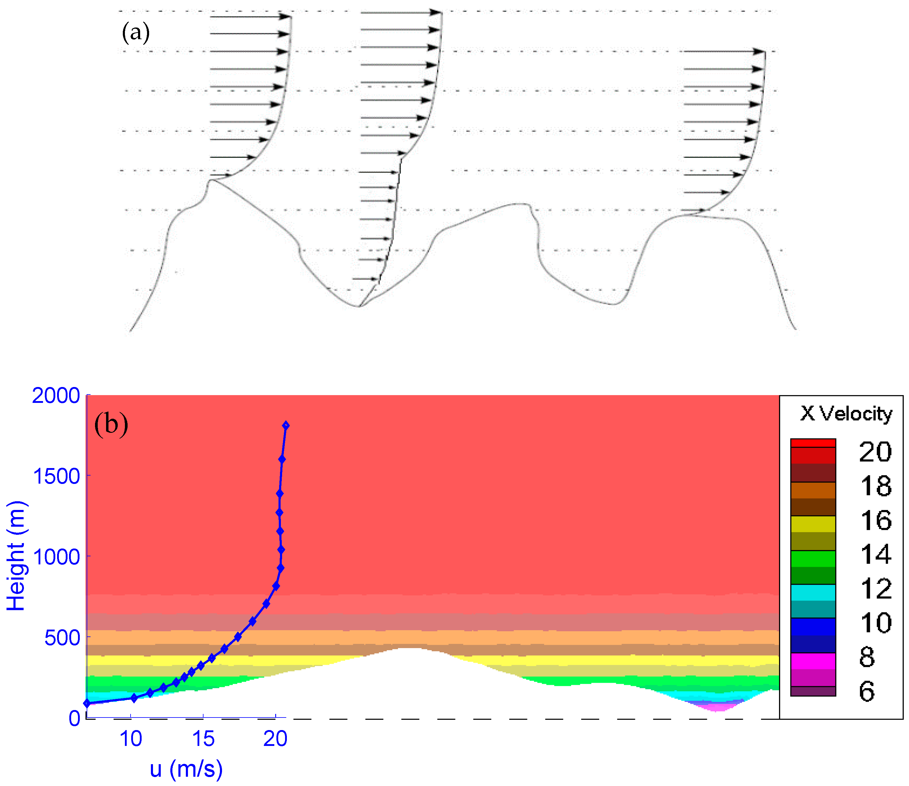
The CFD model usually uses the extrapolation coupling method [21]. The NWP wind profile is extrapolated between the altitude of the lowest level of NWP profile and the ground level in the CFD grid using extrapolation, as shown in Figure 3. This method uses a single NWP wind profile to define the CFD boundary condition of an entire inlet boundary, which may be not a suitable boundary condition for the complex terrain. The sketch map of the extrapolation method behavior is illustrated in Figure 3a. The u component of the CFD wind speed on an entire boundary, for example, is given in Figure 3b. Using extrapolation, a single NWP profile (blue curve at 0 km on the horizontal axis) was extrapolated on the CFD boundary.
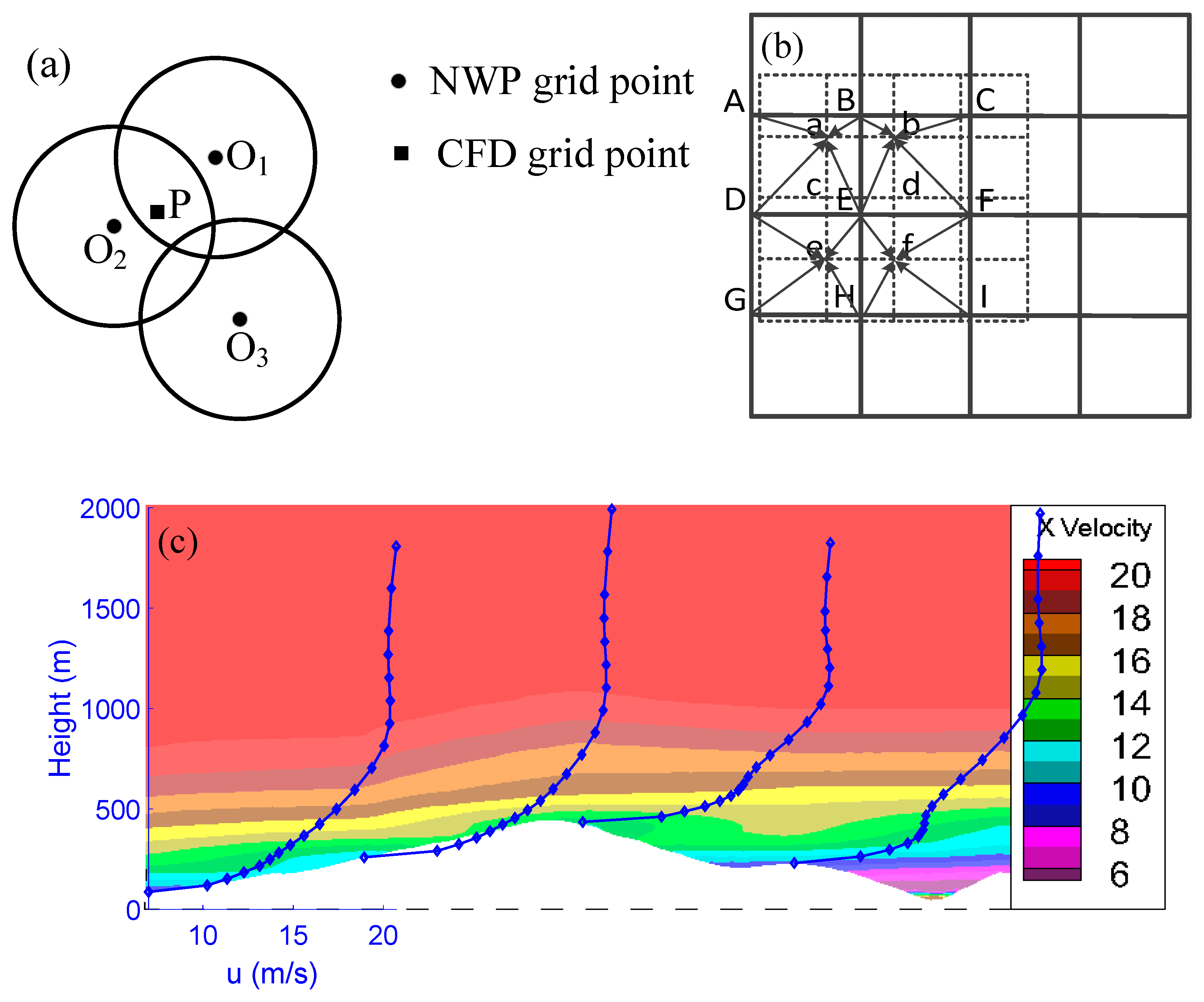
In order to calculate a CFD boundary condition suitable for complex terrain, we adopted the Cressman interpolation method [22] to couple the NWP and CFD models. Wind speed of the CFD grid point can be calculated as the combination of nearby NWP grid points’ data using Cressman interpolation, as shown in Figure 4. The result of using this method may be more realistic and suitable for complex terrain. Figure 4a shows an example of the Cressman interpolation method, the NWP data O1 and O2 influence the CFD grid point P, but O3 does not. Figure 4b shows the sketch map of imposing NWP grid points on a CFD boundary, A–I represent NWP grid points, a–f represent CFD grid points. By setting an appropriate value for the horizontal and vertical influence radius, each CFD grid point can be calculated by the nearby NWP grid points. The u component of the CFD wind speed on an entire boundary, for example, is shown in Figure 4c. Using Cressman interpolation, five NWP wind profiles (blue curves at 0 km, 1 km, 2 km, 3 km, and 4 km on the horizontal axis) were interpolated on the CFD boundary.
The interpolated value is weighted only depending on the distance between the CFD and NWP models’ grid points. Therefore, the interpolated wind components can be calculated as follows:
V i n t e r p o l a t e = i = 1 n N W P V i W i / i = 1 n N W P W i
n N W P is the number of NWP grid points nearby, the weighting function W i is the function of the distance between the CFD grid point (coordinates x v a l u e , y v a l u e , and z v a l u e ) and nearby NWP grid points (coordinates x i , y i , and z i ):
W i = w x y · w z = r L 2 d x y 2 r L 2 + d x y 2 · ( 1 | d z | r z )
d x y 2 = ( x v a l u e x i ) 2 + ( y v a l u e y i ) 2
| d z | = | z v a l u e z i |
r L and r z are the horizontal and vertical radius influenced by the NWP grid points, respectively. r L is set as 600 m, and r z is set as 100 m in this research.

3.2. Data Assimilation for CFD Model

As we know, data assimilation is widely used in NWP models, in which meteorological observation data enter the analysis cycles and models’ forecasts. There has already been a lot of research looking at the data assimilation in NWP models [11,12,23,24]. However, very few studies have been concerned about data assimilation for the CFD models.
In this work, a preliminary study was conducted on the data assimilation for the CFD model. The Newtonian relaxation technique, nudging, was utilized to assimilate the observations into the CFD model simulation. It works by adding a term to the forecast equation that can nudge the solution towards the observation data [23]. For example, the velocity equation that nudging used can be written as follows:
( u i ) t + u j ( u i ) x j = ν x i ( u i x j ) 1 ρ p x i + ( u o b s u τ u )   W ( x , y , z , t )
u o b s is the observed velocity that interpolated at the CFD grid points, u is the predicted velocity of the previous time step, τ u is the nudging coefficient, and W ( x , y , z , t ) is the Cressman type weighting function. τ u is usually chosen based on the variables and empirical consideration. W ( x , y , z , t ) is widely used in NWP models, but it does not vary in time in the CFD simulations since the time integration is very small. In the same way, other forecast equations can be modified by nudging.
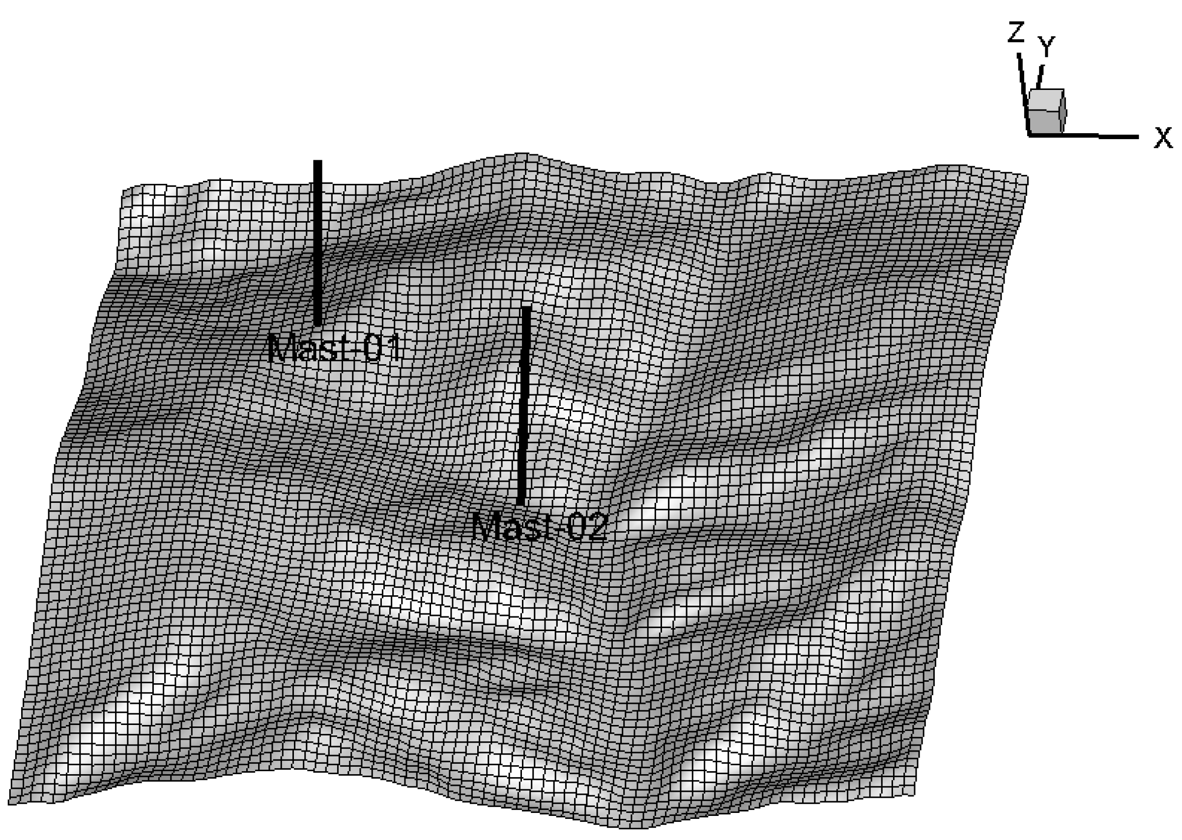
A preliminary study of data assimilation for the CFD model was conducted in this work. The NWP wind profile at Mast-01 was assimilated into the CFD model, to see whether the CFD solutions at two sites (Mast-01, Mast-02) are nudged toward the original NWP data. Figure 5 shows the sites of Mast-01 and Mast-02 in the CFD domain.

4. Results and Discussion

4.1. Coupling Methods

We analyzed the coupling methods for the CFD simulation over a 3-day period in May 2018. Two coupling methods, extrapolation and Cressman interpolation, were used to calculate the boundary condition for the CFD simulation.
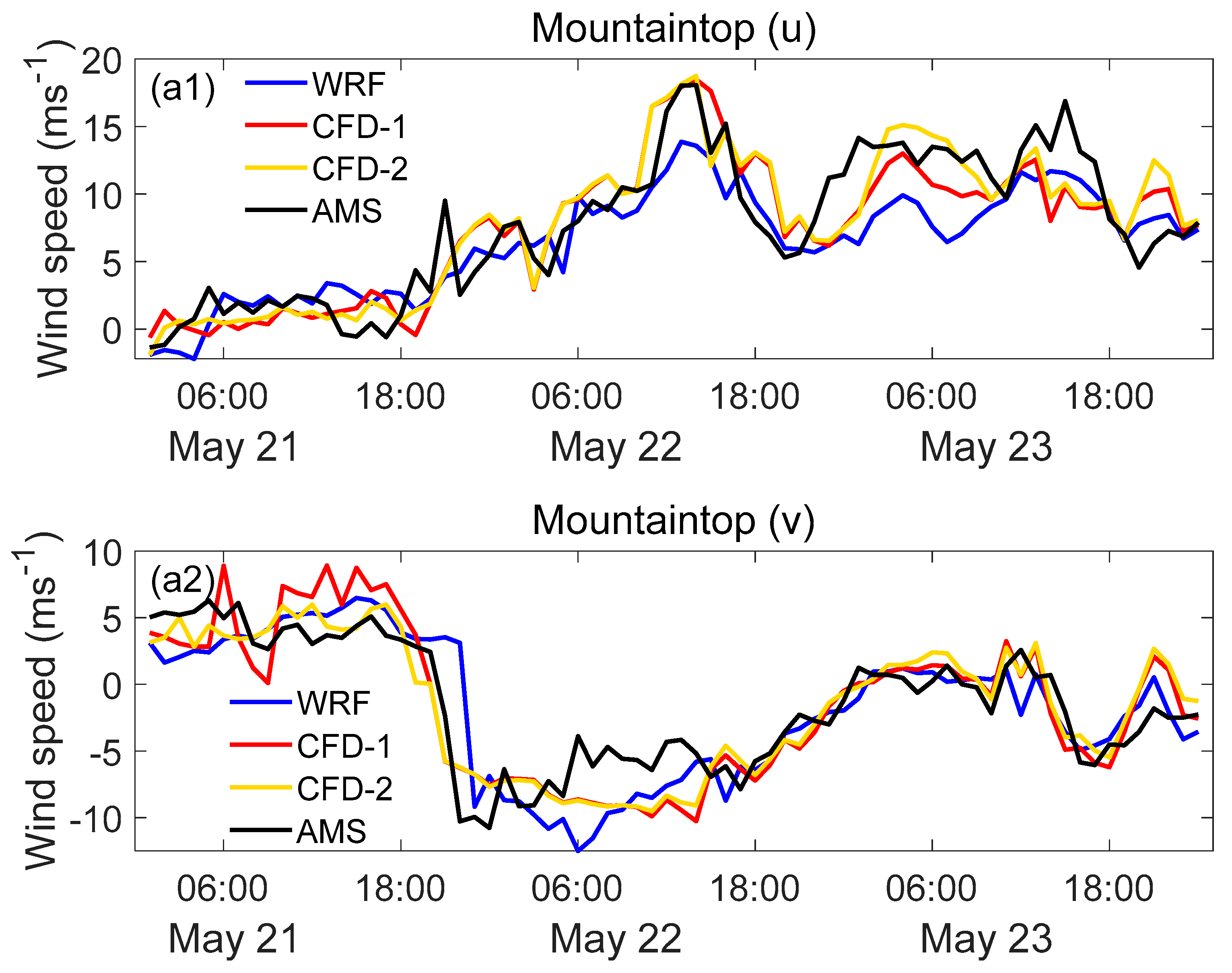
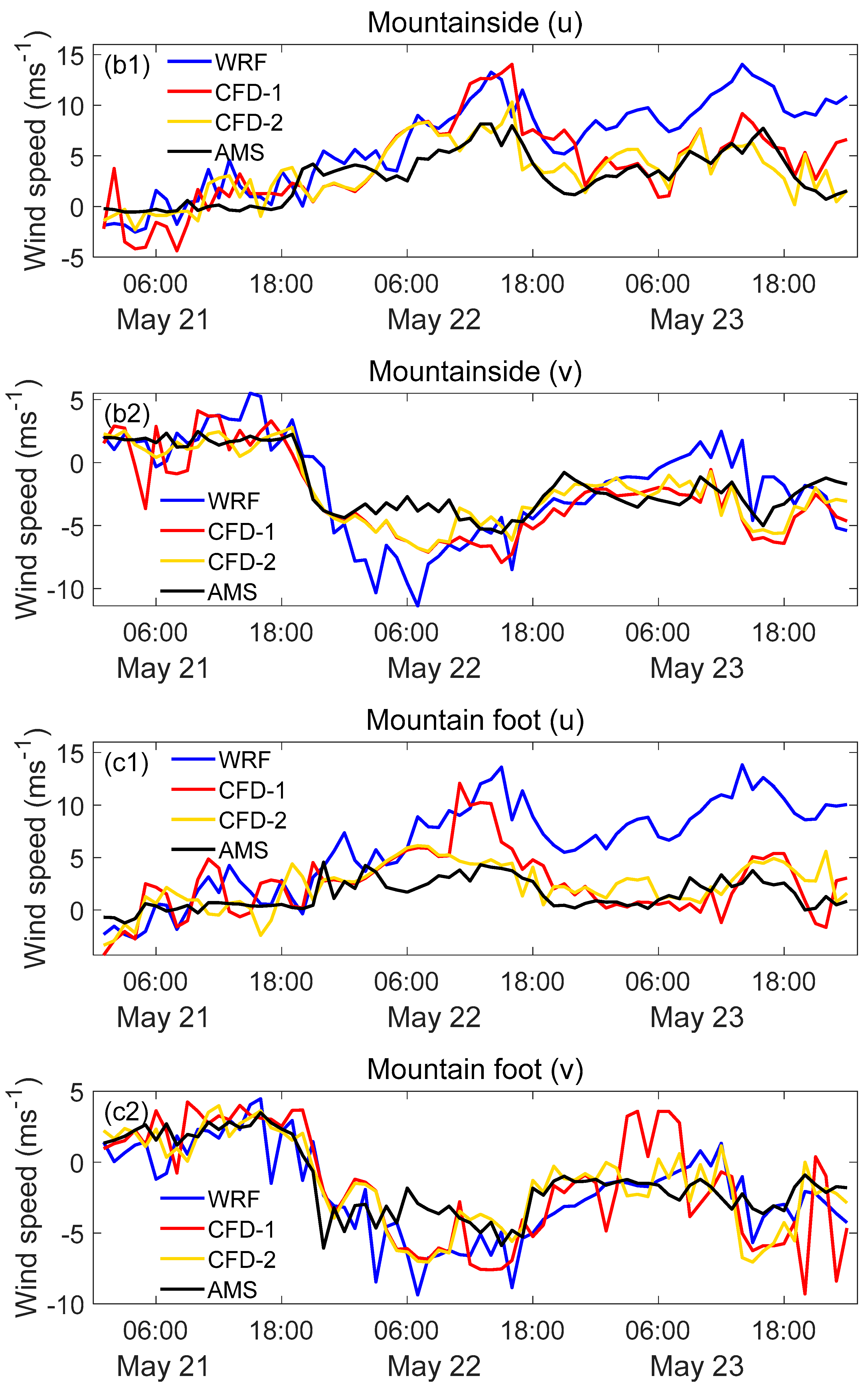
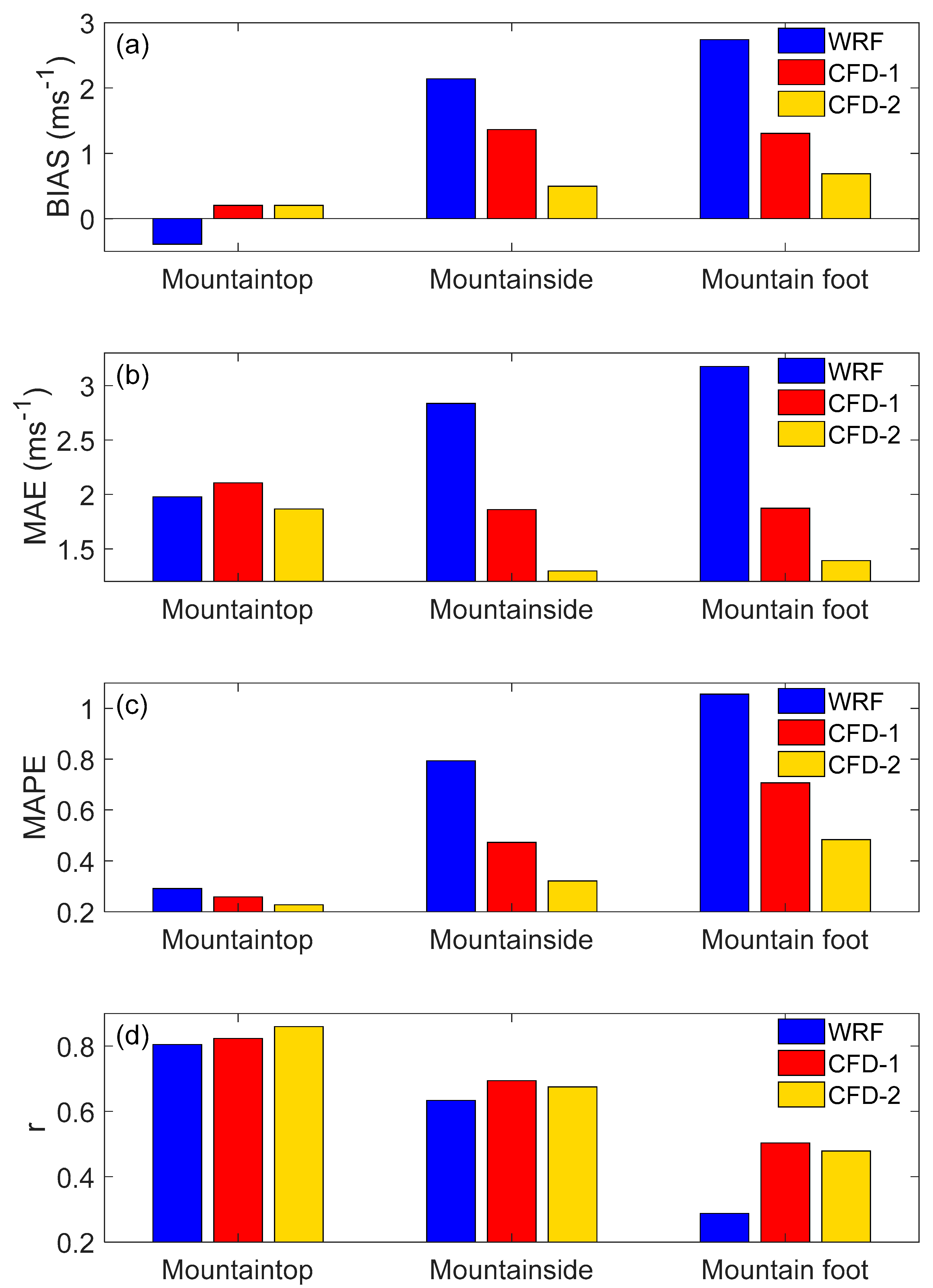
Figure 6 displays the time series of simulated wind for different numerical models: WRF, CFD using the extrapolation coupling method (CFD-1), and the Cressman coupling method (CFD-2). The observations measured by AMS-1, AMS-2, and AMS-3 are used for the validation of these models. Figure 7 shows the calculated results of the sensitivity analysis for these models’ simulations, four indexes are considered: systematic deviations from expected values (BIAS), mean absolute error (MAE), mean absolute percentage error (MAPE), and temporal correlation coefficient (r).
Firstly, in comparison with the WRF model, the CFD model has the better performance in simulating wind flow. For example, the BIAS indicates greater underestimation for the WRF model (~2.142 ms−1 on the mountainside), with slight overestimation for the CFD-1 model (~1.364 ms-1 on the mountainside) and the CFD-2 model (~0.496 ms−1 on the mountainside). Similarly, MAE, MAPE, and r results reflect remarkable improvement from WRF to CFD model simulation. r increases from about 28.8% for the WRF simulation to about 50.4% for the CFD-1 simulation and 47.9% for the CFD-2 simulation at the mountain foot.
Secondly, in comparison with the CFD model using the extrapolation coupling method (CFD-1), the CFD model using the Cressman coupling method (CFD-2) has the better performance in wind field simulation. For instance, BIAS decreases from about 1.307 ms−1 for the CFD-1 model to 0.686 ms−1 for the CFD-2 model at the mountain foot. MAPE decreases from about 47.4% for the CFD-1 model to about 32.2% for the CFD-2 model on the mountainside.
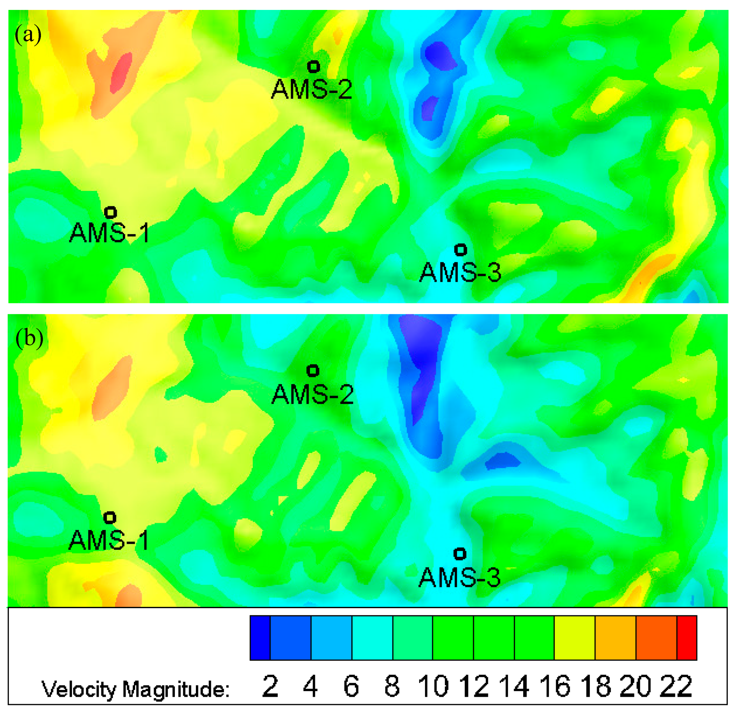
To visually evaluate the performance of different coupling methods on wind field simulation, Figure 8 depicts the partial distribution of wind velocity near ground simulated by the CFD-1 and CFD-2 models. From Figure 8, there are some differences in the wind field between the CFD-1 and CFD-2 simulations, and the CFD-2 model has the better performance. For instance, wind velocity on the mountainside from the CFD-2 simulation (~11.45 ms−1) is closer to the observation data (~9.21 ms−1 for AMS-2) than the CFD-1 simulation (~14.22 ms−1). Wind velocity at the mountain foot from CFD-2 simulation (~7.11 ms−1) is closer to the observation data (~6.14 ms−1 for AMS-3) than the CFD-1 simulation (~9.14 ms−1). Therefore, the Cressman coupling method may be more suitable for wind field simulation over complex terrain.
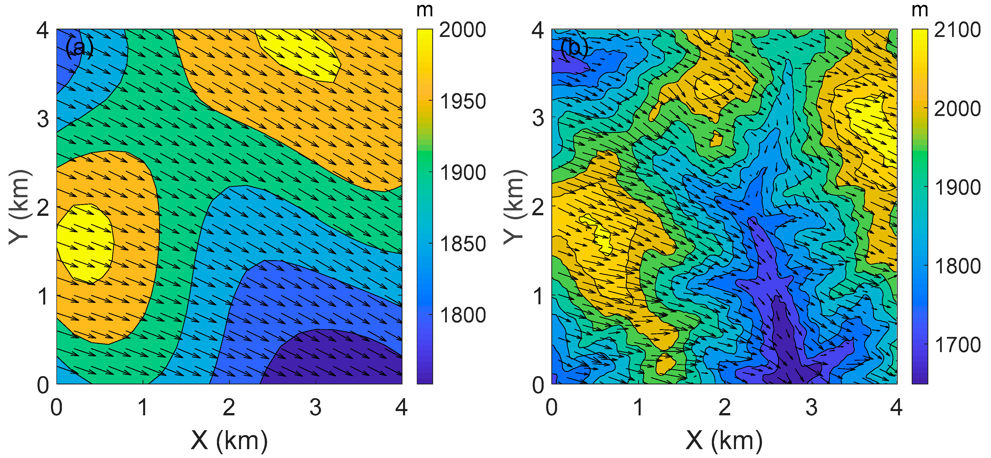
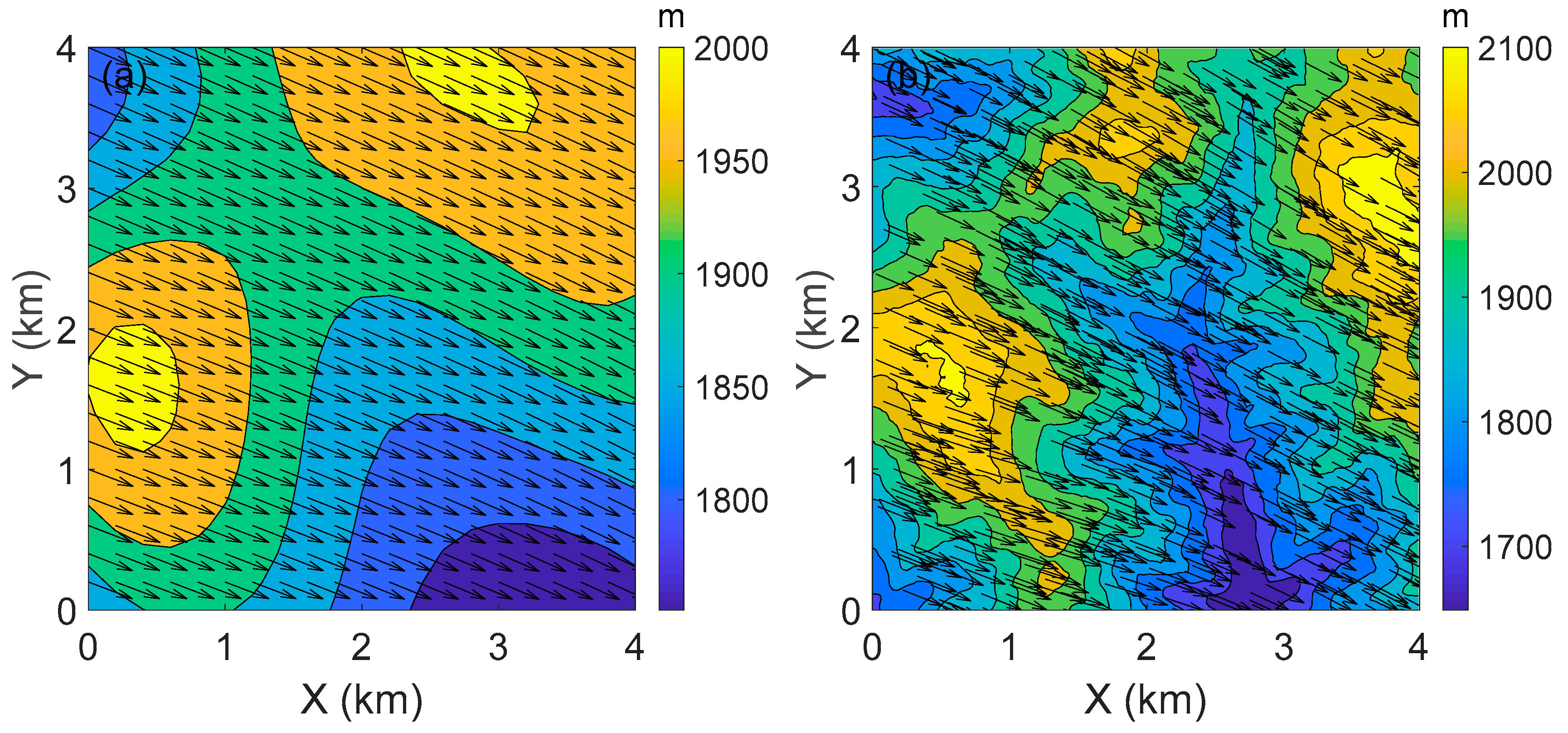
Figure 9 and Figure 10 show the micro-scale wind field simulated by the CFD model, and which is compared with the WRF simulation. From Figure 9, it can be seen that the wind flow from the WRF and CFD simulations are similar on the whole, as the prevailing wind direction in both simulations is northwest. However, some details of the wind field from the two simulations are extremely different. The wind fields from the WRF simulation are relatively smooth. On the contrary, wind fields from the CFD simulations show more heterogeneity. The difference in the near-ground wind field between the WRF and CFD simulations can be partially due to the great difference between the terrains of these two models. From Figure 10, it can be observed that the wind flow from the WRF and CFD simulations are basically the same. The main reason is that the effect of terrain on the wind is small at higher altitudes.

4.2. Data Assimilation

To further improve the NWP/CFD model performance, a data assimilation system, nudging, is applied in the CFD model. The implementation of the data assimilation procedure was carried out on 22 May 2018 at 16:00 UTC. The idea was to assimilate the WRF profile data of Mast-01 into the CFD model, and to see whether the CFD solutions at two sites (Mast-01, Mast-02) were nudged toward the original WRF data.
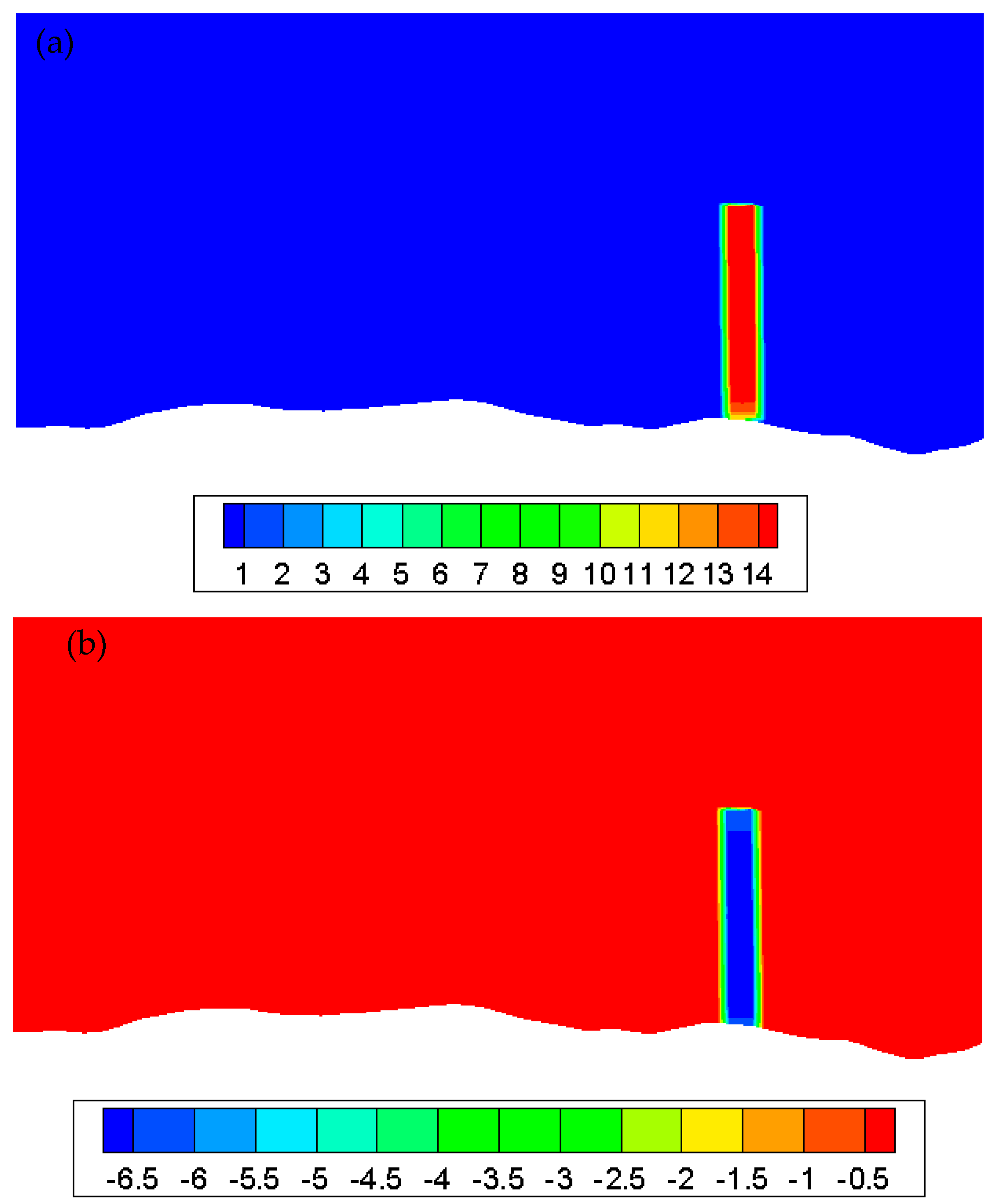
Firstly, the velocities u o b s in Equation (5) were interpolated near Mast-01 by using the Cressman interpolation method, as shown in Figure 11, and the horizontal radius and vertical radius influenced by the WRF grid points were set as 100 m and 50 m, respectively. Then, the Cressman type weighting function, W ( x , y , z , t ) from Equation (5) was computed. Figure 12 shows the cross-section (horizontal and vertical) of W ( x , y , z , t ) applied at an observed point. The value of the weighting function decreased gradually as the distance from the observed point increased.
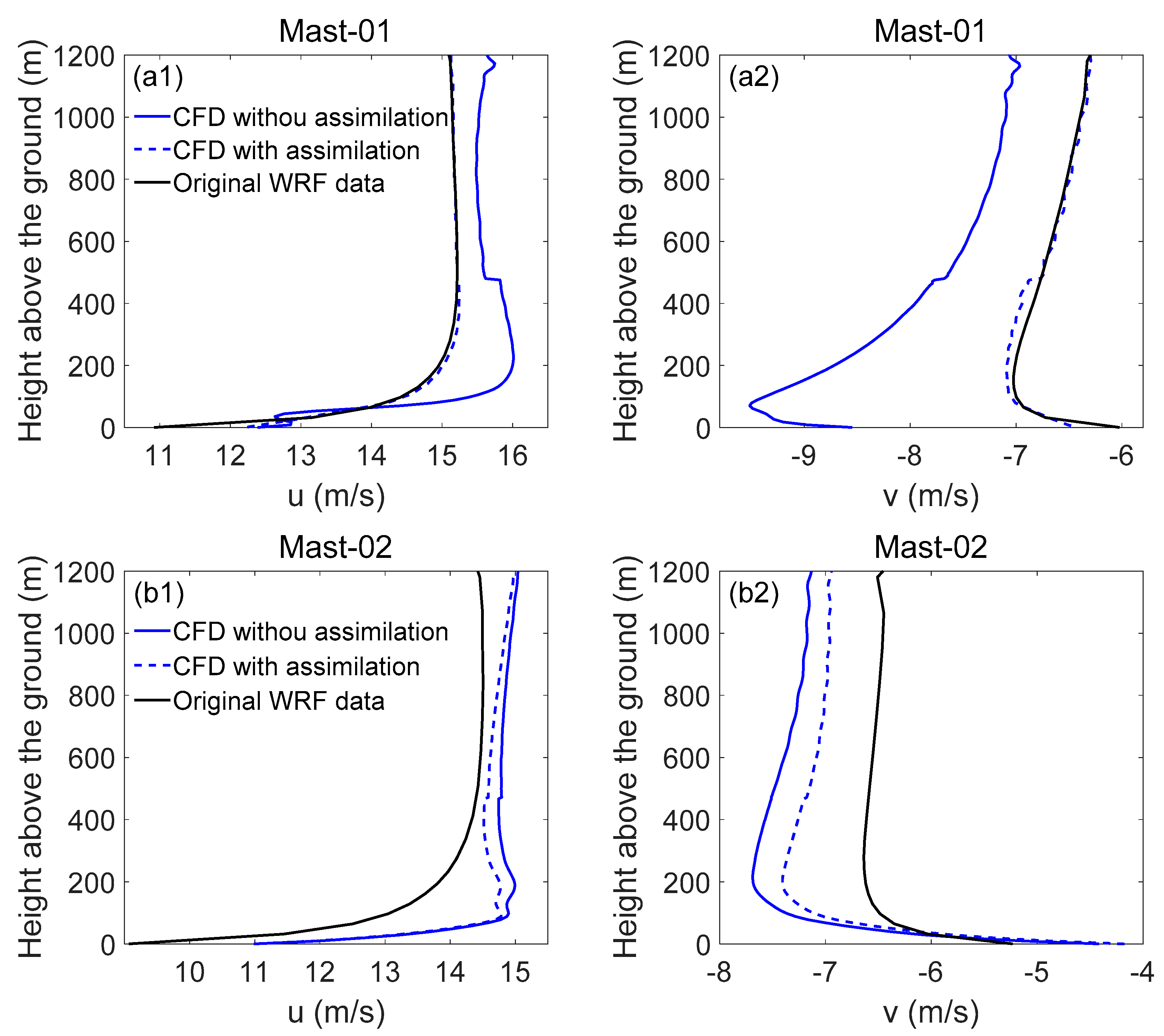
Figure 13 shows the influence of data assimilation on wind simulation near the two sites (AMS-01, AMS-02) chosen for study. The solid blue curves refer to the CFD simulation without assimilation, the blue dotted curves signify the CFD simulation with assimilation, and the solid black curves represent the original WRF wind data at AMS-01 and AMS-02. Our goal is to nudge the CFD solution towards the original WRF wind data from the CFD without assimilation. Note that CFD wind data at Mast-01 is nudged towards the original WRF data by the influence of data assimilation. Following the control equations of fluid mechanics, the CFD wind data at the Mast-02 site is modified somewhat towards the original WRF wind data.
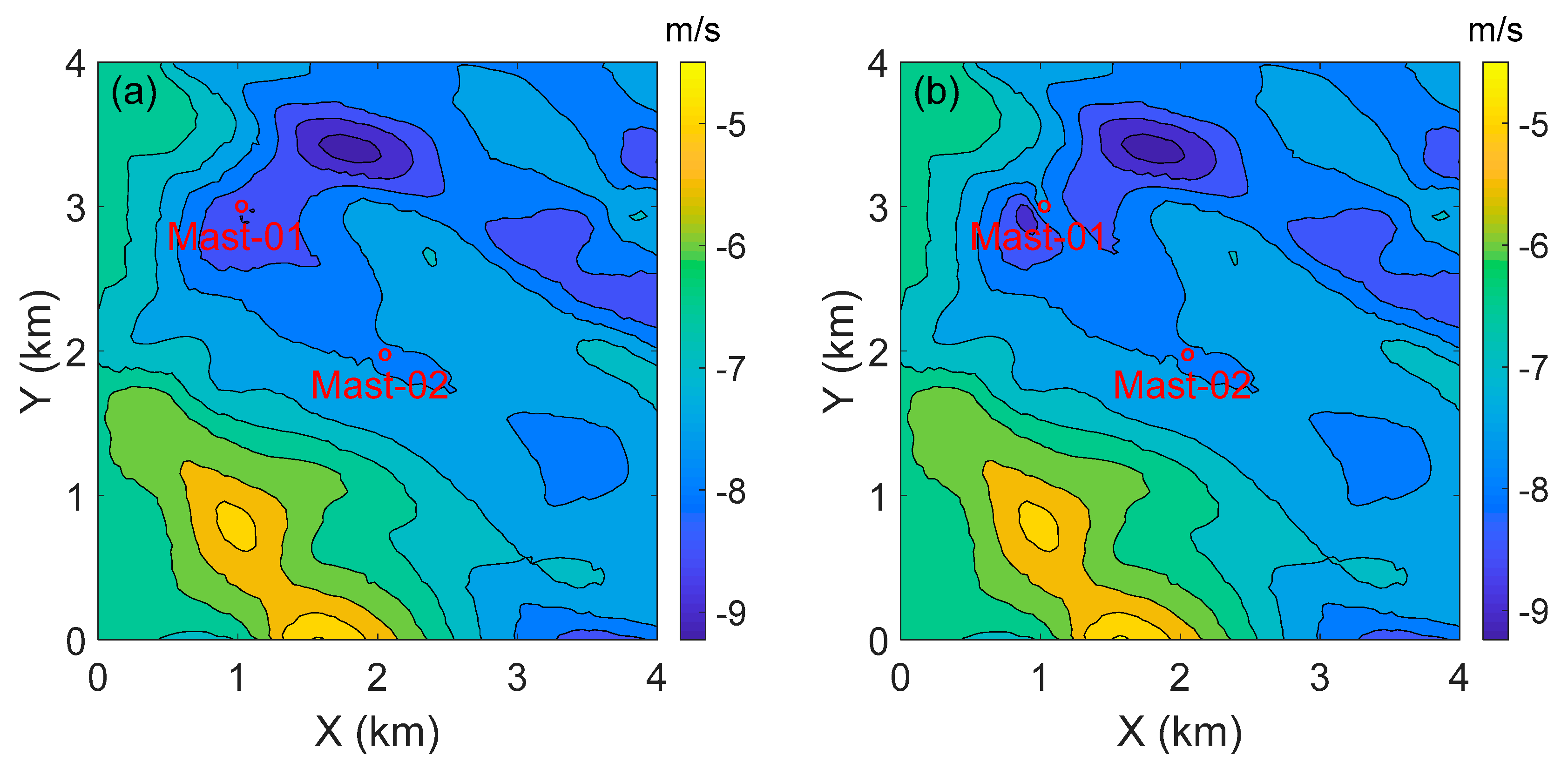
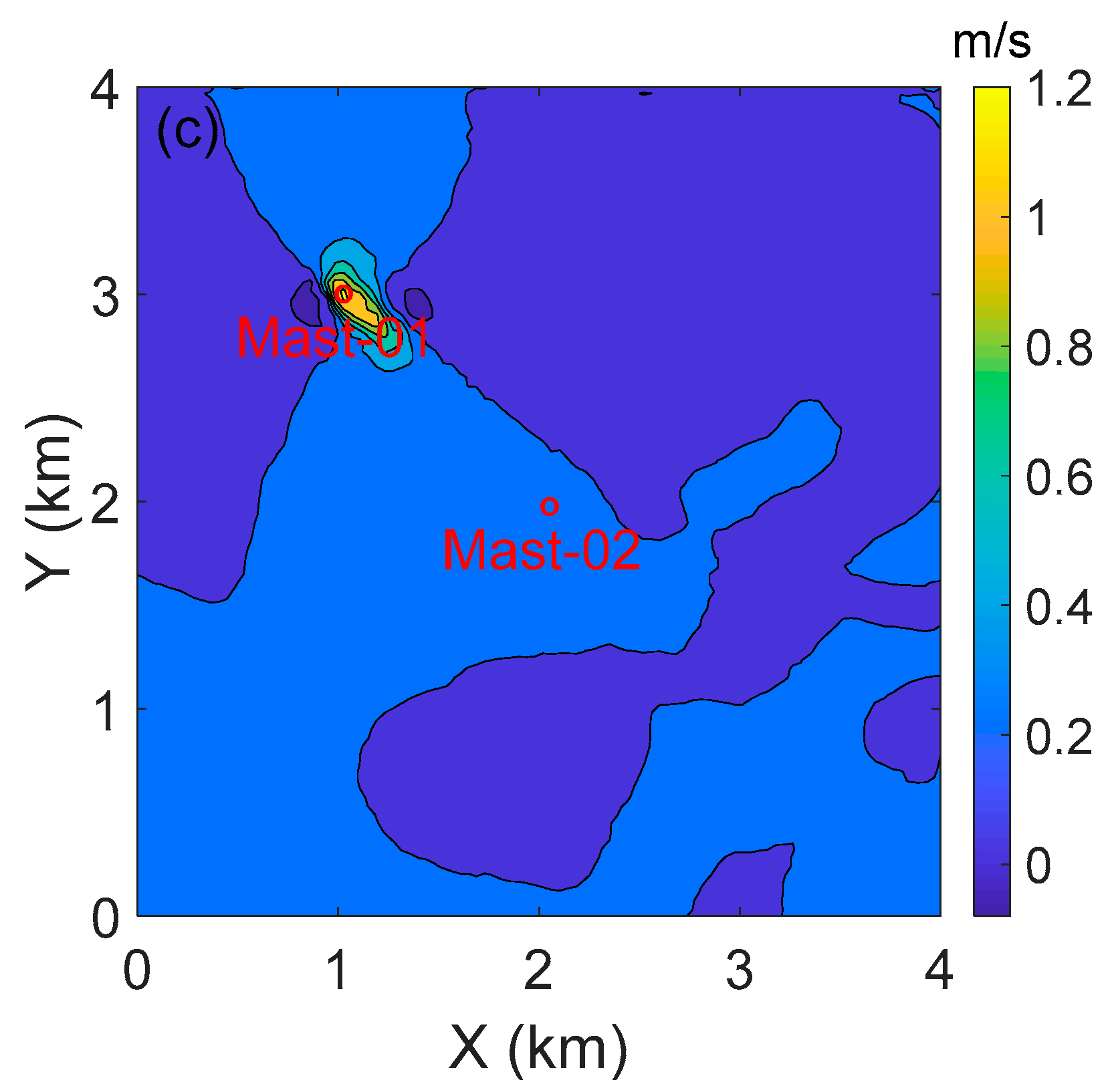
Figure 14 and Figure 15 show the influence of data assimilation on the wind velocity components at altitude of 400 m. Figure 14a–c illustrate the CFD model simulation without assimilation, the CFD model simulation with assimilation, and the difference between the CFD simulation with and without assimilation, respectively. It can be seen that the CFD simulation with data assimilation (Figure 14b and Figure 15b) has adjusted the wind flow in both the u and v components in comparison with the CFD simulation without data assimilation (Figure 14a and Figure 15a). From the difference between the CFD model simulation with and without assimilation (Figure 14c and Figure 15c), it is quite obvious that the wind field upstream and downstream of the assimilation site was modified by nudging.
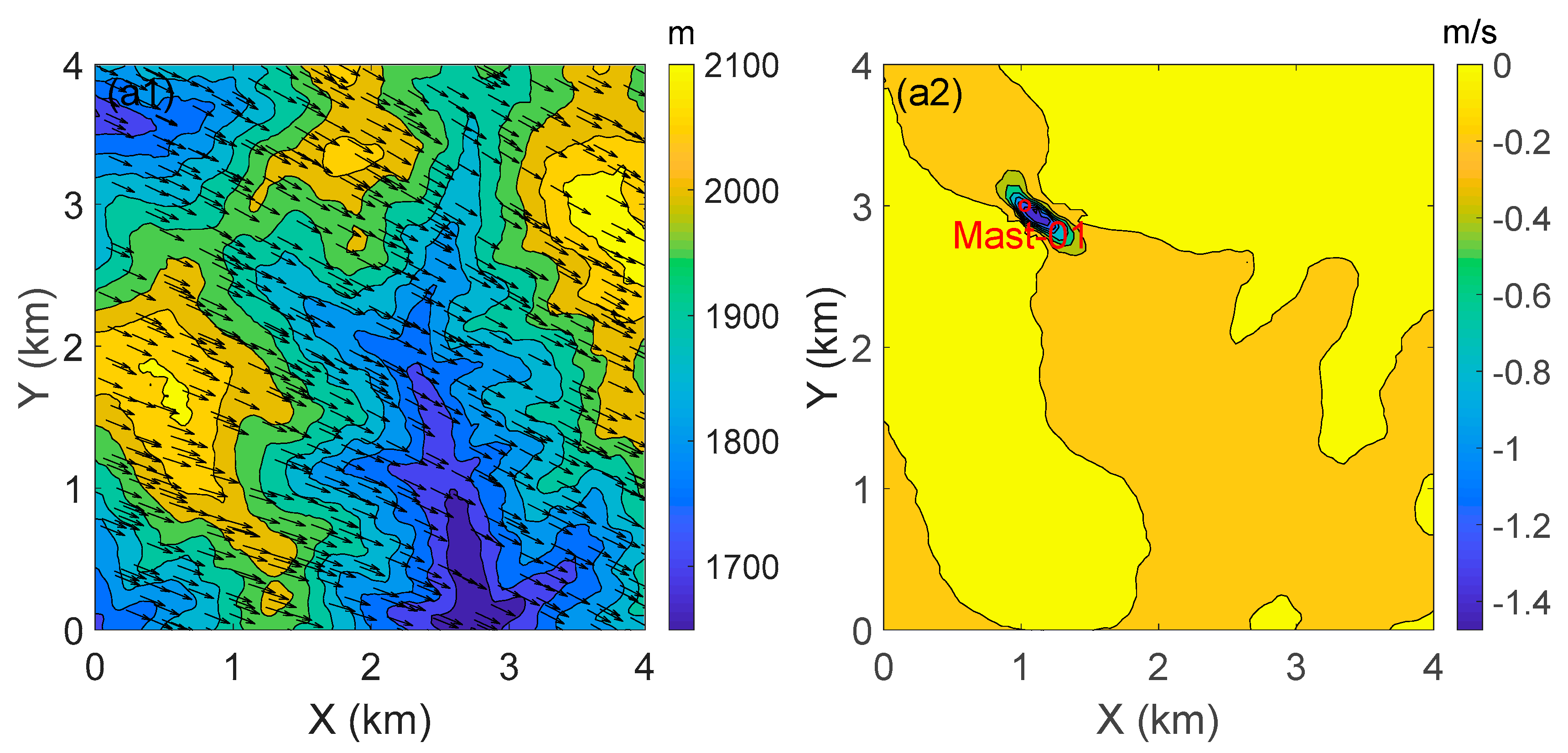
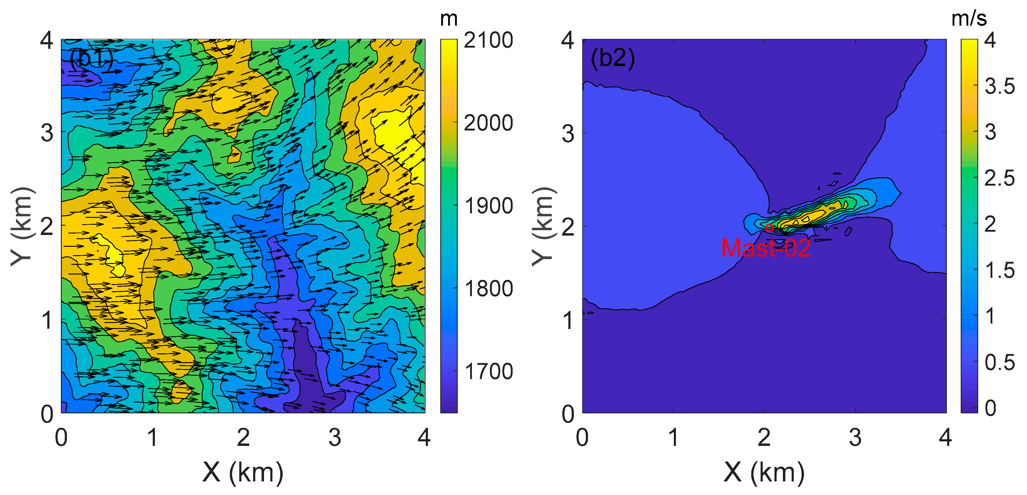
Figure 16 shows the relationship between wind direction and the impact area of data assimilation. Figure 16 (a1,a2) depicts the wind vectors and the difference in wind velocity between the CFD model simulation with and without assimilation at 400 m altitude, on 22 May 2018 at 16:00 UTC. From the figure, the wind direction is northwest, and the impact of nudging seems elongated along a NW–SE axis. Figure 16 (b1,b2) depicts the wind vectors and the difference in wind velocity between the CFD model simulation with and without assimilation at 400 m altitude, on 23 May 2018 at 13:00 UTC. From the figure, the wind direction is west, and the impact of nudging seems elongated along the W–E axis. Therefore, it can be observed that the wind field upstream and downstream of the assimilation site was modified by nudging.

5. Conclusions

Understanding the details of the wind field within the atmospheric boundary layer is very important for siting wind power plants in wind energy industries. Coupling NWP and CFD models has proven successful in simulating micro-scale wind fields. Our goal is to improve the NWP/CFD model performance by developing a new coupling method between two models and applying a data assimilation system in the CFD model.
To develop the coupling method, the Cressman interpolation were used to impose NWP model wind on CFD boundaries. In comparison with the traditional coupling method, the CFD model using the Cressman interpolation has the better performance in wind field simulation over complex terrain. For example, the index BIAS decreases from about 1.307 ms−1 to 0.686 ms−1 at the mountain foot, and MAPE decreases from about 47.4% to 32.2% on the mountainside. An NWP/CFD model with an improved coupling method may capture the details of micro-scale wind fields more accurately. Therefore, the Cressman interpolation coupling method may be effective at improving the NWP/CFD model performance. Due to the lack of observation sites and data, only three sites and three days of simulation are considered in this paper. More work should be done in the next step: test the coupling methods again when more observations are available for comparison or test the coupling methods in other places with complex terrain.
To further improve the NWP/CFD model performance, a data assimilation system, nudging, was applied in the CFD model. A preliminary experiment of data assimilation for CFD model was carried out, and the CFD solution was nudged towards the assimilated data. The wind field upstream and downstream of the assimilation site was modified by nudging.
In this research, a method to apply assimilation of observations into the CFD model was explored. Preliminary results of data assimilation indicate that assimilating the NWP profile into the CFD simulation can nudge the wind field towards that of NWP while retaining the mass consistency of CFD model. It can be seen that such data assimilation is feasible and deserves further research. Using data assimilation, the NWP/CFD model performance may be further improved by cooperating observation data. More work can be conducted in the next steps: test the appropriate nudging coefficient, tune the influence radius of the weighting function, test the nudging technique when more observations are available for comparison, and so on.

Author Contributions

Writing—original draft preparation, S.L.; supervision, X.S.; data curation, R.Z.; formal analysis, C.Z.

Funding

This research was funded by the National Natural Science Foundation of China, grant number 41575020.

Conflicts of Interest

The authors declare no conflict of interest. The funders had no role in the design of the study; in the collection, analyses, or interpretation of data; in the writing of the manuscript, or in the decision to publish the results.

References

  1. Mohagheghi, E.; Gabash, A.; Li, P. A Framework for Real-Time Optimal Power Flow under Wind Energy Penetration. Energies 2017, 10, 535. [Google Scholar] [CrossRef]
  2. Blocken, B.; van der Hout, A.; Dekker, J.; Weiler, O. CFD simulation of wind flow over natural complex terrain: Case study with validation by field measurements for Ria de Ferrol, Galicia, Spain. J. Wind Eng. Ind. Aerod. 2015, 147, 43–57. [Google Scholar] [CrossRef]
  3. Sumner, J.; Watters, C.S.; Masson, C. CFD in wind energy: The virtual, multiscale wind tunnel. Energies 2010, 3, 989–1013. [Google Scholar] [CrossRef]
  4. Dhunny, A.Z.; Lollchund, M.R.; Rughooputh, S. Wind energy evaluation for a highly complex terrain using Computational Fluid Dynamics (CFD). Renew. Energy 2017, 101, 1–9. [Google Scholar] [CrossRef]
  5. Castellani, F.; Burlando, M.; Taghizadeh, S.; Astolfi, D.; Piccioni, E. Wind energy forecast in complex sites with a hybrid neural network and CFD based method. Energy Procedia 2014, 45, 188–197. [Google Scholar] [CrossRef]
  6. Dhunny, A.Z.; Lollchund, M.R.; Rughooputh, S. A high-resolution mapping of wind energy potentials for Mauritius using Computational Fluid Dynamics (CFD). Wind Struct. 2015, 20, 565–578. [Google Scholar] [CrossRef]
  7. Tewari, M.; Kusaka, H.; Chen, F.; Coirier, W.J.; Kim, S.; Wyszogrodzki, A.A.; Warner, T.T. Impact of coupling a microscale computational fluid dynamics model with a mesoscale model on urban scale contaminant transport and dispersion. Atmos. Res. 2010, 96, 656–664. [Google Scholar] [CrossRef]
  8. Zajaczkowski, F.J.; Haupt, S.E.; Schmehl, K.J. A preliminary study of assimilating numerical weather prediction data into computational fluid dynamics models for wind prediction. J. Wind Eng. Ind. Aerod. 2011, 99, 320–329. [Google Scholar] [CrossRef]
  9. Li, L.; Chan, P.W. Numerical simulation study of the effect of buildings and complex terrain on the low-level winds at an airport in typhoon situation. Meteorol. Z. 2012, 21, 183–192. [Google Scholar] [CrossRef]
  10. Bindu, H.H.; Ratnam, M.V.; Yesubabu, V.; Rao, T.N.; Kesarkar, A.; Naidu, C.V. Characteristics of cyclone generated gravity waves observed using assimilated WRF model simulations over Bay of Bengal. Atmos. Res. 2016, 180, 178–188. [Google Scholar] [CrossRef]
  11. Barker, D.M.; Huang, W.; Guo, Y.R.; Bourgeois, A.J.; Xiao, Q.N. A three-dimensional variational data assimilation system for mm5: Implementation and initial results. Mon. Weather Rev. 2004, 132, 897–914. [Google Scholar] [CrossRef]
  12. Huang, X.Y.; Xiao, Q.; Barker, D.M.; Zhang, X.; Michalakes, J.; Huang, W.; Henderson, T.; Bray, J.; Chen, Y.; Ma, Z.; et al. Four-Dimensional Variational Data Assimilation for WRF: Formulation and Preliminary Results. Mon. Weather Rev. 2009, 137, 299–314. [Google Scholar] [CrossRef] [Green Version]
  13. Grell, G.A.; Peckham, S.E.; Schmitz, R.; McKeen, S.A.; Frost, G.; Skamarock, W.C.; Eder, B. Fully coupled ‘online’ chemistry within the WRF model. Atmos. Environ. 2005, 39, 6957–6975. [Google Scholar] [CrossRef]
  14. Li, Y.; Lu, G.; Wu, Z.; He, H.; Shi, J.; Ma, Y.; Weng, S. Evaluation of Optimized WRF Precipitation Forecast over a Complex Topography Region during Flood Season. Atmosphere 2016, 7, 145. [Google Scholar] [CrossRef]
  15. Pennelly, C.; Reuter, G. Verification of the Weather Research and Forecasting Model when Forecasting Daily Surface Conditions in Southern Alberta. Atmosphere 2017, 55, 31–41. [Google Scholar] [CrossRef]
  16. Jasak, H. OpenFOAM: Open source CFD in research and industry. Int. J. Nav. Arch. Ocean 2009, 1, 89–94. [Google Scholar] [Green Version]
  17. Flores, F.; Garreaud, R.; Muñoz, R.C. CFD simulations of turbulent buoyant atmospheric flows over complex geometry: Solver development in OpenFOAM. Comput. Fluids 2013, 82, 1–13. [Google Scholar] [CrossRef]
  18. Mangani, L.; Darwish, M.; Moukalled, F. An OpenFOAM pressure-based coupled CFD solver for turbulent and compressible flows in turbomachinery applications. Numer. Heat Transf. B Fund. 2016, 69, 413–431. [Google Scholar] [CrossRef]
  19. Reddy, G.O.; Kumar, N.; Sahu, N.; Singh, S.K. Evaluation of automatic drainage extraction thresholds using ASTER GDEM and Cartosat-1 DEM: A case study from basaltic terrain of Central India. Egypt. J. Remote Sens. Space Sci. 2017, 21, 95–104. [Google Scholar] [CrossRef]
  20. Haga, T.; Kuzuu, K.; Takaki, R.; Shima, E. Assessment of an Unstructured CFD Solver for RANS Simulation on Body-Fitted Cartesian Grids. In Proceedings of the Aerospace Sciences Meeting 2014, National Harbor, MD, USA, 13–17 January 2014. [Google Scholar]
  21. Laporte, L.; Dupont, É.; Carissimo, B.; Musson-Genon, L.; Sécolier, C. Atmospheric CFD simulations coupled to mesoscale analyses for wind resource assessment in complex terrain. In Proceedings of the European Wind Energy Conference, Marseille, France, 16 March 2009. [Google Scholar]
  22. Wikle, C.K. Atmospheric Modeling, Data Assimilation, and Predictability. Technometrics 2002, 47, 521. [Google Scholar] [CrossRef]
  23. Warner, T.T. Numerical Weather and Climate Prediction; Cambridge University Press: Cambridge, UK, 2011; pp. 504–526. [Google Scholar]
  24. Dee, D.P.; Uppala, S.M.; Simmons, A.J.; Berrisford, P.; Poli, P.; Kobayashi, S.; Andrae, U.; Balmaseda, M.A.; Balsamo, G.; Bauer, D.P.; et al. The era-interim reanalysis: Configuration and performance of the data assimilation system. Q. J. R. Meteorol. Soc. 2011, 137, 553–597. [Google Scholar] [CrossRef]
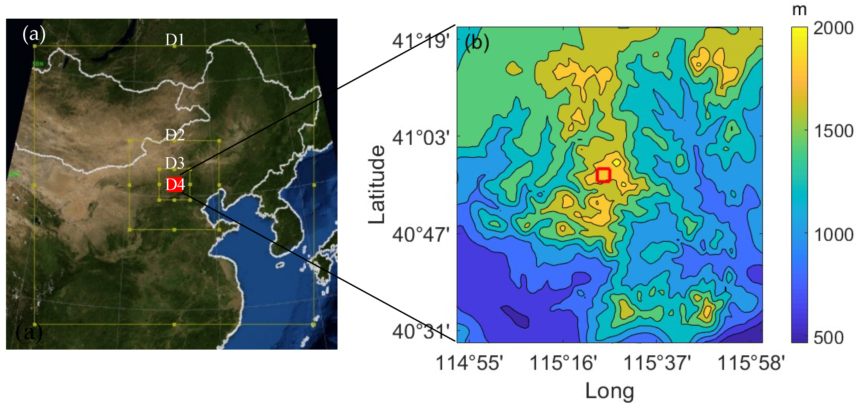
Figure 1. Study area of the Weather Research and Forecasting (WRF) simulation: (a) the WRF domain location and configuration around Chongli Montain; (b) terrain height in domain D4, and the Computational Fluid Dynamics (CFD) domain configuration (red box).
Energies 12 02549 g001
Figure 2. The sketch map of the CFD simulation configuration: (a) terrain height of the CFD domain; (b) 3D terrain modeling of the CFD domain, the red dots indicate the locations of the automatic meteorological stations (AMS); (c) the body-fitted hexahedral grid system used in the CFD domain.
Energies 12 02549 g002
Figure 3. Extrapolation coupling method: (a) sketch map of extrapolation coupling on complex terrain; (b) the u component (m/s) of the CFD wind speed on the western boundary of the CFD domain. On the boundary, the horizontal axis represents width (0–4 km) of the CFD domain, and the vertical axis represents height (0–2 km). Using extrapolation, a single NWP profile (blue curve at 0 km on the horizontal axis) was extrapolated on the CFD boundary.
Energies 12 02549 g003
Figure 4. Cressman interpolation method: (a) sketch map of Cressman interpolation; (b) sketch map of imposing NWP grid points on a CFD boundary, A–I represent NWP grid points, a–f represent CFD grid points; (c) the u component (m/s) of the CFD wind speed on the western boundary of the CFD domain. On the boundary, the horizontal axis represents width (0–4 km) of the CFD domain, and the vertical axis represents height (0–2 km). Using Cressman interpolation, five NWP wind profiles at 0 km, 1 km, 2 km, 3 km, and 4 km on the horizontal axis (blue curves) were interpolated on the CFD boundary.
Energies 12 02549 g004
Figure 5. The sites of Mast-01 (coordinates x = 1000, y =3000) and Mast-02 (coordinates x = 2000, y = 2000) in the CFD domain.
Energies 12 02549 g005
Figure 6. Time series of simulated wind for different numerical models: WRF, CFD-1, and CFD-2: (a1,a2) wind flow on the mountaintop; (b1,b2) wind flow on the mountainside; (c1,c2) wind flow at the mountain foot.
Energies 12 02549 g006aEnergies 12 02549 g006b
Figure 7. Calculated results of the sensitivity analysis for different models’ simulations, four indexes ((a) systematic deviations from expected values (BIAS), (b) mean absolute error (MAE), (c) mean absolute percentage error (MAPE), and (d) temporal correlation coefficient (r)) are considered.
Energies 12 02549 g007
Figure 8. Partial distribution of wind velocity (m/s) near ground simulated by the CFD-1 (a) and CFD-2 (b) models, on 22 May 2018 at 16:00 UTC.
Energies 12 02549 g008
Figure 9. The topography (m) and simulated wind (vectors) at a height of 10 m: (a) WRF simulation; (b) CFD simulation.
Energies 12 02549 g009
Figure 10. The topography (m) and simulated wind (vectors) at a height of 400 m: (a) WRF simulation; (b) CFD simulation.
Energies 12 02549 g010
Figure 11. Interpolated velocity (m/s) in the vicinity of Mast-01: (a) u component (m/s); (b) v component (m/s). The horizontal radius and vertical radius influenced by the WRF grid points are set as 100 m and 50 m, respectively. The height of WRF profile chosen to be interpolated is 1200 m.
Energies 12 02549 g011
Figure 12. Contour map of the Cressman weighting function at an observed point: (a) horizontal cross-section; (b) vertical cross-section.
Energies 12 02549 g012
Figure 13. The u, v velocity profiles of the CFD simulation without assimilation, with assimilation, and the original WRF data at two sites: (a1,a2) Mast-01; (b1,b2) Mast-02.
Energies 12 02549 g013
Figure 14. The u velocity component cross-section at 400 m altitude: (a) CFD model simulation without assimilation; (b) CFD model simulation with assimilation; (c) difference between the CFD model simulation with and without assimilation.
Energies 12 02549 g014
Figure 15. The v velocity component cross-section at 400 m altitude: (a) CFD model simulation without assimilation; (b) CFD model simulation with assimilation; (c) difference between the CFD model simulation without and with assimilation.
Energies 12 02549 g015aEnergies 12 02549 g015b
Figure 16. The relationship between wind direction and the impact area of data assimilation: (a1,a2) wind vectors (left) and the difference in wind velocity between the CFD model simulation with and without assimilation (right), at 400 m altitude, on 22 May 2018 at 16:00 UTC; (b1,b2) wind vectors (left) and difference in wind velocity between the CFD model simulation with and without assimilation (right), at 400 m altitude, on 23 May 2018 at 13:00 UTC.
Energies 12 02549 g016aEnergies 12 02549 g016b