Global Warming Potential of Biomass-to-Ethanol: Review and Sensitivity Analysis through a Case Study

Abstract

In Europe, ethanol is blended with gasoline fuel in 5 or 10% volume (E5 or E10). In USA the blend is 15% in volume (E15) and there are also pumps that provide E85. In Brazil, the conventional gasoline is E27 and there are pumps that offer E100, due to the growing market of flex fuel vehicles. Bioethanol production is usually by means of biological conversion of several biomass feedstocks (first generation sugar cane in Brazil, corn in the USA, sugar beet in Europe, or second-generation bagasse of sugarcane or lignocellulosic materials from crop wastes). The environmental sustainability of the bioethanol is usually measured by the global warming potential metric (GWP in CO₂eq), 100 years time horizon. Reviewed values could range from 0.31 to 5.55 gCO₂eq/L_ETOH. A biomass-to-ethanol industrial scenario was used to evaluate the impact of methodological choices on CO₂eq: conventional versus dynamic Life Cycle Assessment; different impact assessment methods (TRACI, IPCC, ILCD, IMPACT, EDIP, and CML); electricity mix of the geographical region/country for different factory locations; differences in CO₂eq factor for CH₄ and N₂O due to updates in Intergovernmental Panel on Climate Change (IPCC) reports (5 reports so far), different factory operational lifetimes and future improved productivities. Results showed that the electricity mix (factory location) and land use are the factors that have the greatest effect (up to 800% deviation). The use of the CO₂ equivalency factors stated in different IPCC reports has the least influence (less than 3%). The consideration of the biogenic emissions (uptake at agricultural stage and release at the fermentation stage) and different allocation methods is also influential, and each can make values vary by 250%.

1. Introduction

Energy-related carbon dioxide (CO₂) emissions, mostly due to fuel burning, were of 29 gigatonnes (Gt) in 2007, 34 Gt in 2011, and are expected to increase to 40 Gt until 2030 [1], contributing to the potential increase of global average temperatures of about 6 °C, even including the global production of 120 million tonnes of oil equivalent (Mtoe) of biofuels [2,3]. Recent updates on the Renewable Energy Directive increase the target of consumption of renewable energy by 2030 from 27 to 32%, with a limitation of feedstocks such as used cooking oil and animal fats but setting a minimum target for advanced biofuels use of 3.5% by 2030 [4].

Ethanol (EtOH), particularly ethanol obtained from biotechnological processes (bioethanol), presents itself as an interesting alternative, replacing part of the oil-derived liquid fuels [3]. In fact, it has already been stated that the potential market for bioethanol is estimated to be of about 45 exajoules by the year 2050 [5]. With almost no technical changes on vehicles’ engines, percentages of 5–10% ethanol–gasoline blends can be used [3,5]. Ethanol has a high octane number and a reduced tendency to create knocking in spark ignition engines. It also allows for low-temperature combustion, due to its oxygen content, contributing to the reduction of carbon monoxide (CO) and nitrous oxides (NOx) emissions [5]. In Europe, ethanol is blended with gasoline fuel in 5 or 10% volume (E5 or E10). In United States the blend is 15% in volume (E15), and there are also pumps that provide gasoline fuel blended with 85% ethanol (E85) for flex fuel vehicles. In Brazil, the conventional gasoline has 27% ethanol blended and there are pumps that offer 100% ethanol (E100) due to the growing market of flex fuel vehicles.

Table 1. Gasoline versus ethanol [6,7]. (LHV: lower heating value; HHV: higher heating value).

	Gasoline	Ethanol
Feedstock	crude oil	corn, sugar cane, vegetable waste
Gasoline equivalent	100%	73 to 83%
Density	0.725 kg/L	0.785 kg/L
Energy content (LHV)	≈31.2 to 32.3 MJ/L	≈21.2 MJ/L
Energy content (HHV)	≈33.4 to 34.6 MJ/L	≈23.4 MJ/L
Emissions	2.49 kgCO2/L	1.51 kgCO2/L
	77.82 gCO2/MJ	71.68 gCO2/MJ

shows the main differences between gasoline and ethanol as its potential substitute.

Brazil and the USA produce around 89% of global bioethanol, mainly from sugarcane and corn respectively, while Europe and China use cereals [3]. Although promising as a substitute for gasoline, ethanol using maize or sugarcane as raw material constitutes about 40–70% of the production cost [8,9], and the production of first-generation (1G) ethanol directly competes with land use for food agriculture [3]. For large-scale production of fuel ethanol, the use of cheaper and more abundant substrates is desirable. Lignocellulosic biomass (such as crop residues, hardwood, softwood, cellulose wastes, herbaceous biomass, and municipal solid wastes, being second-generation (2G) types of biomass) is considered an attractive feedstock, due to its availability, low cost [10,11] and for reducing competition with food (but not necessarily with feed). However, current production cost for 2G ethanol production from lignocellulose is still too high, which is one of the major reasons why this kind of production has not yet made its breakthrough [12].

First-generation ethanol originated from bioenergy crops and lignocellulosic biomass can potentially become a renewable fuel in place of transportation fuels, such as gasoline [9]. Used to increase the oxygen content of gasoline, allowing for better oxidation of hydrocarbons and a reduction of the volume of emissions to the atmosphere, primarily of aromatic compounds and CO. Additionally, CO₂ emissions from fuel burn are in part compensated by CO₂ absorption from the crops from which the ethanol is produced [13].

Biomass production as feedstock for biofuels is expected to increase greatly, with biofuels contributing 10–20% of the primary energy supply by 2050. However, this prediction assumes that there will not be water shortage or food agriculture yields will increase (partly due to genetically modified crops) [5]. Also, the supply of bioethanol can be constricted by the availability (or lack of) of arable land, due to competition with food production, which can drive increases in the price of ethanol and agricultural foods [5].

Lignocellulosic materials have been suggested as feedstock of interest to substitute bioenergy crops, but fermentation by common yeast needs pre-treatments that often lead to the release of inhibitors and sugars that are not easily processed by the microorganisms, often resulting in low ethanol yields [14,15]. JA has the advantages of 2G feedstock (non-competition with food/energy crops) without their difficulty to be fermented and produce ethanol in economically viable amount.

To address sustainability questions raised by the choice of alternatives for full fossil-based fuels, Life Cycle Assessment (LCA) is a useful tool. LCA studies compile and evaluate the material and energy flows, and potential environmental impact of these along the life cycle of a product, ideally from the extraction of the needed raw materials, through the production, use, and disposal of the product and possible auxiliary materials and equipment. The assessment considers all attributes of the natural environment, human health, and resources [16,17,18,19].

Depending on the broadness of the study and selected boundaries, LCA can cover aspects such as global warming potential, fossil resource depletion, acidification, and toxicity aspects, among others, making it an interesting tool for quantification of environmental impacts of a given product system [20].

LCA studies on bioethanol production are prolific and present a lot of results with different focuses, including greenhouse gas (GHG) emissions (measured in unit of mass of CO₂ equivalent (CO₂eq)), energy consumption, land use, water footprint, economic viability. Multiple variables are show for different perspectives. Some studies focus on the production of ethanol [9], from a global warming, land use and energy balance perspective, using sugarcane and corn, and bagasse as feedstock, respectively. Others includes water input [21] or focus on GHG emissions using switchgrass and corn stover as feedstock [22]. In addition, some present results on cultivation and processing of maize, sugar beet, sugarcane and wheat for the production of bioethanol [23]. Our LCA study [24] compares, in an industrial scenario, ethanol produced by Jerusalem artichoke, Helianthus tuberosus L (JA) with gasoline, including the influence of direct land use change, biogenic emissions from fermentation and crop CO₂ uptake, and fermenter agitation speed. JA is a perennial tuberous plant which is tolerant to drought, high concentrations of salts, and is highly resistant to frost and plant diseases. It can grow in marginal lands and does not require fertilization of the soil, or compete for arable lands with food crops [25,26,27,28,29]. However, as in the case of the reviewed studies, the emissions are assumed to occur in the first year of the factory operation (conventional LCA-cLCA) and the reality is that emissions are produced throughout the factory lifetime (dynamic LCA-dLCA).

Table 2. Greenhouse gas emissions for the production of bioethanol and yield from different feedstock. (n/a: not available; e: enzymatic process; da: dilute acid process; h: hydrous ethanol; a: anhydrous ethanol).

Study	Country	Feedstock	Generation	CO2eq Emissions (kg/LEtOH)	Ethanol Yield (LEtOH/kgfeedstock)	Included Processes
[21]	India (only CO2)	sugarcane bagasse (e)	2G	3.88	0.30	bagasse transportation; ethanol production; reformulated gasoline use (includes biogenic CO2)
		sugarcane bagasse (da)	2G	5.55	0.24
[22]	Canada	switchgrass	2G	0.49	0.33	biomass production; ethanol production; ethanol transportation and distribution; use
		corn stover	2G	0.33	0.34
[9]	Colombia	corn	1G	n/a	0.45	pre-treatment; hydrolysis; fermentation; separation; dehydration; wastewater treatment
		sugarcane	1G	n/a	0.08
[30]	Brazil	sugarcane (2002)	1G	0.39 (h)	0.09	sugarcane production; processing; ethanol production
				0.40 (a)
		sugarcane (2005/06)	1G	0.42 (h)	0.09
				0.44 (a)
		sugarcane (2020 scenario)	1G	0.33 (h)	0.09
				0.35 (a)
[31]	Brazil	sugarcane	1G	0.45	0.07	sugarcane production; harvesting; transportation; processing; ethanol production; distribution
[23]	France	sugarbeet	1G	0.87	0.075	sugarbeet production; transportation; ethanol production; distribution; ethanol disposal
[32]	India	sugarcane	1G	2.45	0.25	sugarcane production; sugarcane processing to sugar; sugarcane processing to ethanol
[33]	Brazil	sugarcane	1G	0.35	n/a	sugarcane production + local transport; ethanol production (without surplus energy credits)
[34]	Europe	sugarbeet	1G	0.8	0.11	cultivation plus ethanol production, energy allocation
		wheat		0.52–1.45	0.37
		corn		0.88	0.38
		sugarcane		0.32	0.09
		sugarbeet		1.12	0.11	cultivation plus ethanol production, no allocation
		wheat		0.85–2.42	0.37
		corn		1.61	0.38
[35]	USA	corn year 2000	1G	1.29	N.A.	cultivation plus ethanol production
		corn year 2015		1.04
[24]	Portugal	Jerusalem artichoke	1G	0.42	0.057	cultivation; ethanol production (juice extraction; processing; fermentation; distillation)
		JA with biogenic CO2		1.43
		JA with direct land use change		1.56

presents a general review on LCA studies for bioethanol yield and CO₂eq emissions, considering different feedstock and countries. Different studies include different processes on the production chain which, different assumptions, alongside countries’ specific electricity mix, contribute to diverse values that are often difficult to compare with each other.

These reviewed studies also reflect different co-product allocation procedures and crediting. For example, the BIOGRACE database for Europe [34] presents values with energy allocation for the inputs and outputs, and system expansion for crediting electricity production from co-products, with and without allocation. We observe a variation in results of 180% considering only crediting variations and up to 83% for allocation variations (deviation from the minimum). For the biogenic accounting influence, we get up to 240% deviation from the minimum [24]. For the land use, the same deviation is up to 271%. According to the reviewed information, we can observe the high range of results due to different methodological approaches and geographical regions/electricity mixes: for the yield 0.07 to 0.45 L_EtOH/kg_feedstock and for the GHG emissions 0.31 to 5.55 kgCO₂/L_EtOH.

In this study, we aim to evaluate the differences in GWP metric (CO₂eq) results if we consider dynamic LCA (dLCA) instead of conventional LCA (cLCA); the influence of the factory geographical placement by means of different electricity mixes; the difference in considering updated IPCC (100-year time horizon) CO₂ equivalency factor for CH₄ and N₂O; the difference in considering a 20- instead of 100-year time horizon; and the influence of considering different impact category methods for the same GWP metric, e.g., TRACI 2005 2.1, IPCC GWP 20 years 1.01, ILCD 2011 Midpoint+ 1.07, IMPACT 2002+ 2.12, EDIP 2003 1.05, and CML 2001.

Our case study is an industrial-scale scenario (cradle-to-gate) of bioethanol production using JA as feedstock [24], which served as the basis for the sensitivity analysis. The results obtained from the different influences were analyzed and discussed, while also considering modifications in the final ethanol yield so we can argue what factors are the most influential. Finally, guidelines to include in future LCA studies are sketched.

2. Materials and Methods

In our brief literature review (Table 2), we identified several geographical locations that use different electricity mixes (e.g., Brazil, India, Colombia, Canada, France and Portugal), different methodological choices (e.g., w/ or w/o land use change; w/ or w/o biogenic emissions; w/ and w/o allocation) that result in a huge range of CO₂eq/L_ETOH values. Our goal with this study is to investigate further, and evaluate the impact of different impact assessment methodologies, different IPCC assessment report CO₂ equivalency factors, different time horizon years, lifetime of the ethanol production factory and conventional versus dynamic approach in GWP estimates, to finally conclude which parameters are the most influential on the results.

The case study is described below and is based on our previous LCA study [24]. The non- biogenic, no land use change, no allocation scenario is used as a reference to observe the other issues on CO₂eq results.

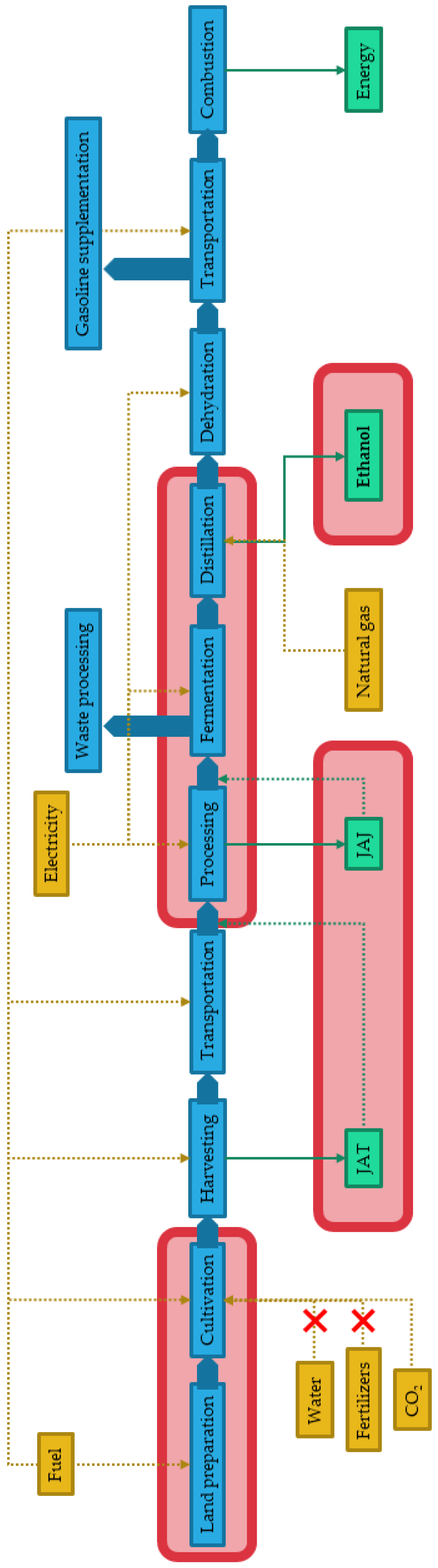
2.1. Bioethanol from Jerusalem Artichoke

Paixão et al. (2018) describes the production of bioethanol using JA as biomass, through a consolidated bioprocessing (CBP) method, which proved to be the best of the tested setups [24]. Plants were cultivated in marginal forest soil without any irrigation (besides precipitation) or fertilizers. Juice was extracted from the tubers to be used for fermentation, by Zygosaccharomyces bailii strain Talf1. A fermentation culture was maintained for 8 days, as the organism used the 130 g/L of fermentable sugars present in the medium to produce ethanol.

Data from all the laboratory-scale processes (juice extraction, juice sterilization and fermentation) was gathered for the modelling of an industrial scenario, in a 20,000 L fermentation tank, agitated by paddles at 200 rpm. This paper will follow the described line of work for a development of an LCA study on the case, considering the maximum ethanol productivity of 3.62 g/L/h (corresponding to a yield of 0.06 L_EtOH/kg_feedstock).

2.2. Life Cycle Assessment

2.2.1. Functional Unit

The functional unit was defined as one liter of produced ethanol (1 L_EtOH ≈ L_EtOH).

2.2.2. System Boundaries

Considering the most approachable and relevant steps for the process and scale-up design, key stages of the ethanol production from JA were selected (Figure 1): land preparation, cultivation of JA tubers, processing of harvested products, fermentation for the production of ethanol, distillation and respective energy inputs and outputs.

2.2.3. Life Cycle Inventory

The Ecoinvent 3.3 (2016) [36] library was used for the LCA study. The Simapro software’s library was used for the electricity mix of Portugal (

Table 3. Electricity mix for Portugal (2016), for the production of 1 kWh.

Input	Value (kWh)
Geothermal	0.008
Hard coal	0.445
Hydro	0.306
Wind	0.241
Compensation for grid losses	0.308
Emissions (gCO2/kWh)	295

) and values not directly measured or calculated by the authors. The CO₂eq intensity for this electricity mix is gCO₂eq/kWh.

Inventory data was considered for a scenario of a 20,000-L industrial fermenter (

Table 4. Inventory for the considered processes of bioethanol production from Jerusalem artichoke.

Process	Item	Value
Land preparation	Area	1.000 ha
	Diesel	0.023 L
Cultivation	Water	0.000 L
	JA tubers yield	39,069.700 kg
Processing	Electricity	1207.000 kWh
	JA juice yield	27,906.930 kg
Fermentation	Electricity	7035.118 kWh
	EtOH yield	2299.050 L
Distillation	Natural gas	0.179 L

). Common industrial use of this kind of equipment was contemplated. Electricity consumption for an agitator paddle working at 200 rpm was considered. A CO₂ absorption of 1.390 kgCO₂/kg_{JA tubers} was considered. The lack of irrigation for cultivation is highlight, as JA can get its water inputs from common rain water (as opposed to other ethanol feedstock) [24].

2.2.4. Impact Assessment

Considering the scope of this work and the impact category to be analyzed, the following LCA methods were used to assess GWP, as they produced results in mass of CO₂eq for a given product assembly process: TRACI 2005 2.1, IPCC GWP 20 years 1.01, ILCD 2011 Midpoint+ 1.07, IMPACT 2002+ 2.12, EDIP 2003 1.05, and CML 2001 2.05 20 years, 100 years and 500 years.

Global warming is considered to be the warming that can be caused by increased emission of GHG from human activities. GWP are used to calculate the potency of GHG (CO₂, CH₄, N₂O) relative to 1 kg of CO₂ at time zero [37].

No allocation or system expansion was performed.

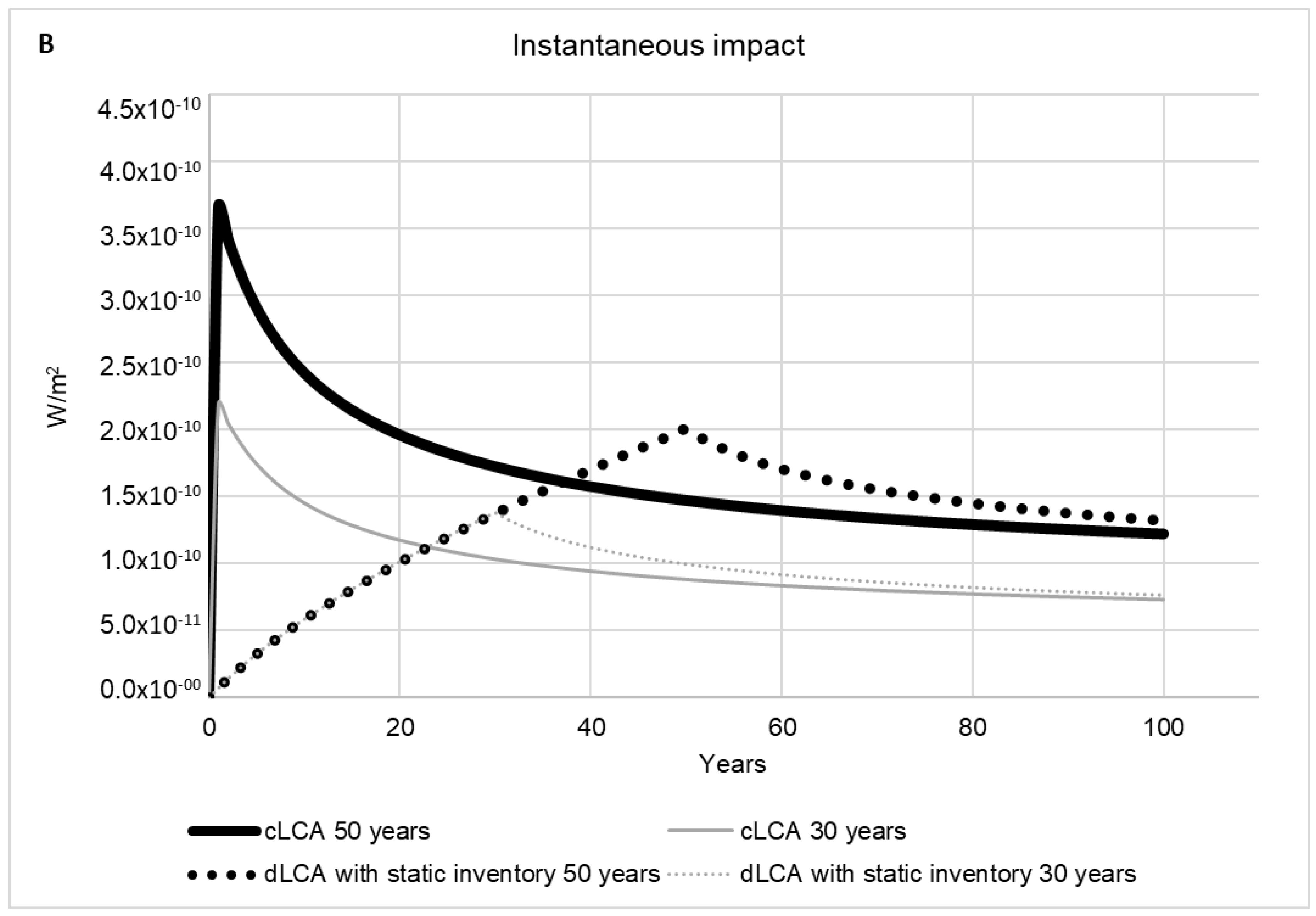
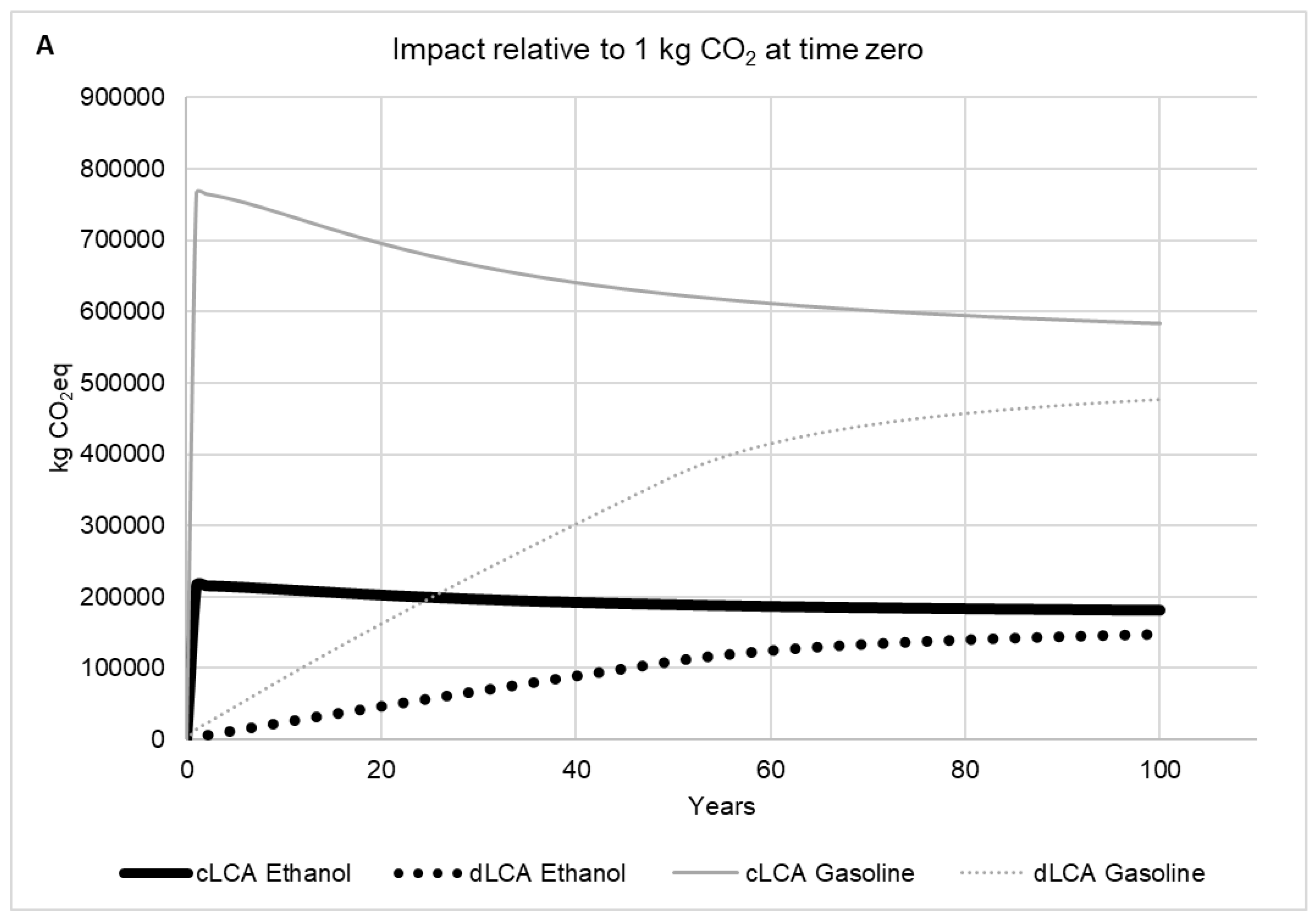
2.2.5. Time Horizon Influence

The IPCC recommends the use of a 100-year time horizon to see the amount of CO₂ that has the same radiative forcing 100 years from time zero. However, 20 years or 500 years could also be used. For example, the impact assessment methodologies CML 2001 have these possible time horizons.

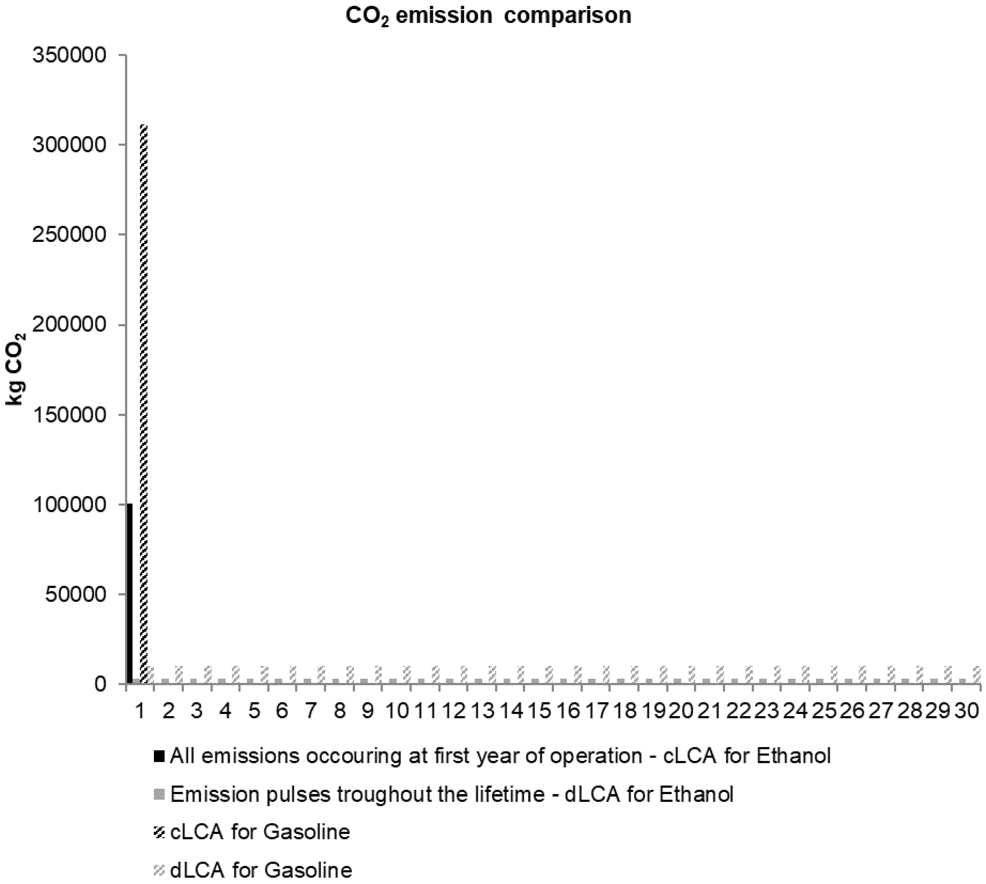
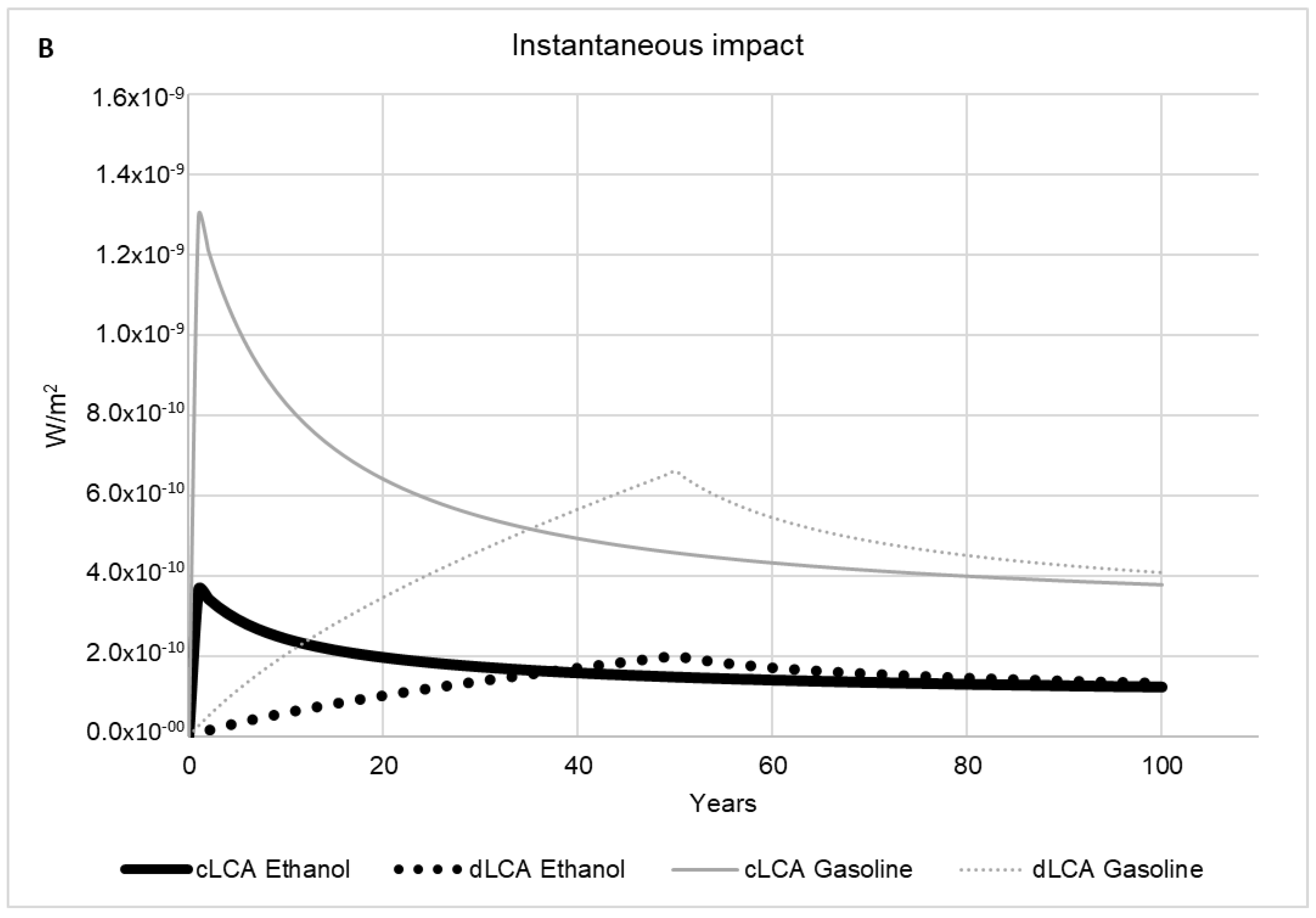
2.2.6. Dynamic LCA versus Conventional LCA

The cLCA as in the case of the reviewed studies, the emissions are assumed to occur in the first year of the factory operation (between 0 and 1 year, see Figure 2), and the reality is that emissions are produced throughout the factory lifetime (dLCA, constant pulse emissions throughout the lifetime).

Each emission pulse follows a lifetime decay due to nature mechanisms throughout time and, therefore, its global warming potential also changes throughout time.

The Bern carbon cycle was used to model the emission pulses decay [38]:

$$C_{C{O}_2}\left(t\right)=a0+{{\displaystyle \sum }}_{i=1}^a{a}_i{e}^{-\frac{t}{\tau i}}$$

(1)

where $a$0 = 0.217, $a$1 = 0.259, $a$2 = 0.338, $a$3 = 0.186, τ1 = 172.9, τ2 = 18.51, τ3 = 1.186.

For CH₄ and N₂O:

$$C_{{\mathrm{CH}}_4 or {\mathrm{N}}_2\mathrm{O}}\left(t\right)=e^{-\frac{t}{\tau i}},$$

(2)

where τCH₄ = 12, τN₂O = 114.

The radiative forcing (RF_x) in W/m²/kg of emission is computed for an atmospheric background CO₂ of 389 ppm: 1.77 × 10⁻¹⁵ W·m⁻²·kg-CO₂⁻¹; 1.1682 × 10⁻¹³ W·m⁻²·kg-CH₄⁻¹ and 3.54 × 10⁻¹³ W·m⁻²·kg-N₂O⁻¹ [39].

A pulse emission (E(t)) has an instantaneous radiative forcing RF given by:

RF (t) [W/m²] = E(t) × RF_x,

(3)

or, considering all emission pulses since time zero, the cumulative radiative forcing, or absolute global warming potential (AGWP) is as follows.

$$\mathrm{AGWP}(\mathrm{t})[\mathrm{W}/{\mathrm{m}}^2]={{\displaystyle \int }}_{t0}^{t}R{F}_x\left(t\right)C_x\left(t\right)dt,$$

(4)

where x stands for the emission CO₂, CH₄ and N₂O.

The AGWP divided by the AGWP of 1 kg CO₂ pulse at time zero stands for the GWP, in a certain time horizon (TH), in CO₂eq, is given by,

$$GWP\left(TH\right)=\frac{{{\displaystyle \int }}_x^{}{{\displaystyle \int }}_{t0}^{t}R{F}_x\left(t\right)C_x\left(t\right)dt}{{{\displaystyle \int }}_{t0}^{t}R{F}_{C{O}_2}·C_x\left(t\right)dt}$$

(5)

An open-source Excel spreadsheet with the above-described model from CIRAIG [40] was used for our calculations.

A scenario of a fermenter producing 10,000 L of bioethanol per year was considered, over a life time of 30 years or 50 years. For the fermenter lifetime, a constant emission per year was GHG emissions were: 3353.733 kg CO₂/year, 7.826 kg CH₄/year, and 0.113 kg N₂O/year.

3. Results and Discussion

Table 5. Inventory for the considered processes of bioethanol production for JA. LCA methods legend—T: TRACI 2005 2.1; IP: IPCC GWP 20 years 1.01; IL: ILCD 2011 Midpoint+ 1.07; IM: IMPACT 2002+ 2.12; E: EDIP 2003 1.05; C20/100/500: CML 2001 2.05 20/100/500 years. Gasoline and ethanol from sugarcane values are correspondent to cradle-to-gate approach, and do not include allocation or transport.

		Value (kg CO2eq/LETOH)
	Method	T	IP	IL	IM	E	C20	C100	C500
	Time horizon	100	20	100	100	100	20	100	500
	Country	USA	n/a	n/a	Switzerland	Denmark	Netherlands
Processes	Ethanol from JA (this study)
	Land preparation and cultivation	0.0456	0.0469	0.0456	0.1390	0.1430	0.0466	0.0458	0.0452
	Processing	0.1130	0.1300	0.1130	0.1120	0.1160	0.1230	0.1130	0.1080
	Fermentation	0.2010	0.2310	0.2010	0.1190	0.2070	0.2190	0.2000	0.1920
	Distillation	2.56 × 10−8	4.90 × 10−8	2.56 × 10−8	1.88 × 10−6	2.56 × 10−8	4.01 × 10−8	2.48 × 10−8	1.85 × 10−8
	Total	0.3600	0.4800	0.3600	0.4490	0.4660	0.3890	0.3590	0.3450
	Gasoline [32,35]	1.154
	Ethanol from sugarcane [32,35]	0.75

shows the emissions of CO₂eq per liter of bioethanol produced by the fermentation process described above, as calculated by different LCA impact assessment methodologies, and compares them with the standard gasoline and ethanol production indicated by JRC [33].

In all cases, ethanol production using JA appears to have slightly higher emissions than “standard” 1G ethanol from sugarcane. The presented value from JRC [33] considers sugarcane and ethanol production (and excludes transportation), but these two main processes do not discriminate sub-processes such as harvesting or distillation, which might lead to different emission results. Conflicting or disparate results in LCA studies are often attributed to the use of functional units, system boundaries, and/or methods as well as the lack of information and data that is published [40]. In fact, even when considering the same processes, the different selected methods ended up giving different emission results. As shown in Table 5, some methods have different time horizons and were made in different countries, and one might infer that that could have an influence on the genesis of the method.

The different values for the same metric GWP, 100 years TH, in CO₂eq, have to do with different considerations, for example, the impact assessment method IM considers CO emission oxidation to CO₂ and E, and in addition to CO oxidation considers NOx conversion to N₂O, and therefore has higher CO₂eq values (difference for minimum up to 30%). The influence of the TH can be observed in the C impact assessment methodology, producing a range 0.345–0.389 kg CO₂eq/L_ETOH (difference for minimum up to 13%).

Figure 3 addresses the factory placement issue, different locations/countries mean different electricity mixes. Different countries, with different political and economic landscapes as well as different natural and technological resources, have different ways of generating and managing energy. Using the TRACI method (which, along with ILCD, resulted in the lowest GHG emission value) for impact calculation, the process was kept the same, but electricity input was changed according to the electricity mix of different countries (from the Ecoinvent 3.3 library), affecting the “processing” and “fermentation” steps of the production chain (according to the electricity needs of these states, see Table 4). Portugal ranked third among the other three countries selected for this example. The differences can be mostly attributed to the use of renewable and nuclear energies. These types of energies are considered to be of null or low CO₂eq emissions, and their use in France and Brazil is evidently higher than in Portugal and India, which for their part have a higher reliance on coal and oil [1].

As can be seen, the electricity mix alone can cause a range of results from 0.1 to 0.85 kgCO₂eq/L_EtOH (deviation from minimum up to 750%).

The chronological time at which the study is carried out can also be considered, as they might use different IPCC assessment reports (AR) for GWP relative to CO₂eq values. For example, the carbon footprint for the 100-year time horizon for methane was, as in the IPCC’s AR2 (1996), 21, but in AR5 (2013) it rose to 28, meaning that the release of 1 kg of this gas went from being equivalent to 21 to 28 kgCO₂, in 17 years [43]. However, when GHG values from different ARs are considered for the production of ethanol studied in this work, the differences are not so relevant (Figure 4).

As can be seen, the use of different IPCC assessment reports does not have a significant impact in CO₂eq values (deviation from the minimum less than 3%). This is due to the fact that GHG emissions from fossil origin considered in the inventory of the work are mainly composed of CO₂, in a much higher percentage than methane or nitrous oxides. As 1 kgCO₂ is always 1 kgCO₂eq, the time at which the study was made is not relevant, and the same can eventually be applied to comparisons with other studies. This type of result is indicative of the difficulty to compare different studies and correlate year-zero emissions to long term GHG impact and interested readers and decision-makers must be aware of the temporal evolution of assumptions. Nevertheless, time can still be taken into account in LCA studies. Emissions are usually considered in a single aggregate emission. There is a lack of information about emissions from processes during the time at which they occur, and this type of study relies on restricted steady-state models, but this decreases accuracy and comes as a great limitation. Considering the instantaneous release of a large amount of GHG does not have the same impact as the release of the same amount at a small rate over several years [44]. Figure 5A shows differences of impacts relative to 1 kgCO₂ at time zero, considering instantaneous (solid line) and dynamic (dotted line). The dynamic impact, at the 30-year mark, is of −42.2% compared to the instantaneous scenario, softening to a value of −10.9% at 100 years. Figure 5B shows that the instantaneous impact, at the same mark, is 33.0% when considering emissions over 30 years versus all the emissions being theoretically released in the first year, converging to a 4.1% at 100 years. The difference between these two time horizons is quite relevant and is an example of the relevance and need for carefully analyzing temporal factors in industry scenarios. In LCA studies, not considering the temporal profile of the subject can lead to an underestimation of impacts of GHG emissions, which can then result in different decision-making processes.

The lifetime of the factory also has an influence on the CO₂eq results, the longer the lifetime, the higher the impacts. The 20 years’ difference between cLCA and dLCA is 61% and for the 100 years difference between dLCA and cLCA is of −10%. Therefore, the deviation from the minimum value at 20 years is up to 159% and 12% for 100 years. The same values for 50 years of operation are 332% and 23%, respectively. The cLCA having always the higher values, which means researchers are systematically overestimation the carbon footprints.

Figure 6 shows the influence of future productivity improvements due to genetic modifications [45,46,47,48,49]. Results obtained under Simapro software analysis using the TRACI method were similar to the ones obtained previously [24], no biogenic, no land use, no allocation and cradle-to-gate borders with no transportation.

As can be seen, future productivity improvements can cause a range from 0.05 up to almost 0.45 kgCO₂eq/LEtOH, with a possible reduction of emissions of around 800%.

Finally, besides calculating the carbon footprint of a biomass-to-bioethanol pathway, we also compare this with an equivalent fossil biomass-to-gasoline pathway, with the same assumptions (in CO₂eq/L_EtOHeq, based on LHV ratio). Of course, a refinery is a multiproduct system, and our case study is a single product factory, so the comparison is unfair from the beginning. Nevertheless, a comparison of systems on cLCA versus dLCA view is depicted in Figure 7.

For impact relative to 1 kg CO₂ at time zero of the ethanol equivalent scenario, at 20- and 100-year time horizons, a difference of −77% and −18% can be seen between dLCA and cLCA, respectively. As for instantaneous impact, the same time horizons present differences of −46% and 8%. As previously noted, high cLCA values can lead to an overestimation of impacts; however, the biomass-to-ethanol approach is clearly less impactful than oil-to-ethanol.

4. Conclusions

This paper seeks to quantify impacts of methodological choices on CO₂eq emissions of a biomass-to-ethanol pathway so future studies include as much information as possible. From the non-extensive literature review we found, in terms of deviations from the minimum values the following influences:

Allocation up to 83%, land use up to 271%, and biogenic up to 240%.

From our study we found that the same deviations were as follows, considering the different topics analyzed:

Impact assessment methods up to 30%, location of the factory (countries’ electricity mix) up to 750%, IPCC assessment reports up to 3%, time horizon (20 or 100 years) up to 13%, factory operational lifetime up to 108%, and productivity up to 800%.

Therefore, to make an informed decision, we argue that every carbon footprint study should have, besides the uncertainty due to inventory data, a sensitivity analysis for other parameters, mainly those that are foreseen to have a higher impact based on our study: factory location (or future electricity mix projections, or own local electricity production), land use issues, no allocation and allocation, and dynamic evaluation. We also argue that if the carbon footprint of the pathway is not the aim, the comparison with other system should be made by using the same premises, i.e., same methodological options. The comparison between the biomass-to-ethanol and oil-to-ethanol equivalent approach clearly showed the higher impacts of the later, with differences up to 222% between the cLCA of both approaches, and 209% for dLCA, at 100 years, easily distinguishing the most environmentally friendly scenario. Of course, a refinery is a multiproduct system and our case study a single product factory, so the comparison is unfair from the beginning.

It is very important for the decision maker to have the awareness that a carbon footprint is not a hard number and always has a huge range attached to a mean value. The higher the operational factory time the higher the differences between conventional and dynamic GWP metric.

References

1. U.S. Energy Information Administration—U.S. Department of Energy. EIA International Energy Outlook 2009; Technical Report for Energy Information Administration: Washington, DC, USA, May 2009.
2. Axelsson, L.; Franzén, M.; Ostwald, M.; Berndes, G.; Lakshmi, G.; Ravindranath, N.H. Perspective: Jatropha cultivation in southern India: Assessing farmers’ experiences. Biofuels Bioprod. Biorefin. 2012, 6, 246–256. [Google Scholar] [CrossRef]
3. Morales, M.; Quintero, J.; Conejeros, R.; Aroca, G. Life cycle assessment of lignocellulosic bioethanol: Environmental impacts and energy balance. Renew. Sustain. Energy Rev. 2015, 42, 1349–1361. [Google Scholar] [CrossRef]
4. Giuntoli, J. Final Recast Renewable Energy Directive for 2021–2030 in the European Union; Report for International Council on Clean Transportation: Washington, DC, USA, July 2018. [Google Scholar]
5. International Energy Agency. IEA Energy Technology Essentials Biofuel Production; Technical Report for International Energy Agency: Paris, France, 24 April 2007; pp. 1–4. [Google Scholar]
6. Heywood, J. Internal Combustion Engine Fundamentals; McGraw-Hill Education: New York, NY, USA, 16 May 1988. [Google Scholar]
7. Combustion of Fuels—Carbon Dioxide Emission. Available online: https://www.engineeringtoolbox.com/co2-emission-fuels-d_1085.html (accessed on 13 June 2019).
8. Sendelius, J. Steam Pretreatment Optimisation for Sugarcane Bagasse in Bioethanol Production. Master’s Thesis, Lund University, Scania, Sweden, January 2005. [Google Scholar]
9. Quintero, J.A.; Montoya, M.I.; Sánchez, O.J.; Giraldo, O.H.; Cardona, C.A. Fuel ethanol production from sugarcane and corn: Comparative analysis for a Colombian case. Energy 2008, 33, 385–399. [Google Scholar] [CrossRef]
10. Cardona, C.A.; Sánchez, Ó.J. Fuel ethanol production: Process design trends and integration opportunities. Bioresour. Technol. 2007, 98, 2415–2457. [Google Scholar] [CrossRef]
11. Cheng, K.K.; Cai, B.Y.; Zhang, J.A.; Ling, H.Z.; Zhou, Y.J.; Ge, J.P.; Xu, J.M. Sugarcane bagasse hemicellulose hydrolysate for ethanol production by acid recovery process. Biochem. Eng. J. 2008, 38, 105–109. [Google Scholar] [CrossRef]
12. Cardona, C.A.; Quintero, J.A.; Paz, I.C. Production of bioethanol from sugarcane bagasse: Status and perspectives. Bioresour. Technol. 2010, 101, 4754–4766. [Google Scholar] [CrossRef]
13. McMillan, J.D. Bioethanol production: Status and prospects. Renew. Energy 1997, 10, 295–302. [Google Scholar] [CrossRef]
14. Slininger, P.J.; Shea-Andersh, M.A.; Thompson, S.R.; Dien, B.S.; Kurtzman, C.P.; Balan, V.; Balan, V.; Sousa, L.D.C.; Uppuqundla, N.; Dale, B.E.; et al. Evolved strains of Scheffersomyces stipitis achieving high ethanol productivity on acid- and base-pretreated biomass hydrolyzate at high solids loading. Biotechnol. Biofuels 2015, 8, 1–27. [Google Scholar] [CrossRef]
15. Demeke, M.M.; Dumortier, F.; Li, Y.; Broeckx, T.; Foulquié-Moreno, M.R.; Thevelein, J.M. Combining inhibitor tolerance and D-xylose fermentation in industrial Saccharomyces cerevisiae for efficient lignocellulose-based bioethanol production. Biotechnol. Biofuels 2013, 6, 1–17. [Google Scholar] [CrossRef]
16. Duda, M.; Shaw, J.S. Life Cycle Assessment. Soc. Sci. Public Policy 1997, 35, 38–43. [Google Scholar] [CrossRef]
17. Ekvall, T.; Finnveden, G. Allocation in ISO 14041—A critical review. J. Clean. Prod. 2001, 9, 197–208. [Google Scholar] [CrossRef]
18. Finnveden, G.; Hauschild, M.Z.; Ekvall, T.; Guinée, J.; Heijungs, R.; Hellweg, S.; Koehler, A.; Pennington, D.; Suh, S. Recent developments in Life Cycle Assessment. J. Environ. Manag. 2009, 91, 1–21. [Google Scholar] [CrossRef]
19. Ometto, A.R.; Hauschild, M.Z.; Roma, W.N.L. Lifecycle assessment of fuel ethanol from sugarcane in Brazil. Int. J. Life Cycle Assess. 2009, 14, 236–247. [Google Scholar] [CrossRef]
20. Luo, L.; Voet, E.V.D.; Huppes, G. An energy analysis of ethanol from cellulosic feedstock-Corn stover. Renew. Sustain. Energy Rev. 2009, 13, 2003–2011. [Google Scholar] [CrossRef]
21. Kadam, K.L. Environmental Life Cycle Implications of Using Bagasse-Derived Ethanol as a Gasoline Oxygenate in Mumbai (Bombay); NREL/TP-580-28705; Technical Report for National Renewable Energy Laboratory: Lakewood, CO, USA, November 2000.
22. Spatari, S.; Zhang, Y.; Maclean, H.L. Life Cycle Assessment of Switchgrass- and Corn Automobiles. Environ. Sci. Technol. 2005, 39, 9750–9758. [Google Scholar] [CrossRef]
23. Muñoz, I.; Flury, K.; Jungbluth, N.; Rigarlsford, G.; I Canals, L.M.; King, H. Life cycle assessment of bio-based ethanol produced from different agricultural feedstocks. Int. J. Life Cycle Assess. 2014, 19, 109–119. [Google Scholar] [CrossRef]
24. Paixão, S.M.; Alves, L.; Pacheco, R.; Silva, C.M. Evaluation of Jerusalem artichoke as a sustainable energy crop to bioethanol: energy and CO2eq emissions modeling for an industrial scenario. Energy 2018, 150, 468–481. [Google Scholar] [CrossRef]
25. Negro, M.J.; Ballesteros, I.; Manzanares, P.; Oliva, J.M.; Saez, F.; Ballesteros, M. Inulin-containing biomass for ethanol production. Appl. Biochem. Biotechnol. 2006, 132, 922–932. [Google Scholar] [CrossRef]
26. Gengmao, Z.; Mehta, S.K.; Zhaopu, L. Use of saline aquaculture wastewater to irrigate salt-tolerant Jerusalem artichoke and sunflower in semiarid coastal zones of China. Agric. Water Manag. 2010, 97, 1987–1993. [Google Scholar] [CrossRef]
27. Zhang, T.; Chi, Z.; Zhao, C.H.; Chi, Z.M.; Gong, F. Bioethanol production from hydrolysates of inulin and the tuber meal of Jerusalem artichoke by Saccharomyces sp. W0. Bioresour. Technol. 2010, 101, 8166–8170. [Google Scholar] [CrossRef]
28. Hu, N.; Yuan, B.; Sun, J.; Wang, S.A.; Li, F.L. Thermotolerant Kluyveromyces marxianus and Saccharomyces cerevisiae strains representing potentials for bioethanol production from Jerusalem artichoke by consolidated bioprocessing. Appl. Microbiol. Biotechnol. 2012, 95, 1359–1368. [Google Scholar] [CrossRef]
29. Kim, S.; Park, J.M.; Kim, C.H. Ethanol production using whole plant biomass of jerusalem artichoke by Kluyveromyces marxianus CBS1555. Appl. Biochem. Biotechnol. 2013, 169, 1531–1545. [Google Scholar] [CrossRef]
30. Macedo, I.C.; Seabra, J.E.A.; Silva, J.E.A.R. Greenhouse gases emissions in the production and use of ethanol from sugarcane in Brazil: The 2005/2006 averages and a prediction for 2020. Biomass Bioenergy 2008, 32, 582–595. [Google Scholar] [CrossRef]
31. Seabra, J.E.A.; Macedo, I.C.; Chum, H.L.; Faroni, C.E.; Sarto, C.A. Life cycle assessment of Brazilian sugarcane products: GHG emissions and energy use. Biofuels Bioprod. Biorefin. 2011. [Google Scholar] [CrossRef]
32. Tsiropoulos, I.; Faaij, A.P.C.; Seabra, J.E.A.; Lundquist, L.; Schenker, U.; Briois, J.F.; Patel, M.K. Life cycle assessment of sugarcane ethanol production in India in comparison to Brazil. Int. J. Life Cycle Assess. 2014, 19, 1049–1067. [Google Scholar] [CrossRef]
33. Edwards, R.; Lariv_e, J.-F.; Rickeard, D.; Weindorf, W. Report Well-to-Tank Report Appendix 4-Version4a: Description, Results and Input Data per Pathway, April 2014, JRC Technical Reports—Report EUR 26237 EN, JEC-Joint Research Centre-EUCAR-CONCAWE Collaboration, 2014, 1–12. Available online: http://iet.jrc.ec.europa.eu/about-jec/downloads (accessed on 25 April 2019).
34. Neeft, J.; Buck, S.; Gerlagh, T.; Gapnepain, B.; Bacovsky, D.; Ludwiczek, N.; Lavelle, P.; Thonier, G.; Lechón, Y.; Lago, C. Biograce—Harmonised Calculations of Biofuel Greenhouse Gas Emissions in Europe; Technical Report for Intelligent Energy Europe: Brussels, Belgium, June 2019. [Google Scholar]
35. Greenhouse Gases, Regulated Emissions and Energy Use in Transportation (GREET). Available online: https://greet.es.anl.gov/ (accessed on 2 March 2019).
36. The Ecoinvent Database Version 3 (Part I): Overview and Methodology. Available online: http://link.springer.com/10.1007/s11367-016-1087-8 (accessed on 20 November 2018).
37. Bare, J.C. The tool for the reduction and assessment of chemical and other environmental impacts 2.0. J. Ind. Ecol. 2011, 13, 687–696. [Google Scholar] [CrossRef]
38. Shimako, A. Contribution to the Development of a Dynamic Life Cycle Assessment Method. Ph.D. Thesis, Institut National des Sciences Appliquées de Toulouse, Toulouse, France, 2017. [Google Scholar]
39. Joos, F.; Roth, R.; Fuglestvedt, J.S.; Peters, G.P.; Enting, I.G.; Bloh, W.V.; Brovkin, V.; Burke, E.J.; Eby, M.; Edwards, N.R.; et al. Carbon dioxide and climate impulse response functions for the computation of greenhouse gas metrics: A multi-model analysis. Atmos. Chem. Phys. 2013, 13, 2793–2825. [Google Scholar] [CrossRef]
40. Levasseur, A.; Lesage, P.; Margni, M.; Deschênes, L.; Samson, R. Considering time in LCA: dynamic LCA and its application to global warming impact assessments. Environ. Sci. Technol. 2010, 44, 3169–3174. [Google Scholar] [CrossRef]
41. Moro, A.; Lonza, L. Electricity carbon intensity in European Member States: Impacts on GHG emissions of electric vehicles. Transp. Res. Part D: Transp. Environ. 2018, 64, 5–14. [Google Scholar] [CrossRef]
42. Climate Transparency Organization. G20 Brown to Green Report 2018; Climate Transparency, c/o Humboldt-Viadrina Governance Platform: Berlin, Germany, 2018. [Google Scholar]
43. Silva, C.; Pacheco, R.; Arcentales, D.; Santos, F. Sustainability of sugarcane for energy purposes—Chapter 3. In Sugarcane Biorefinery, Technology and Perspectives; Academic Press: Cambridge, MA, USA, 2019; ISBN 978-0-12-814236-3. (in press) [Google Scholar]
44. Borrion, A.L.; McManus, M.C.; Hammond, G.P. Environmental life cycle assessment of lignocellulosic conversion to ethanol: A review. Renew. Sustain. Energy Rev. 2012, 16, 4638–4650. [Google Scholar] [CrossRef]
45. Kosugi, A.; Kondo, A.; Ueda, M.; Murata, Y.; Vaithanomsat, P.; Thanapase, W.; Arai, T.; Mori, Y. Production of ethanol from cassava pulp via fermentation with a surface-engineered yeast strain displaying glucoamylase. Renew. Energy 2009, 34, 1354–1358. [Google Scholar] [CrossRef]
46. Yamada, R.; Tanaka, T.; Ogino, C.; Fukuda, H.; Kondo, A. Novel strategy for yeast construction using δ-integration and cell fusion to efficiently produce ethanol from raw starch. Appl. Microbiol. Biotechnol. 2010, 85, 1491–1498. [Google Scholar] [CrossRef]
47. Aydemir, E. Genetic Modifications of Saccharomyces cerevisiae for Ethanol Production from Starch Fermentation: A Review. J. Bioprocess. Biotech. 2014. [Google Scholar] [CrossRef]
48. Shigechi, H.; Uyama, K.; Fujita, Y.; Matsumoto, T.; Ueda, M.; Tanaka, A.; Fukuda, H.; Kondo, A. Efficient ethanol production from starch through development of novel flocculent yeast strains displaying glucoamylase and co-displaying or secreting α-amylase. J. Mol. Catal. B Enzym. 2002, 17, 179–187. [Google Scholar] [CrossRef]
49. Ramachandran, N.; Joubert, L.; Gundlapalli, S.B.; Otero, R.R.C.; Pretorius, I.S. The effect of flocculation on the efficiency of raw-starch fermentation by Saccharomyces cerevisiae producing the Lipomyces kononenkoae LKA1-encoded α-amylase. Ann. Microbiol. 2008, 58, 99–108. [Google Scholar] [CrossRef]
Figure 1. Process chain for the production of bioethanol from JA. Blue boxes: main processes; Yellow boxes: inputs; Green boxes: outputs. All processes were considered to emit CO2eq. System boundaries include the red highlighted processes and respective inputs and outputs. (JAT: JA tubers; JAJ: JA juice).
Energies 12 02535 g001
Figure 2. Example of the difference in conventional CO2 emissions and actual emissions during a factory lifetime. Comparison between our case study for ethanol [24] and gasoline, without allocation, in a cradle-to-gate approach [33], for a 30-year operation lifetime.
Energies 12 02535 g002
Figure 3. Comparison of emissions for the production of 1 LEtOH, considering electricity mixes from different countries and CO2 intensity (CO2/kWh) (R: renewable energies; N: nuclear energy) [41,42].
Energies 12 02535 g003
Figure 4. Comparison of GWP, using different values for CO2eq, considered in the referenced IPCC ARs, for 100 years.
Energies 12 02535 g004
Figure 5. (A) Comparison of GW impacts relative to 1 kg of CO2 at time zero between conventional and dynamic scenarios of GHG emissions (see Equation (5)). (B) Comparison of GW instantaneous impacts between conventional and dynamic scenarios of GHG emissions (see Equation (4)). Values considered for a scenario of an industrial facility working for 30 and 50 years.
Energies 12 02535 g005aEnergies 12 02535 g005b
Figure 6. Relationship between productivity and emissions from different simulated scenarios, considering possible genetic modification of yeast strains. Results for the present study only include TRACI values (see Table 5).
Energies 12 02535 g006
Figure 7. Relationship between biomass-to-ethanol and crude oil-to-ethanol equivalent (gasoline). (A) Comparison of GW impacts relative to 1 kg of CO2 at time zero between conventional and dynamic scenarios of GHG emissions (see Equation (5)). (B) Comparison of GW instantaneous impacts between conventional and dynamic scenarios of GHG emissions (see Equation (4)).
Energies 12 02535 g007aEnergies 12 02535 g007b