Abstract
Germany has experienced rapid growth in onshore wind capacities over the past two decades. Substantial capacities of offshore wind turbines have been added since 2013. On a local, highly-resolved level, this analysis evaluated if differences in wind speed forecast errors exist for offshore and onshore locations regarding magnitude and variation. A model based on the Extra Trees algorithm is proposed and found to be a viable method to transform local wind speeds and capacities into aggregated wind energy feed-in. This model was used to analyze if offshore and onshore wind power expansion lead to different distributions of day-ahead wind energy forecast errors in Germany. The Extra Trees model results indicate that offshore wind capacity expansion entails an energy forecast error distribution with more frequent medium to high deviations, stemming from larger and more variable wind speed deviations of offshore locations combined with greater geographical concentration of offshore wind turbines and their exposure to high-wind oceanic conditions. The energy forecast error distribution of onshore expansion, however, shows heavier tails and consequently more frequent extreme deviations. The analysis suggests that this can be rooted in the simultaneous over- or underestimation of wind speeds at many onshore locations.
1. Introduction
Germany has seen rising onshore wind capacities in the past two decades, with a total installed capacity of around 56 GW at the end of 2018. At the same time, ca. 5.6 GW of offshore wind parks were installed, with substantial capacities starting to be added in 2013. These large capacities make substantial contributions to the renewable energy generation. Large, additional wind offshore parks are supposed to be completed or fully commissioned in 2019, e.g., Arkona (385 MW, commissioned in April), Borkum Riffgrund II (450 MW, commercial commissioning completed in June), Deutsche Bucht (269 MW), Hohe See (497 MW), Merkur (396 MW, already partly commissioned) and Trianel Borkum II (200 MW). Until 2025, the total offshore wind capacity in Germany will reach almost 12 GW. The capacities are obtained from a self-compiled dataset, with information on planned offshore power plants [1,2,3,4,5,6,7,8,9,10,11,12,13,14,15,16,17,18].
Wind energy forecasts are subjected to uncertainties due to errors in wind speed predictions. Wind energy is characterized by variability and limited predictability. Additionally, it affects the power system at all hours of the day and does not necessarily coincide with load. This affects day-ahead decisions of operators of wind turbines and conventional power plants, e.g., unit commitment of conventional power plants, taking into account forecasts for renewable energy generation, available at the time of decision. The uncertainties also influence the operation of power systems with the challenge of maximizing the capability of integrating fluctuating wind energy.
With increasingly prevalent offshore wind energy capacities, differences between onshore and offshore locations become more important for energy systems. Offshore wind capacities are geographically concentrated to a higher degree due to large wind turbines and large-scale wind parks. Generally, oceanic conditions and large hub heights result in high wind speeds for offshore wind turbines. Because of the cubic relation between wind speed and power output, wind speed forecast errors cause greater deviations in output at medium to high wind speeds, compared with low wind speeds. This, in turn, could mean that offshore wind speed deviations have a greater effect on wind energy forecast errors, even when compared to onshore wind speed deviations of equal magnitude.
With particular regard to the planned expansion of offshore wind capacities, this study analyzed actual and forecast wind speeds at a high geographical resolution from the ECMWF database. The resulting deviations were used to evaluate: (1) if differences exist in wind speed forecast errors for onshore and offshore locations; and (2) if these possible differences, combined with greater concentration and higher wind speeds of offshore wind capacities, lead to higher deviations in overall wind energy forecasts.
The first question is answered with a statistical analysis of local wind speed forecast errors. For the second question, an Extra Trees model is developed to transform wind speeds into aggregated forecast and actual wind energy amounts based on different onshore and offshore wind capacities. The resulting deviation distributions were used to identify differences between the expansion of onshore and offshore wind energy capacities. The proposed approach is a top-down estimate, decoupled from technical information on wind energy turbines.
The remainder of this paper is structured as follows. Section 2 gives a brief overview of the literature dealing with wind power uncertainties. Section 3 describes the data sources used for this analysis. A statistical analysis of local wind speed data that was conducted and evaluated is presented in Section 4. This is followed by the description and evaluation of the Extra Trees model in Section 5. Section 6 concludes this analysis and highlights key findings.
2. Literature Review
Large-scale wind generation poses several challenges for power system operation caused by the limited predictability and variability of wind energy and its intermittent nature [19,20,21]. These challenges can be amplified due to the negative correlation of wind power and load [22], which stands in contrast to other sources of variable renewable energy, especially photovoltaics.
A large field of research deals with unit commitment under wind energy uncertainties [20,21,22,23,24,25,26,27,28,29,30]. Unit commitment decisions become more complex due to the priority feed-in of wind power in most electricity markets [31]. Increasing shares of fluctuating wind power can translate into less certain quantification of the provision of system reserve as well as an increased need for regulating and reserve power [23,25,32].
Further challenges can be frequency control issues, planning of the transmission network and extra requirements for energy reserves [25]. Uncertainties, which stem from rising penetration of variable energy sources, can lead to unpredicted power balancing problems, posing a risk for system reliability. Unforeseen mismatches of load forecast and wind forecast errors can lead to additional system costs, requiring additional balancing services. This necessitates information on the probability and magnitude of the described problems [26].
These challenges need to be adequately taken into account to allow wind energy to substitute conventionally generated electricity. This imposes high demands for balancing services and intraday trading [33,34]. Naturally, uncertain wind power availability does not only affect the operators of transmission and distribution systems and conventional dispatchable power plants but also the operators of wind farms, whose certain day-ahead production commitment is impaired [35,36,37,38]. It is important to mention that the probability distribution of wind speeds affects not only the operation but also the planning and design of wind turbines and wind parks, along with factors such as altitude, tower height and turbines interactions (e.g., wake effects) [39]. Furthermore, wind energy forecasts substantially affect the price distribution [40]. Variable wind power negatively correlates with the price level and increases price volatility [41].
The above-described challenges and their economic significance for the power system stress the importance of accurate wind speed and wind energy forecasts for the dispatch schedules in the day-ahead electricity market [42], for which there is a wide array forecasting methods [31,39,42,43,44,45,46,47]. A thorough overview of recent advances in statistical wind energy forecasting is provided in [48]. The power system benefits from more accurate wind energy forecasts, as they lead to savings in total system costs, especially for deterministic scheduling, lower levels of wind curtailment and decreased dispatch of flexible conventional power plants [31].
The fast expansion of offshore wind energy capacities, not only in Germany, will likely continue in the future, which makes offshore wind speed forecasts increasingly important. The expansion is owed to greater public support for offshore wind parks [49], the scarcity of suitable, remaining onshore wind locations and technological advances and falling technology costs [50,51]. Offshore wind turbines are more centralized and, on average, exposed to higher wind speeds (see discussion in Section 4.1), leading to the possibility that offshore wind speed deviations have a greater effect on wind energy forecast errors. While the accuracy of wind energy forecasts affects the short-term market behavior of market participants and operational costs of power systems, long-term economic effects of added wind power capacities have to be anticipated and quantified as well.
To the best knowledge of the authors, no analysis exists that evaluates the effect of wind speed forecast errors on the overall wind energy forecasts of Germany, separately for onshore and offshore locations. Consequently, the analysis presented here sought to answer three research questions:
- Do deviations of actual wind speeds from forecast values differ between offshore and onshore locations in terms of magnitude, variation and extreme values?
- How are offshore and onshore wind speed deviations distributed when taking into account the “importance” of locations, i.e., installed capacities?
- Does offshore wind capacity expansion introduce more uncertainty into aggregated wind energy forecasts than onshore wind capacity expansion?
3. Data Description
Note that this analysis contains modified Copernicus Atmosphere Monitoring Service Information and modified Copernicus Climate Change Service Information (2016–2018). Neither the European Commission nor European Centre for Medium-Range Weather Forecasts (ECMWF) is responsible for any use that may be made of the information it contains.
The data for this analysis were retrieved from the ECMWF. It contains publicly available datasets for wind speed forecast and actual values. The data can be obtained at a resolution of 0.125 longitude by 0.125 latitude, roughly equal to a 8 km-by-13 km grid in Germany. This allows for a highly resolved representation of wind speed differences, not only within Germany but also offshore. For the analysis, locations within latitudes of 47–55.5 and longitudes of 5.5–15.5 were obtained, resulting in a total of 5589 geographical points.
The forecast wind speeds were taken from the CAMS (Copernicus Atmosphere Monitoring Service) Near-real-time dataset [52]. Points in time, at which forecasts are made, are 0:00 and 12:00, up to 120 h ahead. The time of 12:00 was of greatest interest for this analysis because it is closest to the clearing of the day-ahead market. For the following day, nine point forecasts are available, starting at 0:00 of the subsequent day (twelve hours ahead) until 24:00 (36 h ahead) in 3-h intervals (see Figure 1). The wind speed forecasts were made for a height of 10 m above ground. To retrieve hourly forecasts, the values in between the point forecasts were linearly interpolated, which means forecasts were available for t, , , etc., and interpolation was done for , , etc., using the “nearest” t and forecast values. All nine available point forecasts were needed, including the forecast for 24:00 to correctly estimate values for 22:00 and 23:00. After the interpolated values were estimated, the forecast value for 24:00 was deleted and replaced by the 0:00-forecast of the subsequent day. Interpolation introduces the possibility of incorrectly representing large short-term wind speed changes. This issue is addressed in Section 4.1.
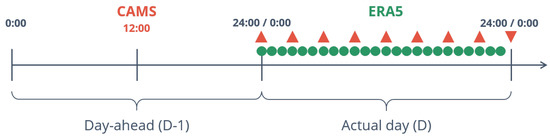
Figure 1.
Displayed is the time line of CAMS forecasts made at 12:00 on the day-ahead and ERA5 actual values. Depicted are nine forecast values (red triangles) and the 24 actual values for the next day (green dots). Note that the forecast for 24:00 (upside-down triangle) was only used for creating interpolated values for 22:00 and 23:00 and subsequently removed. Source: Own diagram.
For the actual values, time series from the ERA5 (5th generation of ECMWF Reanalysis) dataset [53] were retrieved. Here, values for every hour exist. The reanalysis values are available for heights of 10 m and 100 m, which allows for retrieving location-specific roughness values, as discussed in Section 4.
For both the CAMS and ERA5 datasets, monthly datasets from 01 July to 30 November 2016 and 01 February 2017 to 30 September 2018 were retrieved. Forecasts before July 2016 were unavailable at the time of analysis. December 2016 was unavailable as well and January 2017 was an incomplete dataset. Thus, two datasets (01 July to 30 November 2016 and 01 February 2017 to 30 September 2018) with subsequent, uninterrupted time series were used. In total, data for 25 months are available, with a total of 18,240 h. To evaluate forecast errors of wind speeds, the time shift between forecast dataset and actual dataset has to be taken into account. For instance, the first time stamp of the September forecast dataset represents 02 September, 0:00, and the last entry is 01 October, 24:00. For both datasets: (1) the first 24 entries of the actual wind speed values had to be removed due to missing forecast values; and (2) the last 24 entries of the forecast values had to be removed due to missing actual values. This left 18,192 hourly values of forecast and actual wind speeds for each grid.
Finally, the analysis requires geographical locations of the installed onshore and offshore wind turbines. The onshore capacities were retrieved from online wind turbine databases of the federal state offices, agencies and ministries of Germany [1,2,3,4,5,6,7,8,9,10,11,12,13,14,15,16]. The offshore capacities and locations were obtained from The Wind Power and 4C Offshore [17,18]. Subsequently, each individual turbine was assigned to the nearest geographical location of the available grid of the wind speed dataset. This allows for an aggregation of capacities for each location. The resulting assigned capacities are displayed in Figure 2. It clearly shows the high density of wind turbines in the northwest and center of Germany. However, onshore capacities are still more spatially spread out than offshore capacities that show high geographical concentration.
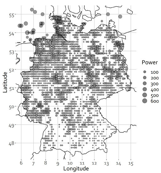
Figure 2.
Capacities assigned to geographical points of the 0.125-by-0.125grid. Source: Own diagram.
4. Data Analysis
The overarching goal of this analysis was to evaluate the effect of increasing offshore wind capacities on the day-ahead forecast errors of aggregated wind energy. To approach this question, a descriptive data analysis preceded the development of the model. Therefore, the analysis was conducted in three parts.
- Evaluation of grid-specific wind energy forecast errors (Section 4.1)
- Evaluation of distribution characteristics of forecast errors for onshore and offshore wind speeds (Section 4.2)
- Model-based computation and evaluation of aggregated wind energy forecast errors for cases of offshore and onshore wind capacity expansion (Section 5)
The data compilation, analysis and visualization were performed in R, relying on the packages ggplot2, plyr, moments, ncdf4 and viridis [54,55,56,57,58], while the model (Section 5) was formulated in Python, using scikit-learn [59].
In this analysis, wind speeds were evaluated at different hub heights of wind power plants. To retrieve the wind speed at different heights, the logarithmic wind profile in Equation (1) was used, which requires knowledge of the surface roughness .
If the heights and are known in addition to and , can be estimated, as shown in Equation (2). This was done for each geographical point with the ERA5 dataset because it contains wind speed values at heights of 10 m and 100 m. Since wind speed values for many timestamps t are available, an array of roughness values was obtained for each grid point i.
For the further estimations, the median location-dependent roughness of all timesteps was used. This accounts for the fact that some extreme roughness values were estimated, which could skew the mean. With the obtained roughness values for each location, the forecast and actual wind speed time series at a height of 10 m were scaled up. In the descriptive analysis of this section, evaluating local forecast errors, the wind speed time series of the forecast and actual values were scaled up to a height of 90 m, using Equations (1) and (2). This is the average hub height of all wind turbines, deliberately disregarding different hub heights of onshore and offshore wind turbines. It served to evaluate deviations between forecast and actual wind speeds without taking into account wind turbine characteristics.
For each geographical location i, 18,192 hourly (t) deviations between the forecast value and the actual value v are available (Equation (3)).
4.1. Location-Specific Wind Speed Forecast Errors
For the resulting location-specific distributions of deviations (forecast errors), four characteristics were evaluated: (1) median deviation (Figure 3); (2) median absolute deviation (Figure 4); (3) standard deviation of deviations (Figure 5); and (4) 99th percentile of absolute deviations (Figure 6).
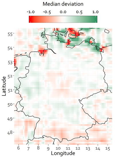
Figure 3.
Medians of grid-specific wind speed deviations (m/s) (forecast errors). Source: Own figure.
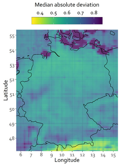
Figure 4.
Medians of grid-specific absolute wind speed deviations (m/s) (forecast errors). Source: Own figure.
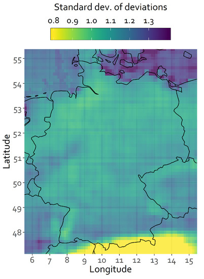
Figure 5.
Stand. deviations of grid-specific wind speed deviations (m/s) (forecast errors). Source: Own figure.

Figure 6.
The 99th percentiles of grid-specific absolute wind speed deviations (m/s) (forecast errors). Source: Own figure.
The median deviations are displayed in Figure 3. If a median substantially deviates from zero, wind speed estimations for this location are subjected to systematic errors, which could hint at differences in the models used to obtain forecast and actual values. Positive, green values represent a systematic overestimation of wind speeds and, conversely, negative, red values represent a systematic underestimation of wind speed. To make the differences more visible, the color scale was limited to the range of −1 to 1, containing 97.9% of values. All out-of-bound values were “squished” and represented by the end-of-range colors. This was done for the respective ranges shown in Figure 3, Figure 4, Figure 5 and Figure 6. Systematic forecast errors only occurred for few grid elements, which are mostly located near-shore and offshore. However, locations with installed offshore capacities (cf. Figure 2) do not seem to be affected by these systematic errors. Of the 1947 locations with installed capacities, 40.1% have median deviations between −0.05 and 0.05, 67.1% between −0.1 and 0.1 and 90.1% between −0.2 and 0.2.
The medians of absolute deviations, as a measure of average error magnitude, are displayed in Figure 4. The scale is limited to the range of 0.35–0.85, encompassing 96.2% of the medians. It can be observed that offshore locations are characterized by higher median absolute deviations, especially the Baltic Sea. Offshore locations with installed capacities, however, are characterized by smaller medians than offshore locations without capacities and near-shore locations, some of which show large median absolute deviations. In contract, most onshore locations have smaller medians, most noticeably the north of Germany, the area with the greatest share of installed onshore wind capacity.
The standard deviations of all location-specific deviations are displayed in Figure 5. They represent the variance of deviations. Overall, 93.4% of the standard deviations fall into the range between 0.8 and 1.4, the limits of the color scale. The magnitudes of standard deviations assume a similar geographic distribution compared to the median absolute deviations. They are larger offshore and comparatively smaller onshore, with the exception of some near-shore locations.
Lastly, Figure 6 shows the 99th percentiles of absolute deviations. This serves to evaluate the magnitude of unlikely deviations, while ignoring outliers, which are assumed to be contained in the highest one percent. Overall, 96% of the values fall into the range between 2 and 4.75, limiting of the color scale. Offshore and near-shore locations have higher extreme values than onshore locations. This difference is not as distinct for the North Sea.
4.1.1. Difference in Wind Speed Uncertainties for Offshore and Onshore Locations
The combination of higher median absolute deviations and standard deviations suggests that offshore locations are subjected to larger average forecast errors and higher variation of forecast errors. This, in turn, can translate into greater day-ahead uncertainties and forecast errors regarding the available wind energy. This effect could be amplified by two offshore wind characteristics, which can be observed in Figure 7.

Figure 7.
Average of local, actual wind speeds of the available dataset at a height of 90 m in relation to the standard deviation of wind speed deviations. The point size corresponds to the installed capacity for each onshore and (black-rimmed) offshore location and the color corresponds to the median absolute deviation. Source: Own diagram.
First, offshore wind capacities are geographically more concentrated, which means greater installed capacities for the predefined grid locations. This is due to large wind turbines and high accumulation of turbines into wind parks at few offshore locations. This translates into a higher capacity affected by forecast errors simultaneously. Second, wind speeds are, on average, higher for offshore than onshore locations. Due to the cubic relation between wind speed and energy output, a marginal deviation translates into larger output changes at higher wind speeds. Figure 7 also shows that locations with greater average wind speeds are subjected to greater standard deviations and higher median absolute forecast deviations. These characteristics affect all offshore wind locations, reiterating the previously described insights. Locations with very large median absolute deviations are all near-shore locations. The color scale is limited to 1, but some near-shore locations exceed this limit. These locations are also characterized by high variance in deviations, seven of which are not displayed in Figure 7 because their standard deviations are greater than the upper limit. The capacities of near-shore locations with median absolute deviations exceeding 0.8 amount to over 1.1 GW. Most of these locations also have standard deviations greater than 1.2. This means that there is a substantial part of onshore capacities that is subjected to large wind speed uncertainties.
While large offshore wind capacities can be affected by high wind speed deviations simultaneously, this can also be the case for onshore locations. The reason for this is not the high consolidation of wind turbines in few locations, but the fact that large onshore areas can be affected by similar wind speed deviations at the same time. Figure 8 and Figure 9 show the actual wind speeds and the wind speed forecast errors for 8 September 2018 at 12:00. There are two distinct characteristics of this situation. First, there are medium to high wind speed for all locations except south Germany. Second, almost all of Germany is subjected to wind speed overestimations, some of which are very large. This means that the vast majority of onshore wind turbines could generate less electricity than anticipated by the day-ahead forecast. Consequently, the overall available wind energy could be substantially affected due to the magnitude of wind speed forecast errors and the high sensitivity of wind power output to wind speed deviations at medium and high wind speeds. This extreme example illustrates that onshore wind power, despite the scattered nature of its capacities, also has the potential to introduce large uncertainties into the aggregated wind energy forecasts.
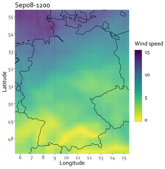
Figure 8.
Actual wind speeds on 8 September 2018 at 12:00. Source: Own figure.

Figure 9.
Wind speed forecast errors on 8 September 2018 at 12:00. Source: Own figure.
Lastly, the spatial correlation of wind speed deviations can provide insights into the simultaneity of forecast errors in relation to the geographical distance. Figure 10 shows the correlations between all locations with installed capacities and the corresponding distance between the locations. All pairs with an offshore location are displayed in black.

Figure 10.
Spatial correlation of wind speed deviations between locations with installed capacities in relation to their distance. Source: Own diagram.
Three distinct features can be derived from the spatial correlation analysis. First, the correlation decreases at a declining rate in relation to the distance. While there are more frequent outliers below a distance of 200 km, the bandwidth of correlations narrows for larger distances. Second, for distances exceeding 150 km, offshore locations show smaller correlation values, on average. This suggests that offshore wind speed deviations are more independent from errors at other locations. Conversely, the forecast errors of onshore locations correlate with other locations to a larger degree, suggesting that simultaneous over- and underestimations are a more pronounced phenomenon on land. In combination with the above-described effect on the available wind energy, large over- or underestimations of aggregated wind energy could be a larger issue for onshore wind energy. The third aspect is the virtual absence of negative correlations. This hints at the fact that over- and underestimations could be a relatively frequent phenomenon.
4.1.2. The Effect of Interpolation on the Results
As mentioned in Section 3, interpolation can introduce estimation errors because large short-term wind speed fluctuations between the 3-h forecast intervals are not accounted for. To evaluate if interpolation substantially alters the location-specific distributions of deviations, the median deviations, median absolute deviations, standard deviations and 99th percentiles of deviations are re-estimated, only considering non-interpolated time stamps, i.e., 0:00, 3:00, 6:00, etc.
The resulting distributions are displayed in Figure 11. It can be observed that interpolation leads to slightly more positive median deviations. The median absolute deviations also slightly increase through interpolation for some locations. However, the shift takes place at the center of the distribution, within the range of 0.25–0.7. Bins at the distribution tails are largely unaffected. In addition, interpolation leads to a slight decrease in standard deviations. Again, the shift occurs predominantly at the center of the distributions, within the range of 1.0–1.3. Lastly, interpolated deviations appear to be less extreme, as the 99th percentiles of non-interpolated deviations are higher for some locations.
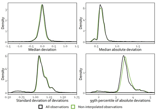
Figure 11.
Empirical density plots of median deviations, median absolute deviations, standard deviations of deviations and 99th percentiles of deviations, for all values and only for non-interpolated observations. Source: Own diagram.
For all four statistical characteristics of grid-specific deviations, there is a large overlap of the distributions of non-interpolated values and all values. While deviations seem to be slightly increased through interpolation, the distributions are characterized by slightly smaller standard deviations and lower extreme values. Consequently, systematic changes stemming from interpolation are expected to be insubstantial for this analysis.
4.2. Distribution Characteristics of Wind Speed Forecast Errors for Onshore and Offshore Locations
To investigate the distributions of onshore and offshore wind speed deviations, the installed capacities for each location have to be considered. Effectively, this only selects locations with installed capacities (1947 locations in total) and accounts for the relative importance of the particular location. The size of wind energy capacities will determine how much uncertainty local forecast errors will introduce into the energy system.
For this, a capacity-weighted sample was drawn from each location-specific distribution of deviations. To sufficiently represent local deviations, the capacity of the location (in MW) was multiplied by 30 and the resulting amount of observations was randomly selected from the respective distribution. For instance, for a location with 20 MW, 600 observations were drawn from the 18,192 observations of the respective location. A minimum of 30 observations was selected, even when capacities were below 1 MW. Weighting the capacities by 30: (1) ensured that for locations with large capacities not all available observations were drawn; and (2) kept the total amount of drawn observations manageable, as there are over 35 million observations in total.
To ensure that the subsamples were representatives of the overall location-dependent empirical distributions, the two-sample Kolmogorov–Smirnov Test was conducted for each random sampling. If the null hypothesis of the test, i.e., equal distribution of the subsample and overall location-specific empirical distribution, was rejected at the 5% significance level, the random sample was redrawn. Additionally, the Cucconi Test was conducted, which tests for the equality of location and scale. It is considered to be a more powerful non-parametric test [60,61]. Lastly, all subsamples were combined, separately for onshore and offshore locations. The distribution of the resulting sample is a representation of how often 1 MW of installed wind energy capacity is subjected to a certain deviation. It is important to note that no geographical correlations of wind speeds were taken into account. Therefore, the distribution does not represent the simultaneity of forecast error events.
Table 1 displays the moments of the two resulting distribution. While both distributions are characterized by an accumulation of values close to the mean and heavy tails (kurtosis > 6), the standard deviation of the offshore distribution is larger. Offshore wind capacities are subjected to absolute wind speed deviations greater than 1 m/s about 32.6% of the time, compared to 28.8% for wind onshore. In addition, absolute deviations exceed 3 m/s, 5 m/s and 10 m/s at offshore locations more often than at onshore locations. The 0.5th-percentile and 99.5th-percentile are closer to the mean for onshore compared to offshore. This suggests that the offshore distribution for wind speed forecast errors is tail-heavier.

Table 1.
Onshore and offshore distribution characteristics of wind speed deviations (m/s).
5. Model-Based Analysis of Aggregated Wind Energy Forecasts
The previous part describes characteristics of offshore locations: larger and more variable wind speed forecast errors in combination with higher average wind speeds and more consolidated capacities. The third part of this analysis served to evaluate if these characteristics introduce more uncertainty into the energy system, in form of greater and more frequent deviations from the energy output forecast.
To evaluate the effect of greater offshore capacities, the location-specific wind speed time series were translated into power output. Equation (4) describes how the wind speeds at a height of 10 m, , were scaled up for each grid element i. This required the location-specific roughness as described in Section 3. Furthermore, the capacity-weighted height of each grid element was used to determine to what height the wind speeds was scaled up. Wind turbines for which no hub height was available were assigned the average hub height of their commission year. If no date regarding the initiation of operation was available, the average hub height was assigned.
The resulting height-scaled wind speed time series were subsequently translated into aggregated power outputs. This was done using an Extremely Randomized Trees (or Extra Trees) Regressor Model. Extra Trees is a further randomized form of Random Forests, which is an ensemble of Decision Trees. Random Forests: (1) only consider a random subset of features when looking for the best feature to split a node; and (2) create an array of Decision Trees, taking advantage of the fact that a group of predictors often outperforms an individual predictor. Extra Trees further randomizes this procedure by randomly choosing the threshold for splitting, or rather picking the best split among random splits, as opposed to finding the optimum threshold, which is done by Random Forests [62,63].
The model was trained, using a subset of actual and forecast scaled-up wind speeds for January to September 2018, created through stratified sampling to ensure that the training set (90% of observations) and test set (10% of observation) match the overall dataset in terms of the target value’s distribution. For stratified sampling, the target values, i.e., aggregated energy, were divided by 1000 and rounded up to the next integer value (ceiling function). In the consequent splitting of the dataset into training and test set, an equal or nearly equal distribution of the target value “categories” was ensured. The target values are the actual and forecast, day-ahead wind energy amounts from the ENTSO-E Transparency Platform, which are seen as the closest approximation of the real values [64]. The timeframe was chosen because, regarding the wind speed data, it was the latest available at time of retrieval. Second, it is closest to the installed capacities at the end of 2018. In total, 13,006 observations are available (2 × 6551 hourly values with 96 NAs).
For the estimation of aggregated wind energy, not only the local wind speeds were taken into account but also their squared value . In addition, the location-specific capacities served as an explanatory variable, and was, in addition, multiplied by the wind speed variables. The combination, displayed in Equation (5), resembles a binomial, parametric model of the power curve between (cut-in wind speed) and (rated wind speed) [65] and was created for all 1947 locations with installed capacities (cf. Section 4.2).
The -parameters can be estimated if information exists on and for each location, or rather each turbine [65]. Since this information, however, was not available, the Extra Trees Regressor Model was deployed to estimate all -parameters. The estimations were based on regression analyses, thus the parameters were computed jointly, parsing the effect of one explanatory variable by holding all other effects constant, Note that if estimating the coefficients across all observations, would have to be zero to correctly constitute that power output is zero in the absence of wind. The estimation of -parameters, however, depends on the leaf node of the (randomized) decision tree(s). Due to the possibility of having only nonzero wind speed observations in a particular leaf node, was added for each location to provide extra flexibility for the model. In a normal decision tree, this would lead to excessive overfitting, which is part of the reason the proposed model is regularized.
Note that the only variables used for the estimation were wind speeds and capacities. Hub heights were the single technical turbine information, incorporated through the scaling of wind speeds. This approach was decoupled from any other turbine-specific factors, such as altitude, turbine type and interactions with other turbines (cf. [39]), which would be necessary for bottom-up approaches. Interaction within wind parks, e.g., wake effects, could not be modeled due to the aggregation of wind turbines and parks and the data availability (see Section 3).
The Extra Trees Regressor Model can be regularized to ensure adequate out-of-sample performance [62,63]. This is important for two reasons. First, because the training data had to be close to the date of installed capacities, the chosen model was applied to out-of-sample wind speed observations, i.e., July to November 2016 and February to December 2017. Second, the goal of this analysis was to measure the effect of changing wind capacities on the overall energy output, both for forecasts and actual values. Because capacities serves as an explanatory variable, changing them can be seen as applying the model coefficients out of sample. Using a standard model, such as Ordinary Least Squares Regression, could lead to overfitted, skewed parameters that perform poorly on a new or altered dataset.
5.1. Specifications and Performance of the Model
A key challenge for regularized models is finding the right hyperparameters. Extra Trees has an array of hyperparameters, which can be used to “tune” the model. Table 2 displays the tested combinations of hyperparameters and the corresponding root mean squared error (RMSE) for the training set and test set. The RMSE is the target value of the minimization model. For the training set, the average RMSE of the three cross-validations is shown.
Table 2.
Root mean squared errors (RMSEs) for test and training set (in parentheses) and duration of model training (in seconds) for different hyperparameters.
The greatest gains in model accuracy can be observed from increasing the maximum leaf nodes. This effect is greater for the training set than for the test set. A possible reason for the difference between RMSEs of the test and training set is the limited amount of observations that is small compared to the amount of estimators. The ensuing gap between training RMSE and test RMSE can hint at overfitting, which was not confirmed by further increasing the maximum leaf nodes. Within the tested range of maximum leaf nodes, the test set RMSE remained nearly constant from 5000 to 10,000 nodes. For some combinations of hyperparameters the test set RMSE slightly increased at a maximum of 10,000, which is why this maximum was not further increased. Hence, the more likely reason for the gap between test set RMSE and training set RMSE is a relatively small amount of observations. Increasing the minimum sample size for each leaf node did close the gap but led to worse performance for both. Thus, no minimum was set.
The number of estimators has a limited positive effect on model accuracy. Increasing the limit on the maximum amount of features from 1000 to 2500 had mixed but small effects on the test set RMSEs, which is why not more than a maximum of 2500 features was considered for the splitting of nodes. Increasing the amount of folds for cross-validation did not improve out-of-sample performance, which is why a three-fold cross-validation was applied universally. For these reasons, the Extra Trees Model with 2500 as a maximum amount of features, 250 estimators and a maximum of 10,000 leaf nodes was selected, which corresponds with a test set RMSE of 1597 and a test set mean squared error (MAE) of 1145.
To illustrate the performance of the selected Extra Trees model, the wind speed observations for September 2018 were transformed into aggregated wind power output. In Figure 12 and Figure 13, one can observe that the model transformed the wind speed data into actual wind energy values and day-ahead forecasts in a manner that closely matches the aggregated ENTSO-E values for most timesteps with only few exceptions. It is important to mention that the errors for September (Actual: RMSE = 803 and MAE = 511, Day-ahead: RMSE = 749 and MAE = 496) lie below the errors for the stratified test set, because it includes observations from the training and test set.

Figure 12.
September ERA5 wind speed time series transformed into aggregated wind energy output compared with actual ENTSO-E wind energy values. Source: Own diagram.

Figure 13.
September CAMS wind speed time series transformed into aggregated wind energy output compared with day-ahead ENTSO-E wind energy values. Source: Own diagram.
To compare the model performance, the estimated time series and ENTSO-E time series of wind energy are transformed into capacity factors (CFs), according to the overall installed capacity at the end of 2018. In addition, the onshore CF time series of EMHIRES [66,67] and Renewables Ninja [68,69] were retrieved and compared to the ENTSO-E values. Subsequently, the hourly differences between the ENTSO-E CFs and the CFs of the (1) estimated time series; (2) EMHIRES time series; and (3) Renewables Ninja time series, respectively, were computed.
Table 3 displays the resulting MAEs for all three time series, from 2012 up to the year available at the time of download. For onshore energy, the MAEs of capacity factor for Renewables Ninja range from 2.4% to 2.9% and for EMHIRES from 4.1% to 5.3%. The overall MAE for of the trained model results is 0.8%. As mentioned above, there is a gap between the test set and training set performance (measured by the RMSE). Naturally, this is also the case for the MAE when evaluating the capacity factors. Here, the training set MAE is 0.7% and the test set MAE is 1.8%. Under the assumption that the model is supposed to perform well on out-of-sample data, the test set MAE is the more appropriate value to compare model performance with.
Table 3.
Comparison of mean absolute errors (MAEs) for capacity factors.
The results suggest the Extra Trees model slightly outperformws the capacity factors retrieved from Renewables Ninja. The difference is greater compared to EMHIRES CFs. Note that the trained Extra Trees model contains onshore and offshore wind, while for EMHIRES and Renewables Ninja the capacity factors are listed separately. With MAEs around 10% for offshore CFs, combining onshore and offshore CFs would worsen the overall MAEs of EMHIRES and Renewables Ninja. It is important to keep in mind that the proposed model was only trained and evaluated on a relatively short amount of time. However, as input parameters, local wind speeds, capacities and hub heights suffice to generate wind energy amounts with small deviations from real amounts, when tested on out-of-sample data.
5.2. Model Results for Onshore and Offshore Capacity Expansion
The corresponding coefficients of the chosen Extra Tree Model were used to estimate the aggregated wind energy for all observations, i.e., all available 25 months of wind speed data. This was done for forecast and actual values, separately. Then, the deviations between the two time series were analyzed. This analysis was performed for three cases:
- Base case: Actual installed capacities were used.
- Offshore expansion: All offshore capacities were multiplied by the same factor to result in an additional 5 GW of offshore capacity.
- Onshore expansion: All onshore capacities were multiplied by the same factor to result in an additional 5 GW of onshore capacity.
While the base case served as a comparison, the analysis focused on the offshore expansion. It was important to also evaluate onshore expansion, the second counter-factual case. Greater deviations in total wind energy forecasts could simply stem from the expansion of wind generation capacity in general. Cases 2 and 3 allowed for parsing the effect of offshore and onshore capacity expansion. For comparison, the ENTSO-E deviations for January to September 2018, the target values for the Extra Trees model, were juxtaposed throughout the evaluation. This served to validate the model performance regarding the distribution of obtained wind energy forecast errors.
The model-based results for all three cases are displayed in Figure 14. The moments of the distributions are summarized in Table 4. Overall, the distribution of deviations in the base case is similar to the ENTSO-E deviations. The model results are characterized by a slight positive skewness and a higher kurtosis, expressed by more frequent high deviations. Note that the base case values encompass a longer time frame, i.e., 25 months with available wind speed data, which can also lead to deviations from the ENTSO-E distribution.

Figure 14.
Categorical shares of absolute wind energy forecast errors for: (1) ENTSO-E deviations (January–September 2018); and forecast errors resulting from the Extra Trees Model for: (2) the base case; (3) an additional 5 GW of offshore wind capacity; and (4) an additional 5 GW of onshore wind capacity, respectively. Source: Own diagram.
Table 4.
Distribution characteristics of wind energy forecast errors (GW).
Noticeably, the expansion of wind energy capacity leads to fewer absolute deviations below 0.5 GW and between 0.5 and 1 GW, and more absolute deviations for all categories above 1 GW and below 5 GW. The second effect is more pronounced for offshore than for onshore expansion in most categories of deviation magnitude (the exception is the range from 3.5 GW to 4 GW, in which offshore expansion has slightly fewer occurrences than the base case).
Interestingly, onshore expansion shows a higher share in the category ≥5 GW, compared to offshore expansion, which barely deviates from the base case in this category. Section 4.1 describes: (1) the high variability of near-shore wind speeds; and (2) the simultaneous over- or underestimation of wind speeds of many onshore locations. Due to the greater spatial correlation of wind speed forecast errors at onshore locations (Section 4.1), the second characteristic is likely to be the leading cause for more frequent extreme errors in wind energy forecasts in the case of onshore capacity expansion. This higher tail-heaviness is confirmed by a higher kurtosis (Table 4) for the onshore capacity expansion case, which deviates even further from a normal distribution than the base case. The offshore capacity expansion case shows a lower kurtosis than the base case. This is due to fewer small deviations, more frequent medium or high deviations but a very small decrease in very high deviations (comparable kurtosis values for wind energy forecast errors were found by Bludszuweit et al. [70]).
In all cases, the distributions are right-skewed, resulting in a positive mean. This suggests that extreme overestimations of wind energy are more frequent than extreme underestimations. These events, however, are rare and the differences between onshore and offshore expansion are small for very high deviations (≥5 GW) and minute for extreme deviations (≥10 GW).
Note that this analysis is based on wind speed forecasts. As these forecasts are mainly relevant for weather forecasting, it can be assumed that forecasts are derived under the objective of being unbiased. However, planners responsible for wind energy feed-in may have an incentive for underestimating their feed-in [34] due to the shape of the merit-order curve and the resulting impact on power prices. An (ex-post) underestimation in general results in higher balancing costs and thus an ex-ante underestimation, resulting in a lower risk of having a real underestimation, is favorable for the planner. This possibility is not considered in this analysis though.
6. Conclusions
The results indicate that offshore locations are subjected to more uncertain wind speed forecasts in the form of higher deviations, more variance in deviations and slightly higher extreme deviations. Additionally, offshore wind capacities are more consolidated and are subjected to higher average wind speeds, amplifying the effect of higher and more variable wind speed errors on wind energy forecast errors. Consequently, the expansion of offshore wind capacity increases the frequency of medium to high wind energy forecast errors, namely deviations in the range of 1–5 GW, more substantially than the expansion of onshore wind capacity. The results suggest that extreme forecast errors, however, are more frequent when onshore wind capacity is expanded. This phenomenon likely stems from similar wind speed forecast errors that simultaneously affect many onshore locations and possibly from near-shore locations, characterized by the highest wind speed uncertainties in terms of magnitude and variability. These different impacts from onshore and offshore wind energy on the energy system and, in turn, on energy prices, including self-marginalization, have to be considered when targeting higher shares of renewable energies.
The developed model can serve as a tool for quantifying the magnitude and probability of wind energy forecast errors under different wind capacity expansion paths. Taking into consideration the planned German offshore wind parks, which will add substantial capacities in the coming years, day-ahead markets will likely be subjected to greater uncertainties regarding available wind energy. On a market level, this could imply less assurance in the unit commitment and economic feasibility of conventional power plants, as well as greater challenges for the operators of wind parks. On an operative level, the greater magnitude and variability of forecast errors of offshore wind speeds can lead to a heightened demand for preventative and curative measures, such as redispatch and curtailment, amplified by the more centralized feed-in of offshore wind energy at few nodes in the grid. The possible economic repercussions for market participants and power system operators have to be accounted for when planning the integration of weather-dependent renewable energies, which especially pertain to wind energy as a nearly omnipresent and volatile source of renewable power supply.
The performance of the proposed Extra Trees model suggests that it is a viable, promising method to compute aggregated amounts of wind energy, only relying on local wind speeds, in combination with location-specific capacities and hub height data, as input. The performance should be validated on longer time spans. Furthermore, bottom-up, fundamental modeling of wind power feed-in, using regional plant capacity and data including power curves of wind plants for converting wind-speeds into energy feed-in, would be an interesting comparison (and further performance benchmark) for the Extra Trees model. The advantage of the Extra Trees model lies in the decreased effort to gather data in comparison to bottom-up modeling. Based on the in-depth analysis, it would be worth evaluating the impact on electricity prices as well as balancing needs in a future energy system. Lastly, the discussed performance and generalizability of the model are promising features for extending its range of application. Rather than transforming wind speeds into wind energy, it is worth investigating if the proposed model can also serve as a forecasting tool, i.e., predicting actual wind energy amounts (for day D) based on day-ahead wind speeds or even based on two-day-ahead wind speeds. If performance is up to par, the model could enhance accurate short-term anticipation of available wind energy amounts with parsimonious data requirements.
Author Contributions
Data curation, methodology, software, formal analysis, visualization, investigation and project administration were done by D.S.; conceptualization, validation, writing of original draft and editing were done by D.S. and D.M.; and supervision and funding acquisition were by D.M.
Funding
The authors gratefully acknowledge the funding by the German Federal Ministry for Economic Affairs and Energy (BMWi) in the project “Long-term Capacity Planning and Short-term Optimization of the German Electricity System Within the European Context” (LKD-EU, 03ET4028C).
Acknowledgments
The authors would like to thank Benjamin Kirchner for the compilation of wind power plant data.
Conflicts of Interest
The authors declare no conflict of interest. The funders had no role in the design of the study; in the collection, analyses, or interpretation of data; in the writing of the manuscript, or in the decision to publish the results.
Abbreviations
The following abbreviations are used in this manuscript:
| abs. | absolute |
| CAMS | Copernicus Atmosphere Monitoring Service |
| CF | capacity factor |
| dev. | deviation |
| ECMWF | European Centre for Medium-Range Weather Forecasts |
| EMHIRES | European Meteorological derived high resolution renewable energy source generation time series |
| ENTSO-E | European Network of Transmission System Operators for Electricity |
| ERA5 | 5th generation of ECMWF Reanalysis |
| GW | gigawatt |
| MAE | mean absolute error |
| MW | megawatt |
| RMSE | root mean squared error |
References
- State Office for the Environment of Baden-Württemberg (LUBW). Data and Map Service of LUBW. 2018. Available online: http://udo.lubw.baden-wuerttemberg.de/public/pages/selector/index.xhtml (accessed on 20 December 2018).
- Bavarian Ministry of Economic Affairs, Regional Development and Energy. Energieatlas Bayern. 2018. Available online: https://geoportal.bayern.de/energieatlas-karten/ (accessed on 20 December 2018).
- Berlin Senate Department for Economics, Energy and Public Enterprises. Energieatlas Berlin. 2018. Available online: https://energieatlas.berlin.de/ (accessed on 20 December 2018).
- Ministry of Rural Development, Environment and Agriculture of the Federal State of Brandenburg. Geoportal Brandenburg. 2018. Available online: https://geoportal.brandenburg.de/startseite/ (accessed on 20 December 2018).
- Bremen Senator for Construction, Environment and Traffic. Wind Power Plants and Locations in Bremen. 2018. Available online: https://www.bauumwelt.bremen.de/umwelt/klima_und_energie/windenergie-24764 (accessed on 20 December 2018).
- Hamburg Ministry of Environment and Energy. Geo Services Hamburg. 2018. Available online: https://geodienste.hamburg.de/HH_WFS_Windkraftanlagen?VERSION=1.1.0&typename=app:wka (accessed on 20 December 2018).
- Hessian Agency for Nature Conservation, Environment and Geology. Wind Energy in Hesse. 2018. Available online: http://atlas.umwelt.hessen.de/servlet/Frame/atlas/energie/wind/windkraftanlagen.htm (accessed on 20 December 2018).
- Mecklenburg-Western Pomeranian Agency for the Environment, Nature Conservation and Geology. Map Services. 2018. Available online: https://www.lung.mv-regierung.de/insite/cms/umwelt/umweltinformation/gis/kartenportal/ (accessed on 20 December 2018).
- Ministry of Food, Agriculture and Consumer Protection Lower Saxony. Data Delivery Energieatlas Lower Saxony. 2018. Available online: https://www.energieatlas.niedersachsen.de/startseite/datenabgabe/ (accessed on 20 December 2018).
- North Rhine-Westphalia State Agency for Nature, Environment and Consumer Protection. Web Map and Feature Service. 2018. Available online: http://www.energieatlas.nrw.de/site/wms-und-wfs-dienste (accessed on 20 December 2018).
- Rhineland-Palatinate Energy Agency. Energieatlas Rhineland-Palatinate. 2018. Available online: https://www.energieatlas.rlp.de/earp/startseite/ (accessed on 20 December 2018).
- Saarland State Offices for Surveying, Geographic Information and rural Development. GeoPortal Saarland. 2018. Available online: http://geoportal.saarland.de/portal/de/startseite/ver-und-entsorgungnachrichtenwesen/ (accessed on 20 December 2018).
- Saxon State Office for the Environment, Agriculture and Geology. Wind Power Plants. 2018. Available online: https://www.umwelt.sachsen.de/umwelt/luft/43047.htm (accessed on 20 December 2018).
- Ministry for Regional Development and Transport of the State of Saxony-Anhalt. Energieatlas Saxony-Anhalt, Energy Infrastructure. 2018. Available online: https://www.sachsen-anhalt-energie.de/de/lsa-anlagenuebersicht.html (accessed on 20 December 2018).
- Federal Network Agency and State Agency for Agriculture, Environment and Rural Areas Schleswig-Holstein (LLUR). Wind Power Plants in Operation. 2018. Available online: https://www.arcgis.com/home/item.html?id=2fa8ef6956f54d5bb1df5e11db4e9e5c#data (accessed on 20 December 2018).
- Thuringian Administration Office. Geoportal Thuringia. 2018. Available online: http://www.geoproxy.geoportal-th.de/download-service/opendata/WKA_json.zip (accessed on 20 December 2018).
- The Wind Power. Germany Wind Farms. 2018. Available online: https://www.thewindpower.net/windfarms_list_en.php (accessed on 14 December 2018).
- 4C Offshore. Offshore Wind Farms in Germany. 2018. Available online: https://www.4coffshore.com/windfarms/windfarms.aspx?windfarmId=DE13 (accessed on 27 June 2019).
- Piwko, R.; Osborn, D.; Gramlich, R.; Jordan, G.; Hawkins, D.; Porter, K. Wind energy delivery issues [transmission planning and competitive electricity market operation]. IEEE Power Energy Mag. 2005, 3, 47–56. [Google Scholar] [CrossRef]
- Wang, Q.; Guan, Y.; Wang, J. A Chance-Constrained Two-Stage Stochastic Program for Unit Commitment With Uncertain Wind Power Output. IEEE Trans. Power Syst. 2012, 27, 206–215. [Google Scholar] [CrossRef]
- Xiong, P.; Jirutitijaroen, P.; Singh, C. A Distributionally Robust Optimization Model for Unit Commitment Considering Uncertain Wind Power Generation. IEEE Trans. Power Syst. 2017, 32, 39–49. [Google Scholar] [CrossRef]
- Bouffard, F.; Galiana, F.D. Stochastic Security for Operations Planning With Significant Wind Power Generation. In Proceedings of the 2008 IEEE Power and Energy Society General Meeting-Conversion and Delivery of Electrical Energy in the 21st Century, Pittsburgh, PA, USA, 20–24 July 2008; pp. 1–11. [Google Scholar] [CrossRef]
- Ummels, B.C.; Gibescu, M.; Pelgrum, E.; Kling, W.L.; Brand, A.J. Impacts of Wind Power on Thermal Generation Unit Commitment and Dispatch. IEEE Trans. Energy Convers. 2007, 22, 44–51. [Google Scholar] [CrossRef]
- Wang, J.; Shahidehpour, M.; Li, Z. Security-Constrained Unit Commitment With Volatile Wind Power Generation. IEEE Trans. Power Syst. 2008, 23, 1319–1327. [Google Scholar] [CrossRef]
- Tuohy, A.; Meibom, P.; Denny, E.; O’Malley, M. Unit Commitment for Systems With Significant Wind Penetration. IEEE Trans. Power Syst. 2009, 24, 592–601. [Google Scholar] [CrossRef]
- Makarov, Y.V.; Etingov, P.V.; Ma, J.; Huang, Z.; Subbarao, K. Incorporating Uncertainty of Wind Power Generation Forecast Into Power System Operation, Dispatch, and Unit Commitment Procedures. IEEE Trans. Sustain. Energy 2011, 2, 433–442. [Google Scholar] [CrossRef]
- Jiang, R.; Wang, J.; Guan, Y. Robust Unit Commitment With Wind Power and Pumped Storage Hydro. IEEE Trans. Power Syst. 2012, 27, 800–810. [Google Scholar] [CrossRef]
- Pozo, D.; Contreras, J. A Chance-Constrained Unit Commitment With an n-K Security Criterion and Significant Wind Generation. IEEE Trans. Power Syst. 2013, 28, 2842–2851. [Google Scholar] [CrossRef]
- Papavasiliou, A.; Oren, S.S. Multiarea Stochastic Unit Commitment for High Wind Penetration in a Transmission Constrained Network. Oper. Res. 2013, 61, 578–592. [Google Scholar] [CrossRef]
- Qadrdan, M.; Wu, J.; Jenkins, N.; Ekanayake, J. Operating Strategies for a GB Integrated Gas and Electricity Network Considering the Uncertainty in Wind Power Forecasts. IEEE Trans. Sustain. Energy 2014, 5, 128–138. [Google Scholar] [CrossRef]
- Mc Garrigle, E.V.; Leahy, P.G. Quantifying the value of improved wind energy forecasts in a pool-based electricity market. Renew. Energy 2015, 80, 517–524. [Google Scholar] [CrossRef]
- Doherty, R.; O’Malley, M. A new approach to quantify reserve demand in systems with significant installed wind capacity. IEEE Trans. Power Syst. 2005, 20, 587–595. [Google Scholar] [CrossRef]
- Weber, C. Adequate intraday market design to enable the integration of wind energy into the European power systems. Energy Policy 2010, 38, 3155–3163. [Google Scholar] [CrossRef]
- Von Selasinsky, A. The Integration of Renewable Energy Sources in Continuous Intraday Markets for Electricity; Technische Universität Dresden, Faculty of Business and Economics, Chair of Energy Economics: Dresden, Germany, 2016; Available online: https://nbn-resolving.org/urn:nbn:de:bsz:14-qucosa-202130 (accessed on 16 May 2019).
- Pinson, P.; Chevallier, C.; Kariniotakis, G.N. Trading Wind Generation From Short-Term Probabilistic Forecasts of Wind Power. IEEE Trans. Power Syst. 2007, 22, 1148–1156. [Google Scholar] [CrossRef]
- Barthelmie, R.; Murray, F.; Pryor, S. The economic benefit of short-term forecasting for wind energy in the UK electricity market. Energy Policy 2008, 36, 1687–1696. [Google Scholar] [CrossRef]
- Bitar, E.Y.; Rajagopal, R.; Khargonekar, P.P.; Poolla, K.; Varaiya, P. Bringing Wind Energy to Market. IEEE Trans. Power Syst. 2012, 27, 1225–1235. [Google Scholar] [CrossRef]
- Haessig, P.; Multon, B.; Ahmed, H.B.; Lascaud, S.; Bondon, P. Energy storage sizing for wind power: Impact of the autocorrelation of day-ahead forecast errors. Wind Energy 2015, 18, 43–57. [Google Scholar] [CrossRef]
- Brusca, S.; Capizzi, G.; Lo Sciuto, G.; Susi, G. A new design methodology to predict wind farm energy production by means of a spiking neural network–based system. Int. J. Numer. Model. Electron. Netw. Devices Fields 2017, 32, e2267. [Google Scholar] [CrossRef]
- Jónsson, T.; Pinson, P.; Madsen, H. On the market impact of wind energy forecasts. Energy Econ. 2010, 32, 313–320. [Google Scholar] [CrossRef]
- Ketterer, J.C. The impact of wind power generation on the electricity price in Germany. Energy Econ. 2014, 44, 270–280. [Google Scholar] [CrossRef]
- Kavasseri, R.G.; Seetharaman, K. Day-ahead wind speed forecasting using f-ARIMA models. Renew. Energy 2009, 34, 1388–1393. [Google Scholar] [CrossRef]
- Sanchez, I. Short-term prediction of wind energy production. Int. J. Forecast. 2006, 22, 43–56. [Google Scholar] [CrossRef]
- Sánchez, I. Adaptive combination of forecasts with application to wind energy. Int. J. Forecast. 2008, 24, 679–693. [Google Scholar] [CrossRef]
- Cheng, L.; Zang, H.; Ding, T.; Sun, R.; Wang, M.; Wei, Z.; Sun, G. Ensemble Recurrent Neural Network Based Probabilistic Wind Speed Forecasting Approach. Energies 2018, 11, 1958. [Google Scholar] [CrossRef]
- Zhou, J.; Sun, N.; Jia, B.; Peng, T. A Novel Decomposition-Optimization Model for Short-Term Wind Speed Forecasting. Energies 2018, 11, 1752. [Google Scholar] [CrossRef]
- Wang, R.; Li, J.; Wang, J.; Gao, C. Research and Application of a Hybrid Wind Energy Forecasting System Based on Data Processing and an Optimized Extreme Learning Machine. Energies 2018, 11, 1712. [Google Scholar] [CrossRef]
- Okumus, I.; Dinler, A. Current status of wind energy forecasting and a hybrid method for hourly predictions. Energy Convers. Manag. 2016, 123, 362–371. [Google Scholar] [CrossRef]
- Esteban, M.D.; Diez, J.J.; López, J.S.; Negro, V. Why offshore wind energy? Renew. Energy 2011, 36, 444–450. [Google Scholar] [CrossRef]
- LEANWIND. Driving Cost Reductions in Offshore Wind: The LEANWIND Project Final Publication. 2017. Available online: http://www.leanwind.eu/results/ (accessed on 30 April 2019).
- WindEurope. Wind Energy in Europe in 2018: Trends and Statistics. 2018. Available online: https://windeurope.org/about-wind/statistics/european/wind-energy-in-europe-in-2018/ (accessed on 30 April 2019).
- Copernicus Atmosphere Monitoring Service. CAMS Near-Real-Time. 2018. Available online: https://apps.ecmwf.int/datasets/data/cams-nrealtime/ (accessed on 5 December 2018).
- Copernicus Climate Change Service (C3S). ERA5: Fifth Generation of ECMWF Atmospheric Reanalyses of the Global Climate. C3S Climate Data Store (CDS). 2018. Available online: https://apps.ecmwf.int/data-catalogues/era5/?class=ea (accessed on 5 December 2018).
- Wickham, H. ggplot2: Elegant Graphics for Data Analysis; Springer: New York, NY, USA, 2009; Available online: http://ggplot2.org (accessed on 7 May 2019).
- Wickham, H. The Split-Apply-Combine Strategy for Data Analysis. J. Stat. Softw. 2011, 40, 1–29. [Google Scholar] [CrossRef]
- Komsta, L.; Novomestky, F. Moments: Moments, Cumulants, Skewness, Kurtosis and Related Tests; R Package Version 0.14; 2015; Available online: https://CRAN.R-project.org/package=moments (accessed on 7 May 2019).
- Pierce, D. ncdf4: Interface to Unidata netCDF (Version 4 or Earlier) Format Data Files; R Package Version 1.16; 2017; Available online: https://CRAN.R-project.org/package=ncdf4 (accessed on 7 May 2019).
- Garnier, S. viridis: Default Color Maps from ’matplotlib’; R Package Version 0.5.1; 2018; Available online: https://CRAN.R-project.org/package=viridis (accessed on 7 May 2019).
- Pedregosa, F.; Varoquaux, G.; Gramfort, A.; Michel, V.; Thirion, B.; Grisel, O.; Blondel, M.; Prettenhofer, P.; Weiss, R.; Dubourg, V.; et al. Scikit-learn: Machine Learning in Python. J. Mach. Learn. Res. 2011, 12, 2825–2830. [Google Scholar]
- Marozzi, M. Some notes on the location-scale Cucconi test. J. Nonparametric Stat. 2009, 21, 629–647. [Google Scholar] [CrossRef]
- Marozzi, M. Nonparametric Simultaneous Tests for Location and Scale Testing: A Comparison of Several Methods. Commun. Stat.-Simul. Comput. 2013, 42, 1298–1317. [Google Scholar] [CrossRef]
- Géron, A. Hands-On Machine Learning with Scikit-Learn and TensorFlow: Concepts, Tools, and Techniques to Build Intelligent Systems; O’Reilly Media, Inc.: Sebastopol, CA, USA, 2017. [Google Scholar]
- Geurts, P.; Ernst, D.; Wehenkel, L. Extremely randomized trees. Mach. Learn. 2006, 63, 3–42. [Google Scholar] [CrossRef]
- ENTSO-E. Transparency Platform: Actual Generation per Production Type, Generation Forecasts for Wind and Solar and Installed Capacity per Production Type. 2018. Available online: https://transparency.entsoe.eu/ (accessed on 12 January 2019).
- Sohoni, V.; Gupta, S.; Nema, R. A critical review on wind turbine power curve modelling techniques and their applications in wind based energy systems. J. Energy 2016, 2016. [Google Scholar] [CrossRef]
- European Commission. EMHIRES Datasets: 30 Years of Wind Power Capacity Factors at Country Level, Onshore. 2018. Available online: https://setis.ec.europa.eu/EMHIRES-datasets (accessed on 15 October 2018).
- Gonzalez Aparicio, I.; Zucker, A.; Careri, F.; Monforti, F.; Huld, T.; Badger, J. EMHIRES dataset; Part 1: Wind power generation. Eur. Union JRC Sci. Hub 2016, 24. [Google Scholar] [CrossRef]
- Renewables.ninja. Hourly Wind Capacity Factors. 2018. Available online: https://www.renewables.ninja/downloads (accessed on 15 October 2018).
- Staffell, I.; Pfenninger, S. Using bias-corrected reanalysis to simulate current and future wind power output. Energy 2016, 114, 1224–1239. [Google Scholar] [CrossRef]
- Bludszuweit, H.; Domínguez-Navarro, J.A.; Llombart, A. Statistical Analysis of Wind Power Forecast Error. IEEE Trans. Power Syst. 2008, 23, 983–991. [Google Scholar] [CrossRef]


© 2019 by the authors. Licensee MDPI, Basel, Switzerland. This article is an open access article distributed under the terms and conditions of the Creative Commons Attribution (CC BY) license (http://creativecommons.org/licenses/by/4.0/).