Short-Term Electricity Demand Forecasting Using Components Estimation Technique

Abstract

Currently, in most countries, the electricity sector is liberalized, and electricity is traded in deregulated electricity markets. In these markets, electricity demand is determined the day before the physical delivery through (semi-)hourly concurrent auctions. Hence, accurate forecasts are essential for efficient and effective management of power systems. The electricity demand and prices, however, exhibit specific features, including non-constant mean and variance, calendar effects, multiple periodicities, high volatility, jumps, and so on, which complicate the forecasting problem. In this work, we compare different modeling techniques able to capture the specific dynamics of the demand time series. To this end, the electricity demand time series is divided into two major components: deterministic and stochastic. Both components are estimated using different regression and time series methods with parametric and nonparametric estimation techniques. Specifically, we use linear regression-based models (local polynomial regression models based on different types of kernel functions; tri-cubic, Gaussian, and Epanechnikov), spline function-based models (smoothing splines, regression splines), and traditional time series models (autoregressive moving average, nonparametric autoregressive, and vector autoregressive). Within the deterministic part, special attention is paid to the estimation of the yearly cycle as it was previously ignored by many authors. This work considers electricity demand data from the Nordic electricity market for the period covering 1 January 2013–31 December 2016. To assess the one-day-ahead out-of-sample forecasting accuracy, Mean Absolute Percentage Error (MAPE), Mean Absolute Error (MAE), and Root Mean Squared Error (RMSE) are calculated. The results suggest that the proposed component-wise estimation method is extremely effective at forecasting electricity demand. Further, vector autoregressive modeling combined with spline function-based regression gives superior performance compared with the rest.

1. Introduction

Liberalization of the energy sector, changes in climate policies, and the upgrade of renewable energy resources have completely changed the structure of the previous strictly-controlled energy sector. Today, most energy markets have been liberalized and privatized with the purpose of gaining consistent and inexpensive facilities for power trades. Within the energy sector, the liberalization of the electricity market has also introduced new challenges. In particular, electricity demand and price forecasting have become extremely important issues for producers, energy suppliers, system operators, and other market participants. In many electricity markets, electricity demand is fixed a day before the physical delivery by concurrent (semi-)hourly auctions. Further, electricity cannot be stored in an efficient manner, and the end-user demand must be satisfied instantaneously; thus, accurate forecast for electricity demand is crucial for effective power system management [1,2].

The electricity demand forecast can be broadly divided into three time horizons: (a) short-term, (b) medium-term, and (c) long-term load forecasting. Long-Term Load Forecast (LTLF) includes horizons from a few months to several years ahead. LTLF is generally used for planning and investment profitability analysis, determining upcoming sites, or acquiring fuel sources for production plants [3]. Medium-Term Load Forecast (MTLF) normally considers horizons from a few days to months ahead and is usually preferred for risk management, balance sheet calculations, and derivatives pricing [4]. Finally, Short-Term Load Forecast (STLF) generally includes horizons from a few minutes up to a few days ahead. In practice, the most attention in electricity load forecasting has been paid to STLF since it is an essential tool for the daily market operations [5].

However, electricity demand forecasting is a difficult task due to the features demand time series exhibit. These features include non-constant mean and variance, calendar effects, multiple periodicities, high volatility, jumps, etc. For example, the yearly, weekly, and daily periodicities can be seen from Figure 1. The weekly phase is comprised of comparatively lower variation in the data. The load curves are comparatively different on different days of the week, and the demand varies throughout the day. The demand is high on weekdays as compared to weekends. Moreover, electricity demand is also affected by calendar effects (bank/bridging holidays) and by seasons. In general, the demand is considerably lower during bank holidays and bridging holidays (a day among two non-working days). From the figure, high volatility in electricity demand can also be observed in almost all load periods. In addition, different environmental, geographical, and meteorological factors have a direct effect on electricity demand. Further, as electricity is a secondary source of energy, which is retrieved by converting prime energy sources like fossil fuels, natural gas, solar, wind power, etc. [6], the cost related to each source is different. Thus, a consistent electricity supply mechanism for different levels of demand with short periods of high and rather longer periods of moderate demand is necessary.

To account for the different features of the demand series, in the last two decades, researchers suggested different methods and models to forecast electricity demand [7,8,9,10,11]. For example, the work in [12] proposed a semi-parametric component-based model consisting of a non-parametric (smoothing spline) and a parametric (autoregressive moving average model) component. Exponential smoothing techniques are also widely used in forecasting electricity demand [13,14]. Multiple equations time series models, e.g., the Double Seasonal Autoregressive Moving Average (DSARIMA) model, the Double Holt–Winters (D-HW) model, and Multiple Equations Time Series (MET) approaches are also used for short-term load forecasting [15,16]. Regression methods are easy to implement and have been widely used for electricity demand forecasting in the past. For example, the work in [17] used parametric regression models to forecast electricity demand for the Turkish electricity market. Some authors included exogenous variables in the time series models to improve the forecasting performance [18,19,20]. Several researchers compared the classical time series models and computational intelligence models [21,22,23]. For example, the work in [24] compared the Seasonal Autoregressive Moving Average (SARIMA) and Adaptive Network-based Fuzzy Inference System (ANFIS) models. For short-term load forecasting, the work in [25] introduced a new hybrid model that combines SARIMA and the Back Propagation Neural Network (BPNN) model. Some authors suggested the use of functional data analysis to predict electricity demand [26,27,28]. The main idea behind this approach is to consider the daily demand profile as a single functional object; thus, functional approaches can be applied to electricity load series. Other approaches used for demand forecasting can be seen in [29,30,31,32,33]. Apart from the forecasting models, Distributed Energy Resources (DERs) that are directly connected to a local distribution system and can be used for electricity producing or as controllable loads are also discussed in the literature [34,35]. DERs include solar panels, combined heat and power plants, electricity storage, small natural gas-fueled generators, and electric water heaters.

The main objective of this work is to compare different modeling techniques for electricity demand forecasting. The main attention is paid to the yearly cycle, which in many cases is ignored. The authors suggest to estimate jointly the effect of the long-term trend and yearly cycle using one component [36,37]. In practice, however, the yearly component shows regular cycles, while the long-term component highlights the trend structure of the data. Thus, these two components must be modeled separately [26]. Further, in our case, some pilot analyses suggested that modeling these two components separately can significantly improve the forecasting results. Thus, the main contribution of this paper is the thorough investigation of the impact of yearly component estimation on one-day-ahead out-of-sample electricity demand forecasting. Within the framework of the components estimation method, we compare models in terms of forecasting ability considering both univariate and multivariate, as well as parametric and non-parametric models. Moreover, for the considered models, the significance analysis of the difference in predication accuracy is also conducted.

The rest of the article is organized as follows: Section 2 contains a description of the proposed modeling framework and of the considered models. Section 3 provides an application of the proposed modeling framework. Section 4 contains a summary and conclusions.

2. Component-Wise Estimation: General Modeling Framework

The main objective of this study is to forecast one-day-ahead electricity demand using different forecasting models and methods. To this end, let log$\left(D_{t,j}\right)$ be the series of the log demand for the $t^{\mathrm{th}}$ day and the $j^{\mathrm{th}}$ hour. Following [28,33], the dynamics of the log demand, log$\left(D_{t,j}\right)$, can be modeled as:

$$\log \left(D_{t,j}\right)=F_{t,j}+R_{t,j}$$

(1)

That is, the log$\left(D_{t,j}\right)$ is divided into two major components: a deterministic component $F_{t,j}$ and a stochastic component $R_{t,j}$. The deterministic component, $F_{t,j}$, is comprised of the long-run trend, annual, seasonal, and weekly cycles, and calendar effects and is modeled as:

$$F_{t,j}=l_{t,j}+a_{t,j}+s_{t,j}+w_{t,j}+b_{t,j}$$

(2)

where $l_{t,j}$ represents the long-run (trend component), $a_{t,j}$ represents the annual cycles, $s_{t,j}$ represents the seasonal cycles, $w_{t,j}$ is the weekly cycles, and $b_{t,j}$ represents the bank holidays. On the other hand, $R_{t,j}$ is a (residual) stochastic component that describes the short-run dependence of demand series. Concerning the estimation of the deterministic component, apart from the yearly component $a_{t,j}$, the remaining components are estimated using parametric regression. For the estimation of $a_{t,j}$, six different methods including the sinusoidal function-based regression techniques, three local polynomial regression models, and two regression spline function-based models are used. All the components in Equation (2) are estimated using the back fitting algorithm. In the case of stochastic component $R_{t,j}$, four different methods, namely the Autoregressive Model (AR), the Non-Parametric Autoregressive model (NPAR), the Autoregressive Moving Average Model (ARMA), and the Vector-Autoregressive model (VAR) are used. Combining the models for deterministic and stochastic components estimations leads us to comparing twenty four $(6^F\times 4^R=)$ 24 different combinations. Note that in the case of univariate models, each load period is modeled separately to account for the intra-daily periodicity [38].

2.1. Modeling the Deterministic Component

This section will explain the estimation of the deterministic component. The long-run (trend) component $l_{t,j}$, which is a function of time t, is estimated using Ordinary Least Squares (OLS). Dummy variables are used for seasonal periodicities, weekly periodicities, and for bank holidays, i.e., $s_t={\displaystyle \sum _{i=1}^4}{\alpha }_i{I}_{i,t}$, with $I_{i,t}=1$ if t refers to the $i^{\mathrm{th}}$ season of the year and zero otherwise, $w_t={\displaystyle \sum _{i=1}^7}{\beta }_i{I}_{i,t}$, with $I_{i,t}=1$ if t refers to the $i^{\mathrm{th}}$ day of the week and zero otherwise, and $b_t={\displaystyle \sum _{i=1}^2}\gamma I_{i,t}$, with $I_{i,t}=1$ if t refers to a bank holiday or zero otherwise. The coefficients $\alpha$’s, $\beta$’s, and $\gamma$’s are estimated by OLS. On the other hand, the annual component $a_{t,j}$, which is a function of the series $(1,2,3,\dots ,365,1,2,3,\dots ,365,\dots )$, is estimated by six different methods that include Sinusoidal function-based Regression (SR), local polynomial regression models with three different kernels, namely: tri-cubic ((L1), Gaussian (L2), and Epanechnikov (L3), Regression Splines (RS), and Smoothing Splines (SS).

2.1.1. Sinusoidal Function Regression Model

Sinusoidal function Regression (SR) is widely used in the literature to capture the periodicity of a periodic component [39,40,41,42,43,44]. In this method, we consider that the annual cycle can be estimated using q sine and cosine functions given as:

$$a_t=\sum _{i=1}^q\left({\alpha }_{1,i}sinw{a}_t+{\alpha }_{2,i}cosw{a}_t\right),$$

(3)

where $w=\frac{2\pi }{365.25}$. The unknown parameters ${\alpha }_{1,i}and{\alpha }_{2,i}(i=1,\cdots ,q)$ are estimated by OLS.

2.1.2. Local Polynomial Regression

Local polynomial regression is a flexible non-parametric technique that approximates $a_t$ at a point $a_0$ by a low-order polynomial (say, q), fit using only points in some neighborhood of $a_0$.

$${\widehat{a}}_t=\sum _{j=1}^q{\widehat{\alpha }}_j{(a_t-a_0)}^j.$$

(4)

Parameters ${\widehat{\alpha }}_j$ are estimated by Weighted Least Squares (WLS) by minimizing:

$$\sum _{t=1}^N{(a_t-\widehat{a_t})}^2{K}_{\delta \left(a\right)}(a_t-a_0),$$

(5)

where $K_{\delta \left(a\right)}(a_t-a_0)$ is a weighting kernel function, which depends on the smoothing parameter $\delta$, also known as the bandwidth. It controls the size of the neighborhood around $a_0$ [45] and, thus, of the locality of the approximation. In this work, the value of the bandwidth is selected by using the cross-validation technique. Three different weighting kernel functions, namely the tri-cubic kernel (L1), the Epanechnikov (L2), and Gaussian kernels (L3) are used. It is worth mentioning that these types of local kernel-based regression techniques have been extensively used in the literature [31,39,40,44,46].

2.1.3. Regression Spline Models

Spline Regression (RS) is a popular non-parametric regression technique, which approximates $a_t$ by means of piecewise polynomials of order p, estimated in the subintervals delimited by a sequence of m points called knots. Any spline function $Z\left(a\right)$ of order p can be described as a linear combination of functions $Z_j\left(a\right)$ called basis functions and is expressed in the following way:

$$Z\left(a\right)=\sum _{j=1}^{m+p+1}{\alpha }_j{Z}_j\left(a\right).$$

The unknown parameters ${\alpha }_j$ are estimated by the OLS. The most important choice is the number of knots and their location because they define the smoothness of the approximation. Again, we chose it by the cross-validation approach. In the literature, many authors considered this approach for long-run component prediction [11,12,26]. The annual cycle component for regression splines is estimated as,

$${\widehat{a}}_t=\widehat{Z}\left(a\right)$$

2.1.4. Smoothing Splines

To overcome the requirement for fixing the number of knots, spline functions can alternatively be estimated by using the penalized least squares condition to minimize the sum of squares. Hence, the expression to minimize becomes:

$$\sum _{j=1}^N{(a_t-Z\left(a\right))}^2+\lambda \int {\left(Z^{″}\left(a\right)\right)}^{2}dt$$

(6)

where $\left(Z^{″}\left(a\right)\right)$ is the second derivative of $Z\left(a\right)$. The first term accounts for the degree of fitting, while the second one penalizes the roughness of the function through the smoothing parameter $\lambda$. The selection of smoothing parameter is an important task, which in this work is done using the cross-validation approach. Smoothing Splines (SS) have been previously used by some authors to estimate the long-run dynamics of the series, e.g., [11,47,48].

To see the performance of all six models defined above for the estimation of the annual component $a_{t,j}$, the observed log demand and the estimated annual components are depicted in Figure 2. From the figure, we can see that all six models for $a_{t,j}$ were capable of capturing the annual seasonality, as the annual cycles can be seen clearly from the figure.

Finally, it is worth mentioning that one-day-ahead forecast for the deterministic component is straightforward as the elements of $F_{t,j}$ are deterministic functions of time or calendar conditions, which are known at any time. Once all these components are estimated, the residual (stochastic) component $R_{t,j}$ is obtained as:

$$\begin{array}{c}\hfill R_{t,j}=\log \left(D_{t,j}\right)-({\widehat{l}}_{t,j}+{\widehat{a}}_{t,j}+{\widehat{s}}_{t,j}+{\widehat{w}}_{t,j}+{\widehat{b}}_{t,j})\end{array}$$

(7)

2.2. Modeling the Stochastic Component

Once the stochastic (residual) component is obtained, different types of parametric and non-parametric time series models can be considered. In our case, from the univariate class, we consider parametric AutoRegressive (AR), Non-Parametric AutoRegressive (NPAR), and Autoregressive Moving Average (ARMA). On the other hand, the Vector AutoRegressive (VAR) model is used to compare the performance of the multivariate model with the univariate models.

2.2.1. Autoregressive Model

A linear parametric Autoregressive (AR) model defines the short-run dynamics of $R_{t,j}$ taking into account a linear combination of the past r observations of $R_{t,j}$ and is given by:

$$R_{t,j}=c+{\beta }_1{R}_{t-1,j}+{\beta }_2{R}_{t-2,j}+....+{\beta }_r{R}_{t-r,j}+{ϵ}_t$$

(8)

where c is the intercept, ${\beta }_i$ $(i=1,2,\dots ,r)$ are the parameters of the AR(r) model, and ${ϵ}_t$ is a white noise process. In our case, the parameters are estimated using the maximum likelihood estimation method. After some pilot analysis on different load periods, we concluded that the lags 1, 2, and 7 were significant in most cases and hence were used to estimate the model.

2.2.2. Non-Parametric Autoregressive Model

The additive non-parametric counterpart of AR is an additive model (NPAR), where the relation between $R_{t,j}$, and its lagged values do not have a particular parametric form, allowing, potentially, for any type of non-linearity and given by:

$$R_{t,j}=g_1\left(R_{t-1,j}\right)+g_2\left(R_{t-2,j}\right)+\dots +g_r\left(R_{t-r,j}\right)+{ϵ}_{t,j}$$

(9)

where $g_i$ are smoothing functions describing the relation between each past values and $R_{t,j}$. In our case, functions $g_i$ are represented by cubic regression splines. As in the parametric case, we used the lags 1, 2, and 7 to estimate NPAR. To avoid the so-called “curse of dimensionality”, we used the back fitting algorithm to estimate the model [49].

2.2.3. Autoregressive Moving Average Model

The Autoregressive Moving Average (ARMA) model not only includes the lagged values of the series, but also considers the past error terms in the model. In our case, the stochastic component $R_{t,j}$ is modeled as a linear combination of the past r observations, as well as the lagged error terms. Mathematically,

$$R_{t,j}=c+{\beta }_1{R}_{t-1,j}+{\beta }_2{R}_{t-2,j}+....+{\beta }_r{R}_{t-r,j}+{ϵ}_{t,j}+{\varphi }_1{ϵ}_{t-1,j}+{\varphi }_2{ϵ}_{t-2,j}+....+\varphi {ϵ}_{t-s,j}$$

(10)

where c is the intercept, ${\beta }_i$ $(i=1,2,\dots ,r)$ and ${\varphi }_j$ $(j=1,2,\dots ,s)$ are parameters of the AR and MA components, respectively, and ${ϵ}_t\sim \mathcal{N}(0,{\sigma }_{ϵ}^2)$. In this case, some pilot analyses suggest that the lags 1, 2, and 7 are significant for the AR part, while only the lag 1 for the MA part, thus a constrained ARMA(7,1) where ${\beta }_3=\cdots ={\beta }_6=0$ is fitted to $R_{t,j}$ using the maximum likelihood estimation method.

2.2.4. Vector Autoregressive Model

In the Vector Autoregressive (VAR) model, both the response and the predictors are vectors, and hence, they contain information on the whole daily load profile. This allows one to account for possible interdependence among demand levels at different load periods. In our context, the daily stochastic component $R_t$ is modeled as a linear combination of the past r observations of $R_t$, i.e.,

$${\mathbf{R}}_{\mathbf{t}}={\mathbf{G}}_{\mathbf{1}}{\mathbf{R}}_{\mathbf{t}-\mathbf{1}}+{\mathbf{G}}_{\mathbf{2}}{\mathbf{R}}_{\mathbf{t}-\mathbf{2}}+\cdots +{\mathbf{G}}_{\mathbf{r}}{\mathbf{R}}_{\mathbf{t}-\mathbf{r}}+{\mathit{ϵ}}_{\mathit{t}}$$

(11)

where ${\mathbf{R}}_{\mathbf{t}}=\{R_{t,1},\cdots ,R_{t,24}\}$, ${\mathbf{G}}_j$ $(j=1,2,\cdots ,r)$ are coefficient matrices and ${\mathit{ϵ}}_{\mathit{t}}=({ϵ}_{t,1},\cdots ,{ϵ}_{t,24})$ is a vector of the disturbance term, such that ${\mathit{ϵ}}_t\sim \mathcal{N}(\mathbf{0},{\mathbf{\Sigma }}_{\mathit{ϵ}})$. Estimation of the parameters is done using the maximum likelihood estimation method.

Finally, once estimation of both, deterministic and stochastic, components is done, the final day-ahead electricity demand forecast is obtained as:

$$\begin{array}{ccc}\hfill {\widehat{D}}_{t+1,j}& =& \exp \left({\widehat{l}}_{t+1,j}+{\widehat{a}}_{t+1,j}+{\widehat{s}}_{t+1,j}+{\widehat{w}}_{t+1,j}+{\widehat{b}}_{t+1,j}+{\widehat{R}}_{t+1,j}\right)\hfill \\ & =& \exp \left({\widehat{F}}_{t+1,j}+{\widehat{R}}_{t+1,j}\right)\hfill \end{array}$$

(12)

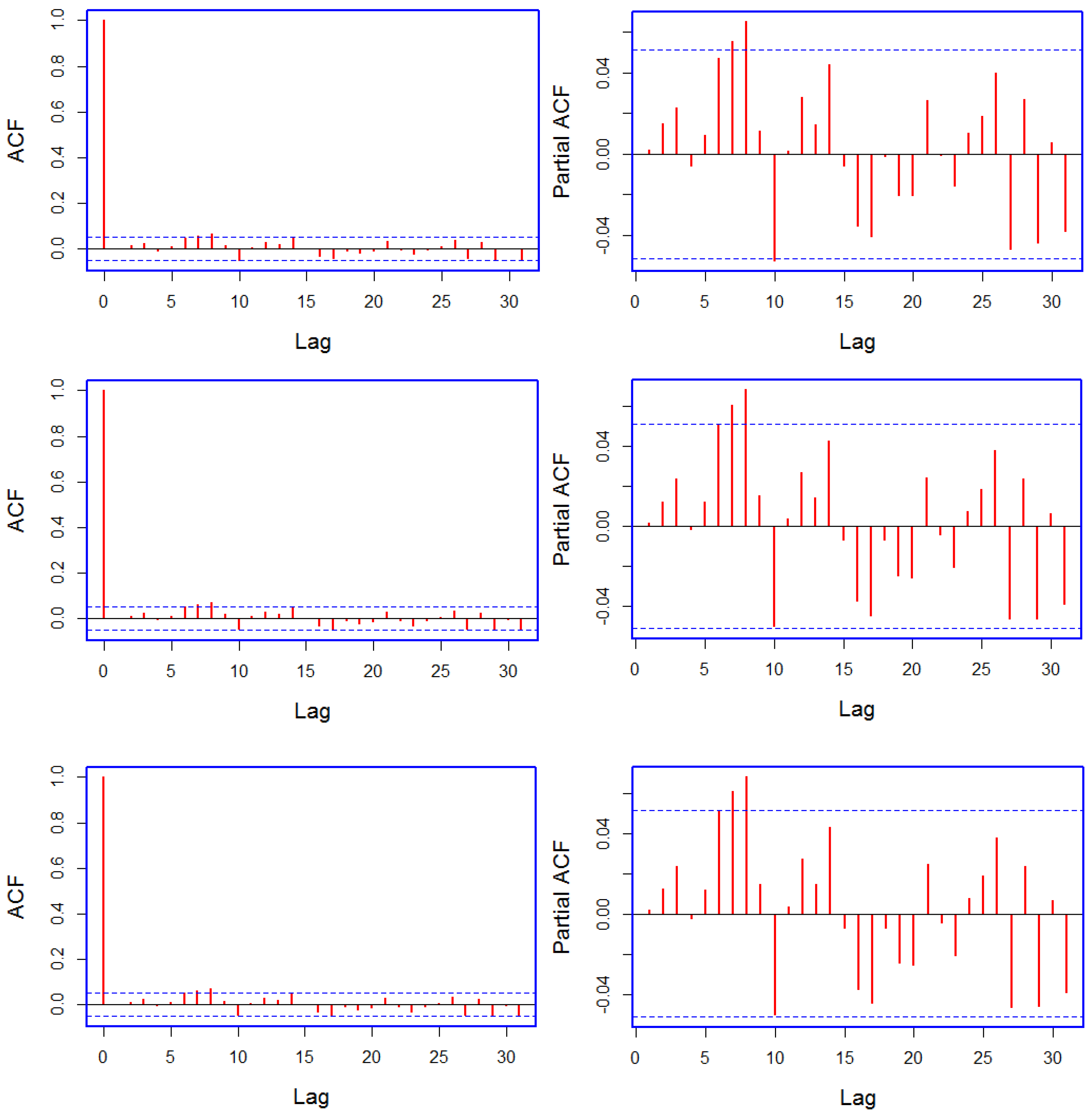
For the stochastic component $R_{t,j}$ and the final model error ${ϵ}_{t,j}$, examples of the Autocorrelation Function (ACF) and Partial Autocorrelation Function (PACF) are plotted in Figure 3 and Figure 4. Note that in the case of ${ϵ}_{t,j}$, both ACF and PACF refer to the models when VAR is used as a stochastic model. The reason for plotting the residual obtained after applying the VAR model to $R_{t,j}$ is the superior forecasting performance of the multivariate model (see

Table 1. Descriptive statistics for one-day-ahead out-of-sample forecasting: The column represents the estimation of the yearly component through Sinusoidal Regression (SR), Local regression (L1), Local regression (L2), Local regression (L3), Regression Spline (RS), and Smoothing Spline (SS). The row represents the estimation of the stochastic component thorough Autoregressive (AR), Non-Parametric Autoregressive (NPAR), Autoregressive Moving Average (ARMA), and Vector Autoregressive (VAR).

ERRORS	MODELS	SR	L1	L2	L3	RS	SS
MAPE	AR	2.503	2.466	2.413	2.412	2.411	2.412
	NPAR	2.510	2.434	2.413	2.411	2.399	2.395
	ARMA	2.514	2.435	2.413	2.418	2.405	2.396
	VAR	2.143	2.109	1.997	1.995	1.994	1.995
MAE	AR	1081.184	1069.125	1044.341	1044.686	1044.177	1044.611
	NPAR	1086.336	1056.392	1045.753	1046.899	1041.275	1039.804
	ARMA	1084.869	1055.017	1048.107	1045.881	1042.705	1038.553
	VAR	922.405	907.187	856.497	856.135	856.082	856.088
RMSE	AR	1486.580	1493.652	1450.551	1454.510	1450.676	1453.358
	NPAR	1476.394	1450.813	1436.108	1439.677	1434.670	1433.172
	ARMA	1468.908	1443.367	1431.686	1431.296	1427.437	1422.794
	VAR	1219.608	1211.225	1146.302	1146.002	1145.979	1146.014

). Overall, the residuals ${ϵ}_{t,j}$ of each model have been whitened. In some cases, residuals still show some significant correlation, but with an absolute value so small that it is useless for prediction.

3. Out-of-Sample Forecasting

This work considers the electricity demand data for the Nord Pool electricity market. The data cover the period from 1 January 2013–31 December 2016 (35,064 hourly demand levels for 1461 days). A few missing observations in the load series were replaced by averages of the neighboring observations. The whole dataset was divided into two parts: 1 January 2013-31 December 2015 (26,280 data points, covering 1095 days) for model estimation and 1 January 2016–31 December 2016 (8784 data points, covering 366 days) for one-day-ahead out-of-sample forecasting.

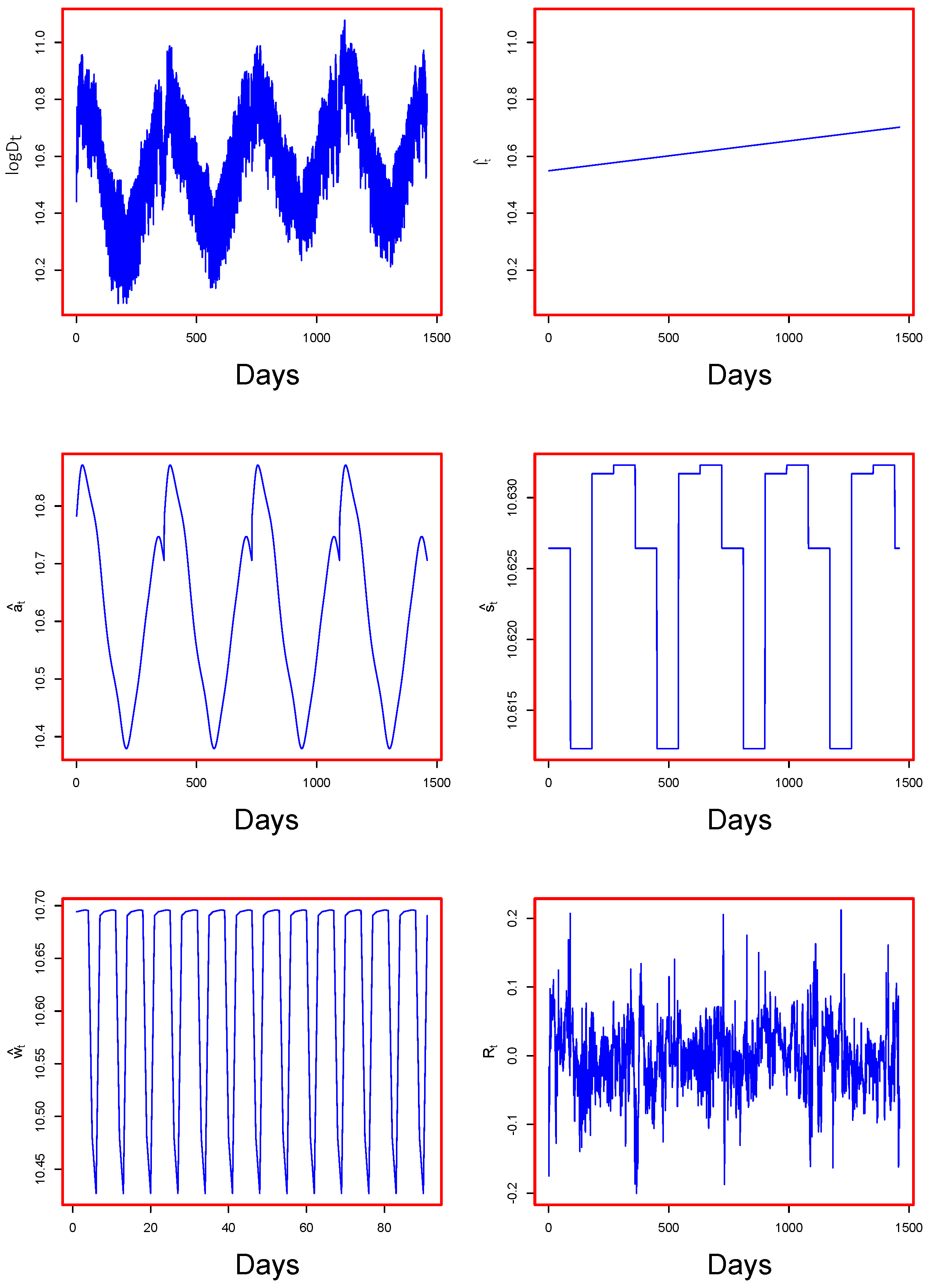
In the first step, the deterministic component was estimated separately for each load period as described in Section 2.1. An example of estimated deterministic components, as well as of $R_{t,j}$ is plotted in Figure 5. In the figure, along with the log demand at the top left, the long trend, yearly, seasonal, and weekly components are plotted on top right, middle left, middle right, and bottom left, respectively. Note that the elements of the deterministic components capture different dynamics of the log demand. An example of the series $R_{t,21}$ is plotted at the bottom right in Figure 5. In the second step, the previously-defined models for stochastic component were applied to the residual series $R_{t,j}$. In both steps, models were estimated and one-day-ahead forecasts were obtained for 366 days using the rolling window technique. Final demand forecasts were obtained using Equation (12).

To evaluate the forecasting performance of the final models obtained from different combinations of deterministic and stochastic components, three accuracy measures, namely Mean Absolute Percentage Error (MAPE), Mean Absolute Error (MAE), and Root Mean Squared Error (RMSE) were computed as:

$$\mathrm{MAPE}=\mathrm{mean}\left(\frac{|D_{t,j}-{\widehat{D}}_{t,j}|}{D_{t,j}}\right)\times 100$$

$$\mathrm{MAE}=\mathrm{mean}\left(|D_{t,j}-{\widehat{D}}_{t,j}|\right)$$

$$\mathrm{RMSE}=\sqrt{\mathrm{mean}{(D_{t,j}-{\widehat{D}}_{t,j})}^2},$$

where $D_{t,j}$ and ${\widehat{D}}_{t,j}$ are the observed and the forecasted demand for the $t^{\mathrm{th}}$ day (t = 1, 2, …, 366) and the $j^{\mathrm{th}}$$(j=1,2,\dots ,24)$ load period.

As within the deterministic component, this work used six different estimation methods for $a_{t,j}$, whereas the estimation of other elements was the same; six different combinations were obtained. On the other hand, four different models were used to model the stochastic component. Hence, the estimation of both, deterministic and stochastic, components led us to compare twenty four different models. For these twenty four models, one-day-ahead out-of-sample forecast results are listed in Table 1. 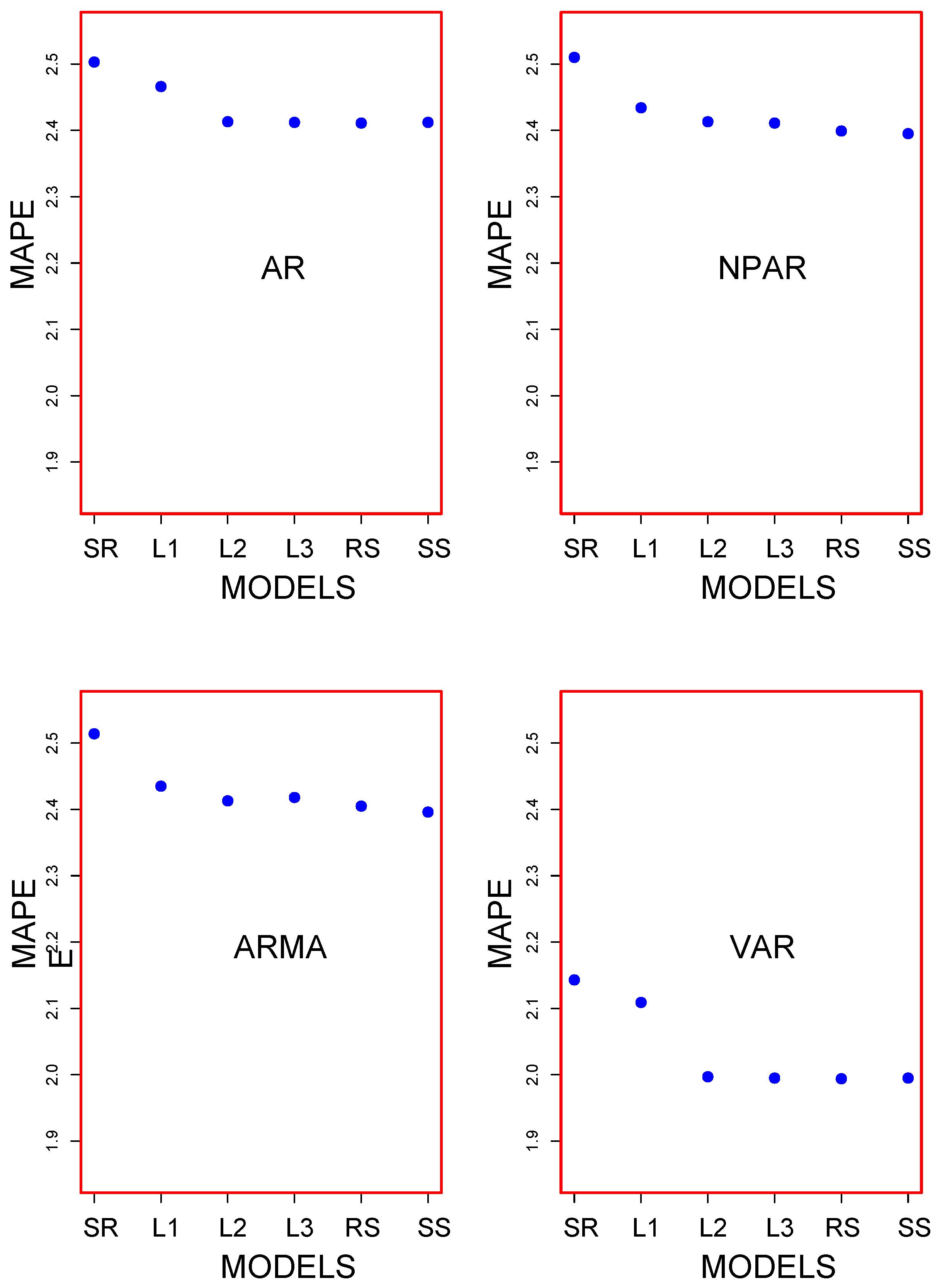From the table, it is evident that the multivariate VAR model combined with any estimation technique used for $a_{t,j}$ led to a better forecast compared to the univariate models. The best forecasting model was obtained by combining VAR and RS, which produced 1.994, 856.082, and 1145.979 for MAPE, MAE, and RMSE, respectively. VAR combined with SS or with L3 produced the second best results. Within the univariate models, NPAR combined with the spline-based regression models performed better than the other two parametric counterparts. Finally, any stochastic model combined with SR or with L1 led to the worst forecast in their respective classes (univariate and multivariate). Considering only MAPE, a graphical representation of the results for the twenty four combination is given in Figure 6. From the figure, we can easily see that multivariate models performed better than the univariate models. To assess the significance of the difference among accuracy measures listed in Table 1 for different combinations, we performed the Diebold and Mariano (DM) [50] test of equal forecast accuracy. The DM test is a widely-used statistical test for comparing forecasts obtained from different models. To understand it, consider two forecasts, ${\widehat{y}}_{1t}$ and ${\widehat{y}}_{2t}$, that are available for the time series $y_t$ for $t=1,\cdots ,T$. The associated forecast errors are ${ϵ}_{1t}=y_t-{\widehat{y}}_{1t}$ and ${ϵ}_{2t}=y_t-{\widehat{y}}_{2t}$. Let the loss associated with forecast error ${\left\{{ϵ}_{it}\right\}}_{i=1}^2$ by $L\left({ϵ}_{it}\right)$. For example, time t absolute loss would be $L\left({ϵ}_{it}\right)=\left|{ϵ}_{it}\right|$. The loss differential between Forecasts 1 and 2 for time t is then ${\eta }_t=L\left({ϵ}_{1t}\right)-L\left({ϵ}_{2t}\right)$. The null hypothesis of equal forecast accuracy for two forecast is $E\left[{\eta }_t\right]=0$. The DM test requires that the loss differential be covariance stationary, i.e.,

$$\begin{array}{ccc}\hfill E\left[{\eta }_t\right]& =& \mu ,\forall t\hfill \\ \hfill \mathrm{cov}({\eta }_t-{\eta }_{t-\tau })& =& \gamma \left(\tau \right),\forall t\hfill \\ \hfill \mathrm{var}\left({\eta }_t\right)& =& {\sigma }_{\eta },0<{\sigma }_{\eta }<\infty \hfill \end{array}$$

Under these assumptions, the DM test of equal forecast accuracy is:

$$\mathrm{DM}=\frac{\overline{\eta }}{{\widehat{\sigma }}_{\overline{\eta }}}\stackrel{d}{\to }N(0,1)$$

where $\overline{\eta }=\frac{1}{T}{\sum }_{t=1}^T{\eta }_t$ is the sample mean loss differential and ${\widehat{\sigma }}_{\overline{\eta }}$ is a consistent standard error estimate of ${\eta }_t$.

The results for the DM test are listed in

Table 2. p-values for the Diebold and Mariano test. $H_0$: the forecasting accuracy for the model in the row and the model in the column is the same; $H_1$: the forecasting accuracy of the model in the column is greater than that of the model in the row.

MODELS	RS-AR	RS-NPAR	RS-ARMA	RS-VAR
RS-AR	-	0.33	0.40	$<0.01$
RS-NPAR	0.67	-	0.75	$<0.01$
RS-ARMA	0.60	0.25	-	$<0.01$
RS-VAR	0.99	0.99	0.99	-

and

Table 3. p-values for the Diebold and Mariano test. $H_0$: the forecasting accuracy for the model in the row and the model in the column is the same; $H_1$: the forecasting accuracy of the model in the column is greater than that of the model in the row.

Models	SR-VAR	L1-VAR	L2-VAR	L3-VAR	RS-VAR	SS-VAR
SR-VAR	-	0.28	$<0.01$	$<0.01$	$<0.01$	$<0.01$
L1-VAR	0.72	-	$<0.01$	$<0.01$	0.01	$<0.01$
L2-VAR	0.99	0.99	-	0.93	0.85	0.83
L3-VAR	0.99	0.99	0.07	-	0.47	0.45
RS-VAR	0.99	0.99	0.15	0.53	-	0.48
SS-VAR	0.99	0.99	0.17	0.55	0.52	-

. The elements of these tables are p-values of the Diebold and Mariano test where the null hypothesis assumes no difference in the accuracy of predictors in the column and row against the alternative hypothesis that the predictor in the column is more accurate than the predictor in the row. From Table 2, it is clear that the multivariate VAR models outperform their univariate counterparts. When looking at the results of VAR using different methods of estimation for $a_{t,j}$ in Table 3, it can be seen that, except for SR-VAR and L1-VAR, the remaining four combinations had the same predictive ability. In the case of SR-VAR and L1-VAR, the remaining four combinations performed statistically better.

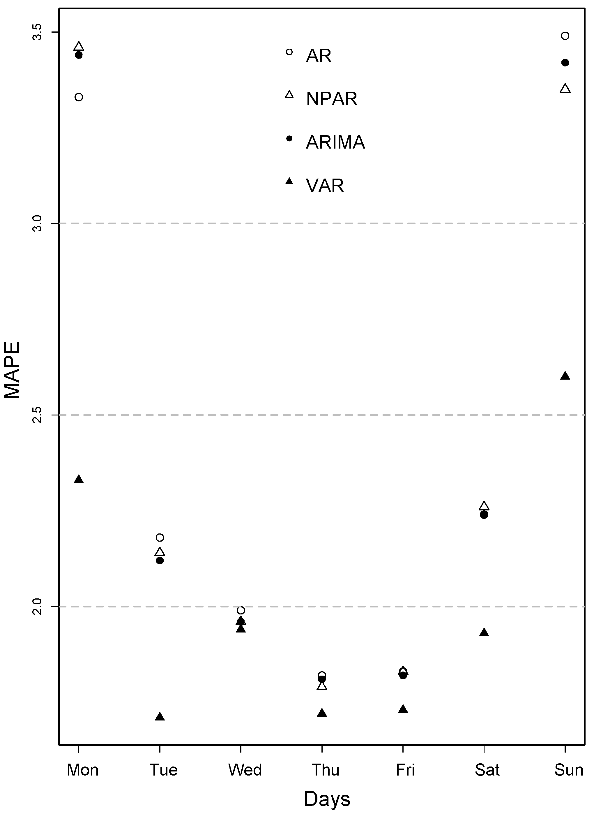
The day-specific MAPE, MAE, and RMSE are tabulated in

Table 4. Electricity demand: hourly day-specific MAPE, MAE, and RMSE.

ERRORS	MODELS	Monday	Tuesday	Wednesday	Thursday	Friday	Saturday	Sunday
MAPE	AR	3.33	2.18	1.99	1.82	1.83	2.24	3.49
	NPAR	3.46	2.14	1.96	1.79	1.83	2.26	3.35
	ARMA	3.44	2.12	1.96	1.81	1.82	2.24	3.42
	VAR	2.33	1.71	1.94	1.72	1.73	1.93	2.60
MAE	AR	1728.10	1002.69	755.78	633.24	634.54	905.95	1649.36
	NPAR	1811.31	973.38	740.55	618.19	638.20	921.64	1585.79
	ARMA	1798.48	969.16	743.45	626.00	631.97	912.87	1615.01
	VAR	1225.76	799.34	739.52	592.69	601.85	791.00	1250.86
RMSE	AR	2194.77	1288.65	980.01	774.78	798.23	1176.36	2142.07
	NPAR	2252.48	1253.27	950.24	764.92	795.33	1187.31	2038.49
	ARMA	2232.41	1248.31	952.02	775.92	789.30	1181.01	2028.24
	VAR	1601.44	999.26	963.13	733.99	747.15	981.53	1619.33

. From this table, we can see that day-specific MAPE was relatively higher on Monday and Sunday and smaller on other weekdays. As the VAR model performed better previously, the day-specific MAPE values for this model were considerably lower compared to univariate models, except on Wednesday, Thursday, and Friday. For these three days, both the univariate and multivariate models produced lower errors. The same findings can be seen by looking at day-specific MAE and day-specific RMSE. The day-specific MAPE values are also depicted in Figure 7. The figure clearly indicates that the MAPE value was lower in the middle of the week and was higher on Monday and Sunday.

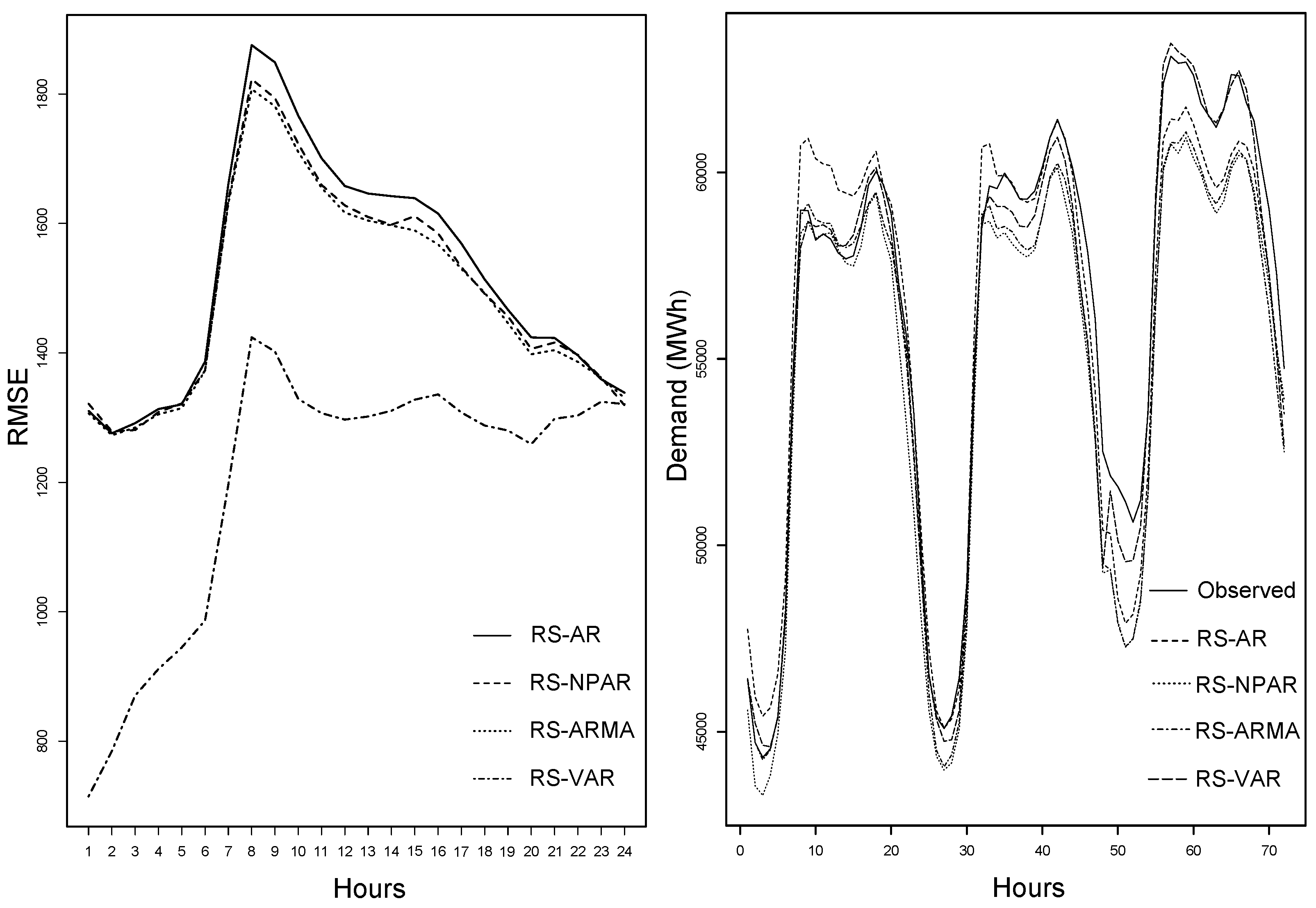
To conclude this section, the hourly RMSE and forecasted demand for the best four combinations including one for each stochastic model is plotted in Figure 8. From the figure (left), note that hourly RMSE are considerably lower at the low load periods, while they are high at peak load periods. Further, note the best forecasting performance of the SR-VAR model compared to the competing stochastic models. For these models, the observed and the forecasted demand are also plotted in Figure 8 (right). The forecasted demand was following the actual demand very well, especially when VAR was used as a stochastic model. Thus, we can conclude that the multivariate model VAR outperformed the univariate counterparts.

4. Conclusions

The main aim of this work was to model and forecast electricity demand using the component estimation method. For this purpose, the log demand was divided into two components: deterministic and stochastic. The elements of the deterministic component consisted of a long trend, multiple periodicities due to annual, seasonal, and weekly regular cycles, and bank holidays. Special attention was paid to the estimation of the yearly seasonality as it was previously ignored by many authors. The estimation of yearly components was based on six different estimation methods, whereas other elements of the deterministic component were estimated using ordinary least squares. In particular, for the estimation of annual periodicity, this work used the sinusoidal function-based model (SR), the local polynomial regression models with three different kernels: tri-cubic (L1), Gaussian (L2), and Epanechnikov (L3), Regression Splines (RS), and Smoothing Splines (SS). For the stochastic component, we used four univariate and multivariate models, namely the Autoregressive Model (AR), the Non-Parametric Autoregressive Model (NPAR), the Autoregressive Moving Average model (ARMA), and the Vector Autoregressive model (VAR). The estimation of both, deterministic and stochastic, components led us to compare twenty four different combinations of these models. To see the predictive performance of different models, demand data from the Nord Pool electricity market were used, and one-day-ahead out-of-sample forecasts were obtained for a complete year. The forecasting accuracy of the models was assessed through the MAPE, MAE, and RMSE. To assess the significance of the differences in the predictive performance of the models, the Diebold and Mariano test was performed. Results suggested that the component-wise estimation method was extremely effective for modeling and forecasting electricity demand. The best results were produced by combining RS and the VAR model, which led to the lowest error values. Further, all the combinations of the multivariate model VAR completely outperformed the univariate counterparts, suggesting the superiority of multivariate models. Within the combination of VAR, however, the results were not statistically different for all models.