A European Database of Building Energy Profiles to Support the Design of Ground Source Heat Pumps

Abstract

The design of ground source heat pumps is a fundamental step to ensure the high energy efficiency of heat pump systems throughout their operating years. To enhance the diffusion of ground source heat pump systems, two different tools are developed in the H2020 research project named, “Cheap GSHPs”: A design tool and a decision support system. In both cases, the energy demand of the buildings may not be calculated by the user. The main input data, to evaluate the size of the borehole heat exchangers, is the building energy demand. This paper presents a methodology to correlate energy demand, building typologies, and climatic conditions for different types of residential buildings. Rather than envelope properties, three insulation levels have been considered in different climatic conditions to set up a database of energy profiles. Analyzing European climatic test reference years, 23 locations have been considered. For each location, the overall energy and the mean hourly monthly energy profiles for heating and cooling have been calculated. Pre-calculated profiles are needed to size generation systems and, in particular, ground source heat pumps. For this reason, correlations based on the degree days for heating and cooling demand have been found in order to generalize the results for different buildings. These correlations depend on the Köppen–Geiger climate scale.

1. Introduction

The European Energy Efficiency Directive (2012/27/EU) demands the Member States (MS) to activate a suitable series of measures aimed toward a more efficient use of energy. Targets provided to every MS are being monitored in the period 2014–2020 to achieve the desired reduction of the total energy consumption, by means of a 20% decrease of energy efficiency improvements.

At worldwide level, the buildings sector accounts for about 31% of total global final energy use, 54% of final electricity demand, and 8% of energy-related CO₂ emissions (excluding indirect emissions due to electricity) [1]. In the European Union (EU) the energy consumption of buildings accounts for roughly 40% of the total final energy consumption and 36% of the European global CO₂ emissions [2]. The European Commission published the first directive, which aimed at improving the energy performance of buildings: The “Energy Performance of Buildings Directive” (EPBD) was introduced in 2002 [3]. Recast versions in 2010, and recently in 2018 [4,5], modified the previous versions, focusing on zero energy buildings (ZEB), HVAC (Heating Ventilating and Air Conditioning) systems, and renewable energy sources. Therefore, the way to reach the European objectives involves both the refurbishment of the European building stock, through a major renovation of the envelopes, and the diffusion of more efficient solutions for HVAC systems to increase renewable energy sharing.

When trying to enhance the efficiency of HVAC systems, ground source heat pumps (GSHPs) represent one of the most interesting renewable technologies. In the case of ordinary heat flow in soil, the temperature is usually almost constant below 7 m depth, reflecting the annual mean near-surface temperatures, as shown by Kusuda and Achenbach [6], who have mathematically modelled the annual sub-surface soil temperature based on the heat conduction theory applied to a semi-infinite homogenous medium. In general, the temperature in the Earth’s crust increases with depth: Down to depths of about 10,000 m, the average geothermal gradient is about 2–3 °C/100 m [7], which makes the ground a heat source or sink with constant temperatures through time.

The first patent on a ground source heat pump (GSHP) was developed by Zoelly in 1912 [8]. Since then, the installations of GSHP systems increased without interruption. The biggest benefit of GSHPs is that the amount of final and primary energy used is lower than conventional systems. The Department of Energy (DOE) and the Environmental Protection Agency (EPA) endorsed GSHP systems as among the most energy efficient and environmentally friendly heating, cooling, and water heating systems available [9]. GSHPs can provide energy for heating, cooling, and domestic hot water (DHW) production. Moreover, GSHPs, compared to air-source heat pumps, are less noisy, last longer, and need limited maintenance, and their energy efficiency does not depend on the temperature of the outside air. Nevertheless, their advantages are very often counteracted by the need of specialists to provide the design and characterization of the operating conditions in both the short- and long-term.

For promoting the diffusion of GSHPs and making the technology more accessible to the general public, in the research project, “Cheap and Efficient Application of Reliable Ground Source Heat Exchangers and Pumps” (Cheap-GSHPs), a tool for sizing these systems was developed, as well as a decision support system (DSS) able to assist the user in the preliminary design of the most suitable configuration. When the borehole heat exchangers coupled to the GSHP have to be sized, the overall energy demand of the building and the energy profiles for both heating and cooling conditions are the primary input data. There are different methodologies to design a GSHP: (a) The analytical models (e.g., the infinite line or cylindrical source model) [10,11,12], (b) the method based on the g-functions [13,14,15], and (c) numerical models (e.g., [16,17,18]). Depending on the methodology used, the heating/cooling energy demand of the building has to be provided by the following data:

• The monthly energy needs and the peak load for the infinite line source model;
• The monthly energy profiles for the transfer function method;
• The hourly thermal load profile for detailed models.

The borehole field cannot be sized only on the peak loads, like in other traditional systems, in order to avoid over- or under-sizing that involves both economic and technical disadvantages. The monthly energy loads of the building are very important in GSHP systems to investigate the long-term thermal behavior and the thermal drift of the ground temperature (i.e., the change of the ground temperature throughout the operating years) that affects the energy performance of the heat pump. The peak loads (in both heating and cooling) can be easily calculated by the user, since the calculation is simple (e.g., in heating mode, the calculation is based on the steady-state assumption). The calculation of the monthly energy loads requires additional work for the user. This work aims to fill this gap.

As already mentioned, in the Cheap-GSHPs project, two tools were developed; a design tool and a DSS, whose main objective is to help the designers, researchers, and stakeholders in the analysis of GSHPs. The tools share a common platform considering climatic conditions, building energy demand, thermal properties of the ground, strategies for the installation of heat pumps, and a renewable energy database to size GSHPs. Since the aims of the tools are different, there are different approaches.

Turban et al. (2005) generally define a DSS as: “A computer-based information system that combines models and data in attempt to solve semi-structured and some unstructured problems with extensive user involvement”. [19] The final aim of the DSS is to support the decision-making process, by providing the stakeholders at all the level with a series of scenarios. A DSS tool was developed within the Cheap-GSHPs project to accelerate the decision-making process of designers and building owners, as well as increase the market share of the Cheap-GSHP technologies. Different possible solutions are generated from the DSS, identifying the optimal solution within a defined general problem. Therefore, the user defines simple inputs (type of building, overall floor area or gross volume, and location) to generate a first cost-benefit analysis and to check if GSHPs can be installed or not. The DSS needs a consistent set of energy demand databases and simplified calculation methods to implement the different possible solutions, calculating the total length of the ground heat exchanger (GHE) field, according to the approach suggested by ASHRAE (American Society of Heating, Refrigerating and Air-Conditioning Engineers) [11,12], which is a proper design method. In fact, the outcome of the ASHRAE method is the total length of the borehole heat exchangers to satisfy the building thermal load. In other approaches, e.g., g-functions or numerical tools, the user has to set the total borehole length as well as the field layout and then simulate the plant-system, checking the temperatures of the heat-carried fluid and ground. For this reason, the ASHRAE approach can be useful, especially when the preliminary cost-benefit analyses have to be carried out.

Moreover, considering that the energy performance of buildings strictly depends on climatic conditions, and several attempts have been done to correlate energy demand and climatic indexes, this work tried to demonstrate that degree days can be an appropriate parameter to find simple correlations to calculate the building energy demand. This result can be very useful when a preliminary analysis (e.g., cost-benefit analysis) has to be carried out, especially with new heating-cooling systems, such as GSHPs. Nowadays, a detailed building load profile can be obtained via detailed models without highly computational resources, but, in this case, the user has to know many details about the building, such as, heat-gains, plant-systems, user behaviours, and schedules. All these input values are not easily known in a preliminary phase when important decisions are taken. To this purpose, this work looks at the calculation of the energy demand limiting the information requested of the user. In this analysis, the values of the degree days have been calculated based on Test Reference Year (TRY) from the Meteonorm [20] and EnergyPlus database [21] of the considered locations. Therefore, correlations are based on statistic data and are useful to obtain a preliminary evaluation of the heating and cooling energy demand of the building in a specific climate zone. These profiles can also be used when a comparison between sites with different climatic conditions have to be carried out.

On the other hand, the design tool is mainly addressed to designers. The calculation may be carried out in two ways: With a simplified method based on the ASHRAE approach [11,12] or with a detailed calculation based on the numerical tool CaRM (Capacitance Resistance Model) [16]. The designer has two main options: Building energy needs for heating/cooling are either known (hence the user aims to size the system) or might not be known (hence the user wants to make a first analysis) and, hence, have to be provided by a suitable database of building energy needs.

To meet the needs of both the DSS and the design tool, this work presents the set-up of the database, which collects the monthly average daily energy profiles of a selection of building types in different climatic conditions. Buildings representing some European residential typologies have been considered and modelled according to different insulation levels of the envelope. As similar approaches were not found in literature, a detailed analysis was carried out; the steps of the research are reported in the next sections.

2. Overview on Energy Modelling of Residential Building Stock

Works in literature have focussed so far on the possible energy savings in existing stock buildings. As an example, Sandberg et al. [22] explored the historical changes of the Norwegian dwelling stock, evaluating the improvements in energy efficiency and the consequent energy savings. The results of the model provided suitable explanations of the issues related to the evolution of the energy demand and the consequent energy saving solutions. Another work with similar philosophy was written by Swan et al. [23], who presented a model which investigates the influence of new technologies used in the Canadian housing stock. Statistical and heat mass transfer analyses have been used to study the energy use and predict the advantages related to the new technologies.

Other works in literature have tried to define building classifications. Schüler et al. [24] implemented a multi linear regression model to predict the annual heat demands of buildings within the canton of Geneva, developing eight building categories representative of 47,000 buildings. A work that shows some similarities to the present paper is the EU project, TABULA-EPISCOPE [25], where a database of building typical consumptions has been set up. EPISCOPE provides a huge amount of combinations of residential buildings and HVAC systems, including Nearly Zero Energy Buildings (NZEBs). The database provides the energy performance assessment before and after renovation, accounting actions both on the envelope and on the air-conditioning system. The TABULA-EPISCOPE project is based on National criteria, according to the building and plant features and weather conditions. The results are the overall consumptions of the buildings, while the present work aims at providing the average hourly profiles of the energy demands of the buildings. The results of the TABULA-EPISCOPE project may be used as input for the CHEAP-GSHP tools, but it has been necessary to set the hourly energy demand profiles.

Another work which may be also related to the current paper is the European project, iNSPiRe [26], whose goal is the development of a support tool that enables to predict the energy impact of different building retrofit solutions. iNSPiRe uses the TABULA building database to carry out an energy performance assessment, accounting several system typologies in seven European locations. The iNSPiRe report focuses mainly on the generation of systematic and modular renovation packages that can be applied directly on the building, reaching different target heating demand levels.

An interesting work has been presented by Huang and Broderick [27], who developed an engineering model to evaluate the contributions of the building elements to the heating and cooling loads, considering the “prototypical” residential dwelling of the American building stock in different climatic regions. Besides the fact that these simulations are based on US climate conditions, only the average characteristics of buildings’ have been considered and the proposed analysis cannot be fully implemented within European countries.

In this work, the idea is to consider four types of residential buildings, which represent the general archetypes in Europe, as shown in detail. Different climatic zones, according to the Köppen–Geiger Classification, have also been considered, selecting 23 European locations. More details on the analysis on climates carried out in the present project can be found in [28]. Respect to iNSPiRe, the four building typologies have been modelled in detail and evaluated by means of dynamic hourly simulations in the defined locations. Finally, the simulation results have been post-processed to provide reliable correlations to predict the building heating-cooling energy demand as a function of the typology, dimension, and climate.

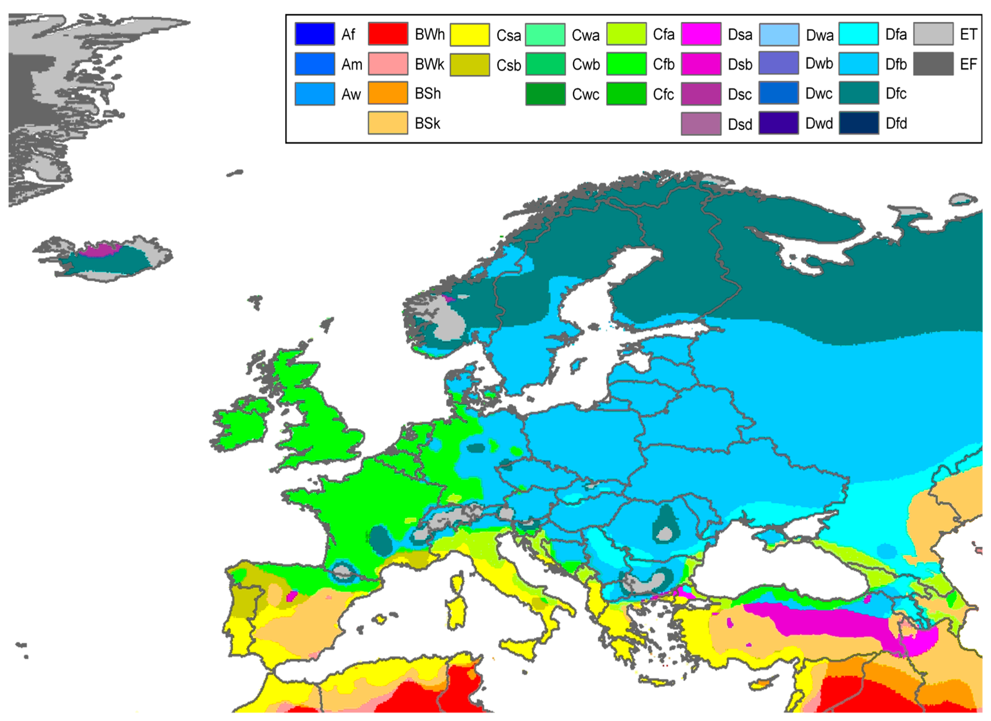
3. Climate Classification Analysis

Climate is a key factor when building energy needs are evaluated [29]. Hence, proper boundary conditions must be defined in terms of parameters affecting energy in buildings, which may be different from case to case, depending on the issue. In this work, attention has been paid to the ambient air and how to clearly define the climate.

Atmospheric temperature is governed by many factors, e.g., solar radiation, humidity, wind, and altitude. The annual atmospheric temperature range at any geographical location depends largely upon the type of ecosystem, as measured by the Köppen climate classification, which has been recently updated [30]. At present, climatic data is available for most of the climates; according to the present analysis, the test reference year came from several open source databases [31], with the only exception of Zurich, whose TRY belongs of the Meteonorm database [20]. Among the different ways to define the weather conditions, the Köppen–Geiger scale and the degree days (DDs) have been used [28]. The European map of the Köppen–Geiger climate classification is shown in Figure 1.

The Cheap-GSHPs project is focused on the geographical area of Europe. For this reason, TRYs from Europe have been collected in a climatic database [28]. Based on this analysis, 23 locations have been selected in 14 countries to represent the four climate classes, which are the most diffuse around Europe.

Table 1. List of the considered locations with geographical coordinates and the Köppen–Geiger Climate Classification.

Location	Coordinates	Climate Class	Location	Coordinates	Climate Class
Madrid (ES)	40.4° N–3.7° W	Csa	Bruxelles (BE)	50.9° N–4.4° E	Cfb
Athens (GR)	38.0° N–23.7° E	Csa	Zurich (CH)	47.4° N–8.6° E	Cfb
Cordoba (ES)	37.9° N–4.8° W	Csa	Berlin (DE)	52.5° N–13.4° E	Cfb
Palermo (IT)	38.1° N–13.4° E	Csa	London (GB)	51.5° N–0.1° W	Cfb
Lecce (IT)	40.4° N–18.2° E	Csa	Munich (DE)	48.1° N–11.6° E	Cfb
Coimbra (ES)	40.3° N–8.5° W	Csb	Lodz (PL)	51.8° N–19.5° E	Cfb
LaCoruna (ES)	42.4° N–8.4° W	Csb	Paris (FR)	48.9° N–2.4° W	Cfb
Bilbao (ES)	43.3° N–2.9° W	Csb	Helsinki (FI)	60.2° N–24.9° E	Dfb
Venice (IT)	45.4° N–12.3° E	Cfa	Minsk (BY)	53.9° N–27.5° E	Dfb
Milan (IT)	45.5° N–9.2° E	Cfa	Kaunas (LT)	54.9° N–23.9° E	Dfb
Bologna (IT)	44.5° N–11.3° E	Cfa	Debrecen (HU)	47.5° N–21.6° E	Dfb
Dublin (IE)	53.3° N–6.3° W	Cfb	-	-	-

reports the locations considered for the detailed analyses, according to their geographical coordinates and the relative Köppen–Geiger classification. This choice is in agreement with a similar work [33], where the authors considered a reference office room in Europe and analysed the heating and cooling energy demand. Although their approach was only based on the amount of heating and cooling degree days (HDDs and CDDs), its application lead to a classification with significant similarities with the maps produced on the basis of the Köppen–Geiger climate classification.

As already mentioned, besides the Köppen–Geiger scale, DDs have also been considered. DDs are essentially a simplified representation of outside air temperatures. They are widely used when the building energy demand is evaluated. HDDs are a measure of how much (in degrees), and for how long (in days), outside air temperature is lower than a specific base temperature or balance point. HDDs are often used for calculations relating to the building heating energy demand. In the present study, the reference period from 15 to 14 April has been considered as the heating season.

Similarly, CDDs are a measure of how much (in degrees), and for how long (in days), outside air temperature was higher than a specific base temperature. The corresponding cooling period can be identified between 15 April and 14 October to cover all the considered locations. The same approach used to calculate the HDDs and CDDs was set for each location, in order to find the common correlations between the energy demands and DDs.

As shown by Amico et al. [34] for Italian locations and Al-Hadhrami [35] over Saudi Arabia, the heating/cooling energy demands of a given building typology, with certain properties of the envelope, in a specific location in a simplified approach, may be considered directly proportional to the values of the HDD/CDD of that location. The calculation of HDDs/CDDs can also be used as a first check to understand if a location requires mostly heating or cooling energy or both, or to compare energy needs in different climate conditions.

HDDs are defined relatively to a base temperature, i.e., when the outside air temperature is higher than that inside and the building does not need heating. The appropriate value of the base temperature depends on the heating temperature of the building, which is related to the building’s characteristics and use as well as the internal gains [36]. The method mostly used to calculate an appropriate base temperature assumes to subtract the effect of the average internal heat gain from the building temperature, lowering the baseline temperature respect to the internal set point. This procedure introduces a sensible approximation. Furthermore, different buildings are generally heated at different set-point temperatures and internal heat gains change greatly from building to building.

Properly assessing the baseline temperature is the key to reducing the approximation introduced by a correlation between the energy demand and DDs. However, it is not simple to generalize this result to a series of buildings, even when they have common characteristics, the same use, similar management of HVAC systems, and similar internal gains. For this reason, in the present analysis, the baseline temperature (T_b) has been set for both heating and cooling conditions equal to 18 °C, and a threshold for the external temperature (T_t) was set, equal to 14 °C in HDD calculation and equal to 20 °C for the CDD evaluation. Considering that the buildings are managed under the same indoor set-point temperatures and that the same conditions concerning ventilation and internal gains have been considered in the calculations, the variation of the baseline temperature for the case studies would mainly depend on the envelope characteristics (thermal capacitance and U-value). However, the approximation introduced was found to be acceptable. To obtain a generic set of correlations between the energy performance of buildings in Europe and DDs, for each one of the 23 locations, a set of dynamic simulations were carried out to assess the heating and cooling energy demand of 4 types of buildings and different thermal insulation levels. Thus, a total number of 276 dynamic simulations were performed. The simulation was carried out through one year with an hourly calculation time step.

4. Building Selection and Dynamic Simulations

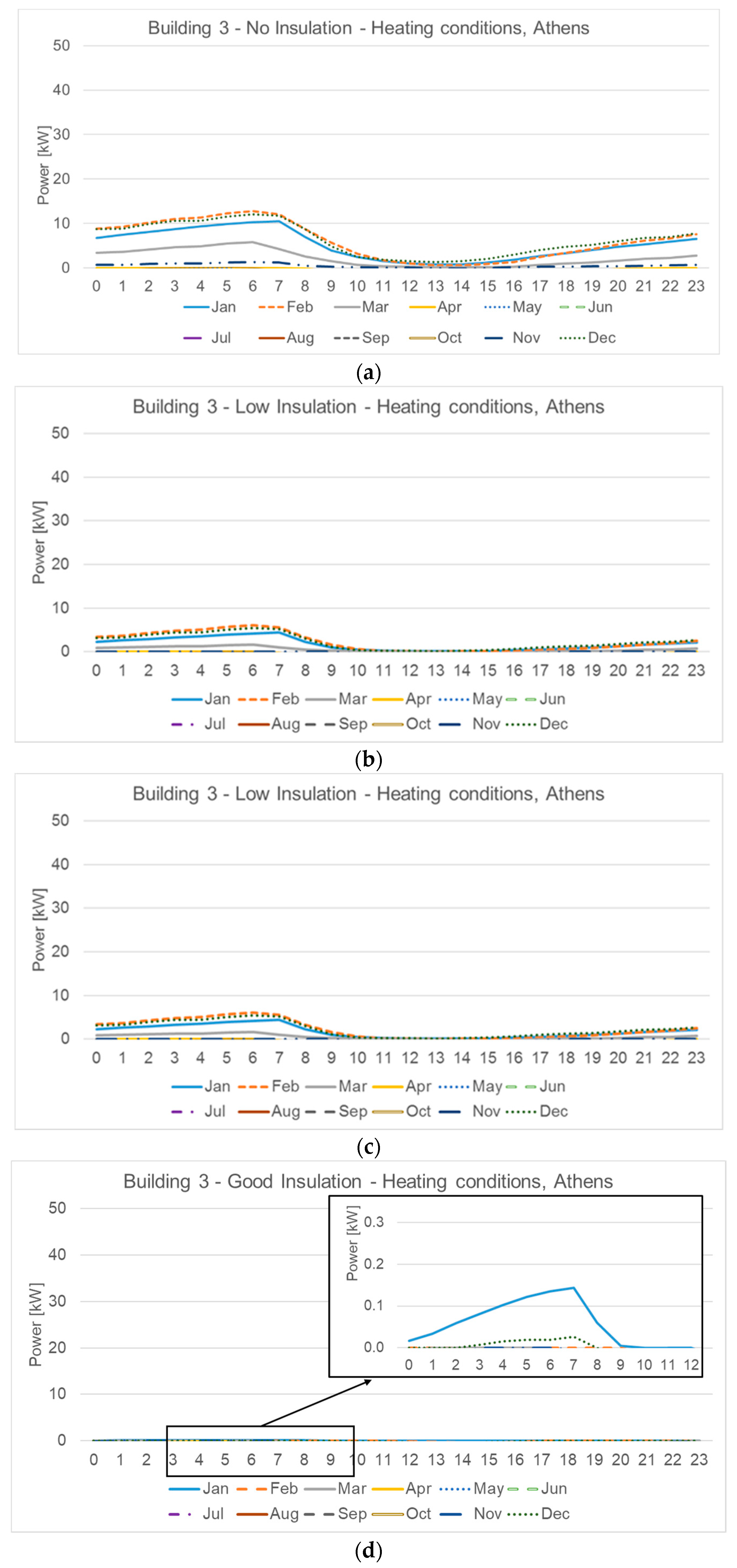
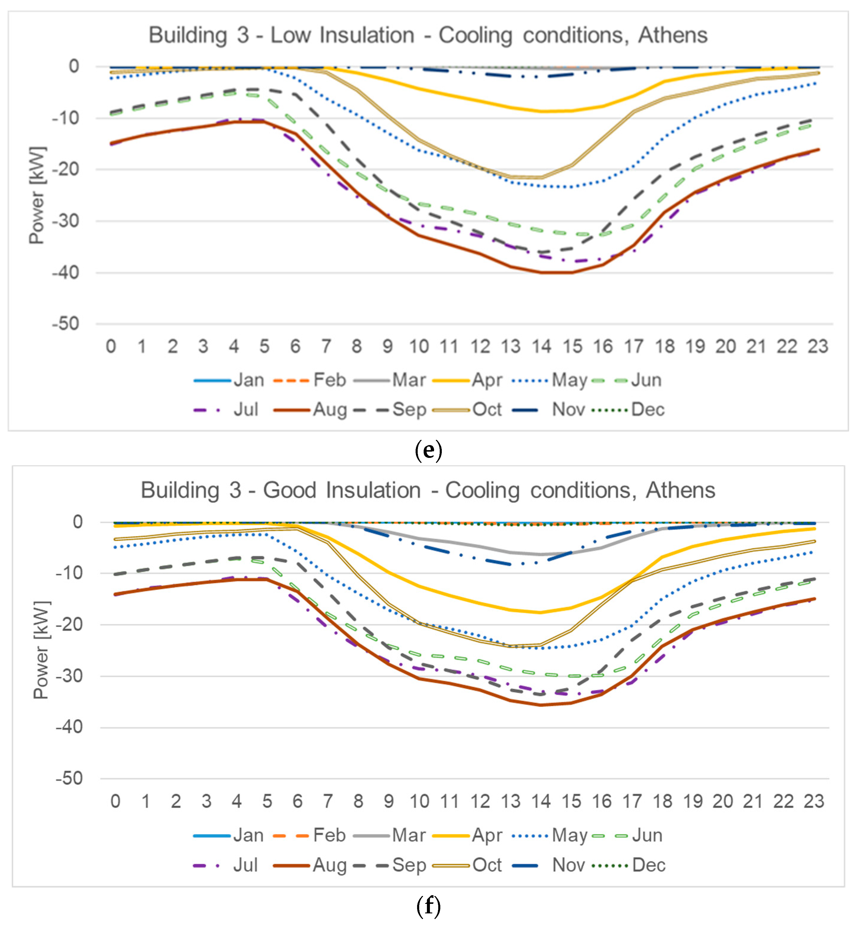
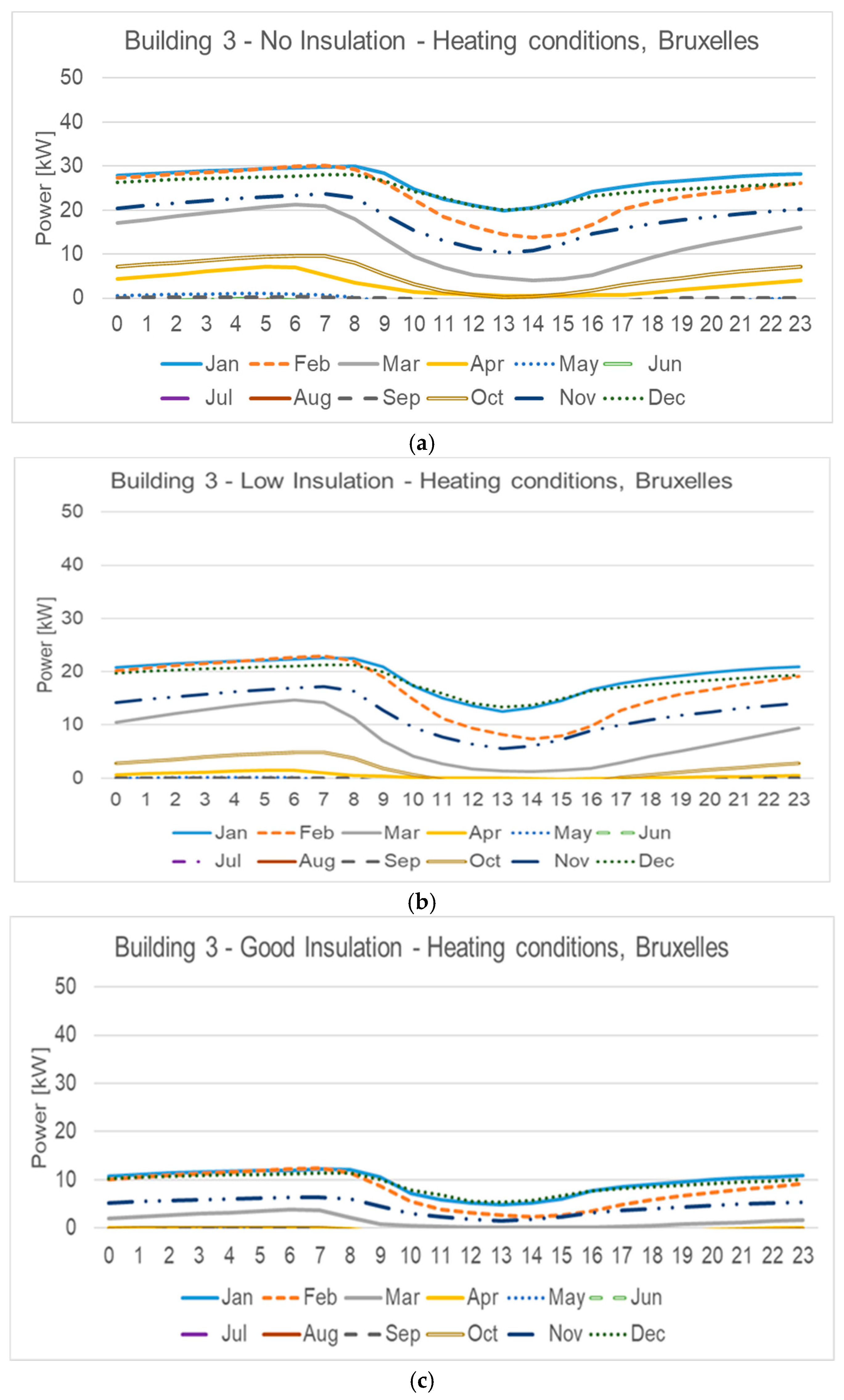
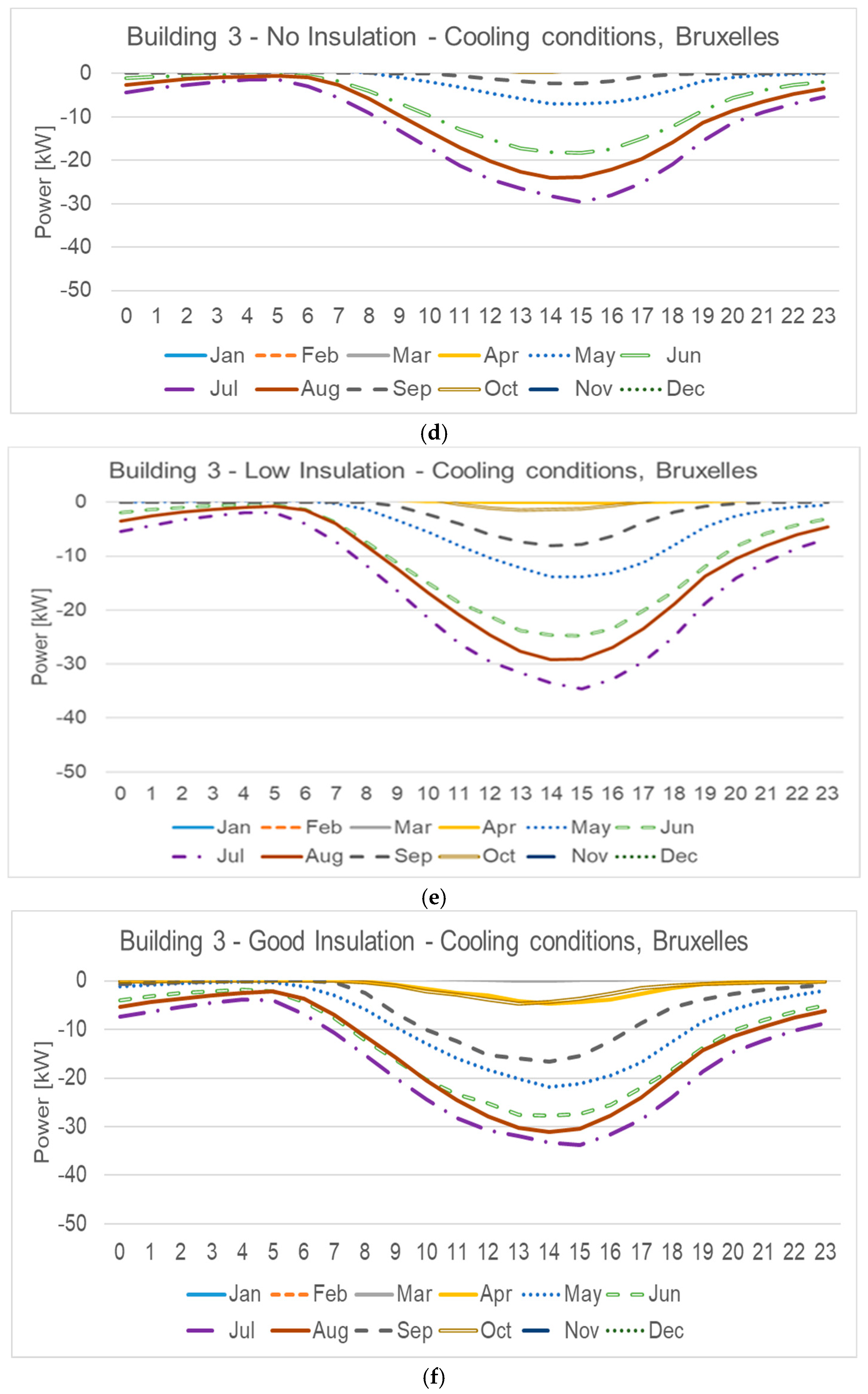
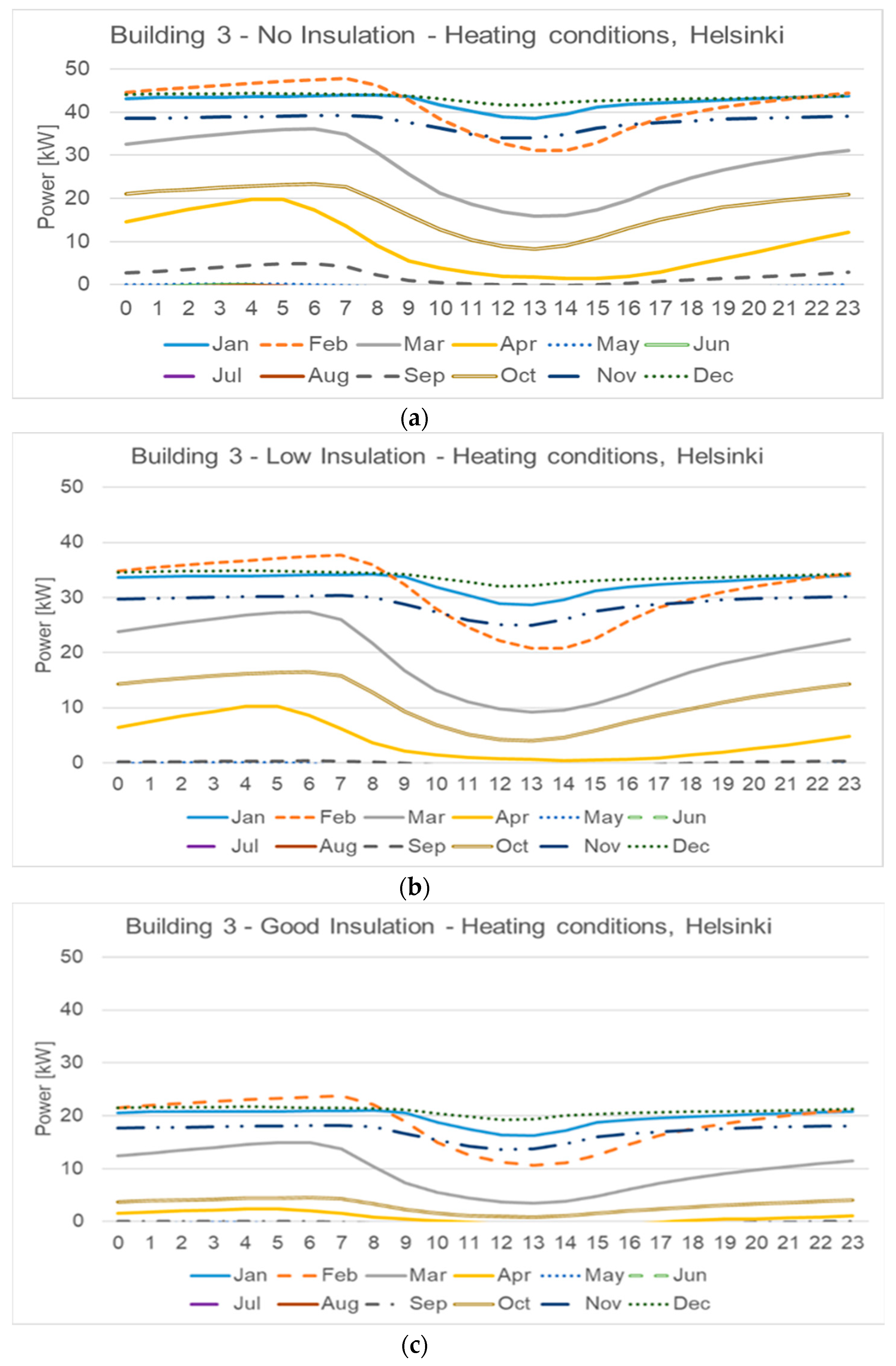
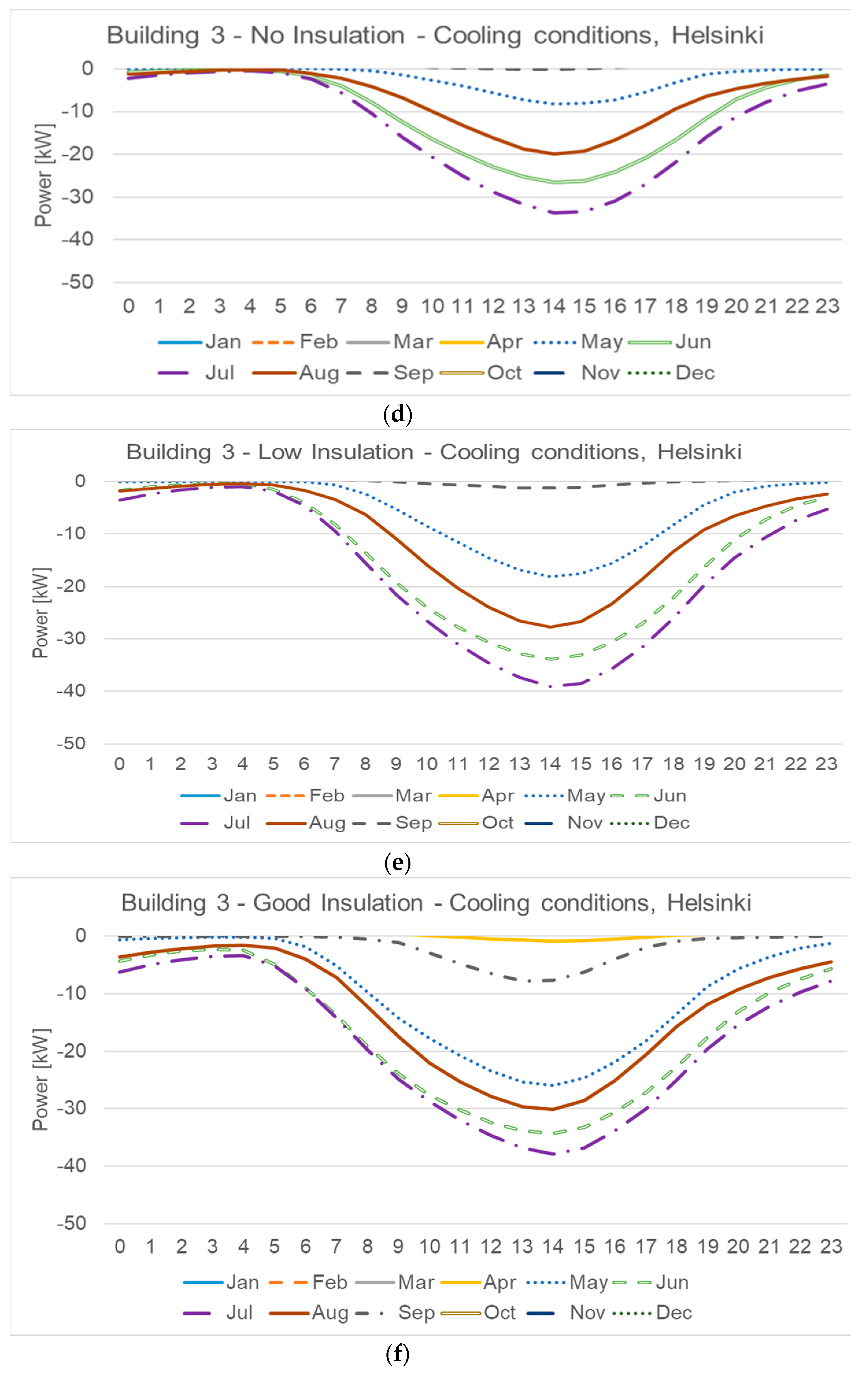
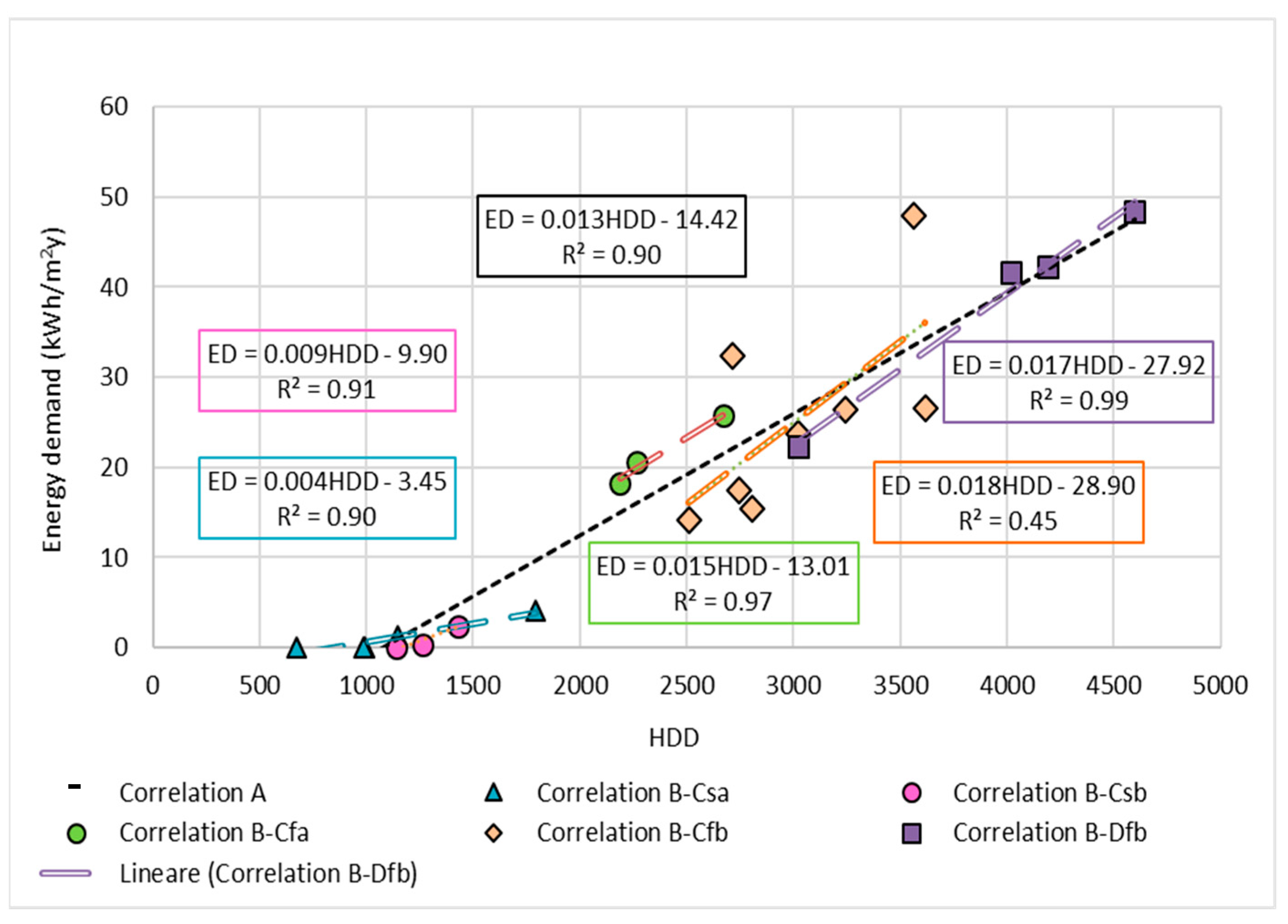
On the basis of statistical data concerning the state of buildings around Europe [37,38,39,40], this work analyzed four building categories as representative samples of the European residential building stock. Residential case studies, presented in

Table 2. General information for the investigated residential buildings.

Archetype Characteristics	Building 1	Building 2	Building 3	Building 4
External view
S/V ratio(m−1)	0.86	0.40	0.35	0.43
Net floor area Af (m2)	210	126	1330	681
Ag/Af (%)	14%	12%	25%	14%
No. of storeysover ground	2	3	5	5
No. of dwellings	1	1	20	10
Urban structure	stand alone	contiguous	stand alone	stand alone

, have been classified on the basis of the building category: Single house (Building 1 and Building 2) and terraced housing and apartment buildings (Building 3 and Building 4), considering both the surface, which dissipates heat and volume (S/V) ratio, and the glazed/floor area (A_g/A_f) ratio.

Each building has been modelled in a transient simulation environment using the software TRNSYS [41] to obtain the hourly energy demand for heating and cooling. Figure 2 outlines the model implemented in TRNSYS, which is mainly based on the Type 56 [41], which allows the simulation of the building. The ground floor of the building consists of a concrete slab where the ground temperature, calculated via the Type 77 of TRNSYS, has been applied as the boundary condition. The heating and cooling system has been modelled as an ideal convective system able to maintain the air temperature inside the dwelling equal to the set-point, which was 20 °C and 26 °C in heating and cooling, respectively; the relative humidity has been also controlled on 50%. Using TRNSYS for the borehole heat exchangers utilizes the approach proposed by Hellström [42], where the borehole length, the type of ground heat exchanger, and the thermal properties of the ground have to be set by the user; for this reason, only the building was simulated so that the borehole parameters could be set in the DSS by the user, according to the case-study investigated. The energy required for domestic hot water has been neglected because it depends mostly on the occupancy of the building and the low efficiency periods of the heat pumps should be avoided. Eventually, the energy profile of the DHW can be calculated separately and summed up at the thermal load profile of the building.

The envelope structures have been implemented in detail considering the thermo-physical properties of walls, roofs, floors, and windows, using typical values, according to the age and topology of the building. The envelope structure is based on common hollow bricks (U = 1.25 W/(m² K)) and hollow-core concrete roofs. This assumption was done to consider an average thermal capacitance of the structure and, as a consequence, to cover the building construction techniques used in several countries; as reported in [25], the hollow bricks and hollow-core concrete roofs are used in several European countries. A total of three thermal insulation levels were then: No insulation, low (i.e., 6 cm polystyrene) and good (i.e., 15 cm polystyrene) insulation levels. These average insulation levels, provided by the Italian Standards [43,44], developed in agreement with the EPBD package recast [3,4], have been decided to be installed in relatively new buildings or retrofitted in the last 10–15 years. As mentioned, the energy profiles obtained from the correlations will be used to make a rough sizing of the borehole field coupled to the GSHP systems. Consequently, the developed database is more focused on the building end use and typology rather than its structure, which is the reason why the analysis used a common envelope stratigraphy.

Regarding glazing surfaces, each typology has been characterized by standard properties. The property of glasses and frame were implemented on the basis of literature surveys. Existing windows usually do not satisfy current standard requirements, since single glazing windows are still largely used, and the U-value of average windows around Europe is about 2.5 W/(m² K) [45,46,47]. In the present analysis, the case studies without insulation and with low insulation level have double-glazed windows with an overall U-value of about 2.8 W/(m² K). The well insulated envelope was modelled with double-glazed windows with low emissivity, to guarantee an overall U-value equal to 1.4 W/(m² K). A 15% wooden frame surface is considered in each building. Shading devices were not considered for glazing surfaces, since their settings can change in each location according to the local weather.

Considering the noticeable effect that occupancy has on the thermal energy demand [48,49,50,51], internal gains, due to people and lighting systems, in agreement with the standard EN ISO 13790 [52], have been calculated according to the Italian Standard [53]. The sensible heat gain (φ_int) has been assumed, based on Equation (1):

$${\mathsf{\Phi }}_{\mathrm{int}}=7.987·{\mathrm{A}}_{\mathrm{f}}-0.0353 · {\mathrm{A}}_{\mathrm{f}}{}^2\left(\mathrm{W}\right)$$

(1)

where A_f is the net floor area of the building. In the case of dwellings with net floor areas greater than 120 m² for a single residential unit, the value of the heat gain has been set equal to 450 W. The contribution of the heat gains was considered 60% as convective rate and 40% as radiant rate.

Moreover, the effect of air infiltrations and natural ventilation on the heating and cooling energy demand have been considered using an average value of about 0.3 air change hour (ACH), as suggested by the Italian standard [53] and in agreement with some monitoring campaigns conducted on sample buildings in the past years [54]. The air infiltration rate was kept constant throughout the year. The same value (i.e., 0.3 ACH) can be assumed as realistic, even if a combination of 0.1 ACH of basic infiltration and 0.5 ACH of mechanical ventilation is considered, supposing that the mechanical ventilation systems is equipped with a 60% efficiency heat recovery. In exiting non-insulated buildings, the air infiltration rate could be higher than 0.3 ACH, but in this case, the GSHPs should be considered after the improvement of the building envelope. Open options to decrease the energy consumption of buildings include improving the quality of the envelopes in buildings’ and using energy-efficient heating and cooling technologies, based on renewable energies. As a matter of fact, the three thermal insulation levels were investigated in order to highlight the importance of optimizing the building envelope, considering the case study without insulation as a baseline to compare the two retrofit solutions.

For the single family houses models, the building was divided into only one thermal zone per floor, while, in Buildings 3 and 4, each flat was modelled as a single thermal zone. These assumptions were set in order to avoid having to consider the different schedules of users within the same dwelling, because these highly depend on the type of user, e.g., old people or young couples. As the objective of the computer simulations was to find the energy demand of the building, the same value of the set-point in each room of the dwelling was assumed to avoid the consideration of another variable in the analysis. One orientation has been considered for each building, fixing the main entrance facing South. An overall number of 276 dynamic simulations (4 building types × 3 levels of insulation × 23 climates) have been carried out. Annual simulations have been carried out with hourly time step via TRNSYS; the resulting hourly load profile for the average day of the month has been evaluated calculating the average value hour by hour. These profiles can be useful for the allocation of the monthly heating/cooling energy loads on an hourly based average day condition for sizing a ground source heat pump system.

As an example, some simulation results are shown in Figure 3, Figure 4 and Figure 5, where the heating and cooling energy profiles for the multifamily Building 3 are presented for Athens, Bruxelles, and Helsinki. The energy profiles are also shown taking into consideration the three thermal insulation levels, i.e., no insulation, low and good insulation.

Figure 3 outlines hourly profiles for heating and cooling of a typical apartment block in Athens. In particular, Figure 3a–c show the heating energy demand for no insulation, low and good insulation, respectively. Moving from no insulation (Figure 3a) to good insulation (Figure 3c), the average thermal power decreases by more than 95%. The HDD value (995) is lower than that of the other climates, and, consequently, the peak of the profiles is low. On the contrary, the maximum value of the cooling energy demand is about 40 kW for the case with no insulation (Figure 3d). As can be seen, when the thermal insulation level raises the cooling energy demand increases, especially for the first and last months of the cooling season, whereas the value corresponding to the design month (August in this case) slightly decreases. This thermal behaviour is due to the combination of the effects of internal gains, weather conditions, and thermal properties of the structures; this result can be observed in each location, even if it is more evident in Athens, due to the more severe weather conditions during the cooling season.

Bruxelles (Figure 4) has a higher HDD value (2747), hence, from the graph, a significant reduction of about 27% of the energy demand using 6 cm of polystyrene (i.e., low insulation) and up to 60% with 15 cm of polystyrene (i.e., good insulation) is evident. Although this strategy reduces heating energy demand, cooling energy demand increases by 16%, with respect to non-insulated buildings. This effect is more evident for the Helsinki climate (Figure 5); as the CDD value here is very low (27), there is less evidence of the increased cooling energy demand (up to 18%), while, for the heating conditions, the energy required is reduced by 50%.

Further considerations must be done for the cooling loads, which depend mostly on the solar radiation: For this reason, in order to help the reader, the average monthly weather data (i.e., external air temperature and global solar radiation) and the HDD and CDD values are shown for each location (

Table 3. Average monthly climatic data and energy demand of Athens.

Month	Jan.	Feb.	Mar.	Apr.	May	Jun.	Jul.	Aug.	Sep.	Oct.	Nov.	Dec.
Average T (°C)	10.70	9.58	11.39	15.06	19.61	24.61	27.30	27.59	23.88	19.15	14.51	10.86
Monthly Statistics Global Radiation (Wh/m2)	2068	2815	4012	5144	6215	7479	7529	6626	5421	3522	2141	1809
No Insulation (kWh)	3843	4123	1674	0	−5497	−12,759	−17,533	−17,871	−11,931	0	386	4740
Low Insulation (kWh)	1262	1500	394	0	−7555	−13,620	−17,702	−18,035	−13,113	0	1	1661
Good Insulation (kWh)	24	0	0	0	−9372	−13,388	−16,282	−16,527	−13,176	0	0	3
HDD (CDD)	995 (1052)

,

Table 4. Average monthly climatic data and energy demand of Bruxelles.

Month	Jan.	Feb.	Mar.	Apr.	May	Jun.	Jul.	Aug.	Sep.	Oct.	Nov.	Dec.
Average T (°C)	3.06	3.23	6.44	8.90	12.93	15.56	18.43	17.43	14.47	10.93	6.59	4.93
Monthly Statistics Global Radiation (Wh/m2)	659	1240	1931	3192	4334	4343	4705	4036	2613	1688	892	454
No insulation (kWh)	19,625	15,871	9636	2251	−1562	−5266	−9798	−7460	−333	3989	13,052	18,616
Low insulation (kWh)	14,192	11,129	5546	344	−3468	−7533	−11,864	−9215	−1485	1567	8792	13,636
Good Insulation (kWh)	7037	5191	1102	5	−6378	−9510	−12,880	−10,644	−4036	7	3175	6781
HDD (CDD)	2747 (72)

and

Table 5. Average monthly climatic data and energy demand of Helsinki.

Month	Jan.	Feb.	Mar.	Apr.	May	Jun.	Jul.	Aug.	Sep.	Oct.	Nov.	Dec.
Average T (°C)	−3.86	−5.67	−1.00	3.67	9.86	14.01	16.70	15.75	10.24	5.86	−1.26	−2.97
Monthly Statistics Global Radiation (Wh/m2)	250	910	1869	3576	5311	5744	5441	4017	2347	1124	314	119
No insulation (kWh)	31,596	27,744	20,164	6641	−1732	−7623	−10472	−5352	−43	12,948	27,154	32,302
Low insulation (kWh)	24,300	20,871	14,032	2942	−4331	−10,652	−13,044	−7767	−201	8273	20,753	25,194
Good insulation(kWh)	14,661	12,437	7019	671	−7601	−12,335	−14,111	−9851	−1351	2195	12,169	15,550
HDD (CDD)	4597 (17)

). In fact, each graph presents the hourly cooling load of the average monthly day, which can be misleading in comparison with different locations, if the solar radiation is not considered carefully. As can be seen, when the solar radiation reaches the maximum values, the cooling loads are comparable between the locations, but the profiles of other months are totally different. Table 3, Table 4 and Table 5 also summarize the monthly energy demand.

5. Results

Heating and cooling energy profiles have been analysed on a monthly and annual basis considering the building type (Building 1, Building 2, Building 3, and Building 4), the insulation level of the envelope (No Insulation, Low Insulation, Good Insulation), and climate.

These profiles can be used as representative of the building typologies considered to size the borehole field in a GSHP system. In fact, to implement the ASHRAE method [11,12], the energy demand of the building is required. As a matter of fact, when a first sizing of the GSHP is needed, the monthly profiles obtained can be used as standard profiles for the building typologies in the considered climate. In addition, the ratio between the annual heating and cooling energy demands (i.e., if the building’s annual load profile is balanced, heating, or cooling dominant) can be evaluated; this information affects the design of the borehole field. The same procedure is applied in the Cheap-GSHPs project to implement the design tool and decision support system.

Furthermore, the annual specific energy demand per floor area and the DD_y have been correlated using a simple linear regression. First, a correlation was found as a linear regression among all the locations; this correlation has been named “Correlation A”. A further analysis was then carried out, separately considering the locations in the same climate class; therefore, five additional correlations were obtained, one for each Köppen–Geiger climate class involved in the analysis: This method is referred as “Correlation B”.

The correlations have been evaluated for both heating and cooling conditions. An example (Building 3 with good insulation level) is provided in Figure 6 in the heating case. As can be seen, plotting the heating energy demand versus HDD, the general Correlation A may lead to negative values below a certain limit of HDD (in Figure 6 it is 1000 HDD), which can be considered a limited threshold value for the validity of the method.

The overall results for annual specific heating energy demands, ED_h in kWh/(m²·y), calculated using Equation (2), are reported in

Table 6. Correlations between HDD and heating energy demand for several residential buildings.

Type	Correlation ED = M × HDD + B		No Insulation					Low Insulation					Good Insulation
			M	B	R	R2	HDD limit	M	B	R	R2	HDD limit	M	B	R	R2	HDD limit
Building 1	General (A)		0.057	33.79	0.98	0.96	-	0.032	3.21	0.98	0.96	-	0.02	−4.69	0.98	0.96	-
	Köppen–Geiger (B)	Csa	0.055	30.54	0.97	0.94	-	0.028	4.45	0.95	0.91	-	0.016	−1.58	0.94	0.87	>100
		Csb	0.284	−241.55	0.97	0.95	-	0.120	−107.26	0.99	0.98		0.046	−41.12	1.00	1.00
		Cfa	0.061	41.57	1	1	-	0.033	11.97	1	1	-	0.02	2.33	1	1	-
		Cfb	0.059	27.25	0.87	0.75	-	0.033	−2.76	0.88	0.78	>100	0.021	−8.17	0.88	0.78	>400
		Dfb	0.061	12.84	0.97	0.94	-	0.035	−11.89	0.98	0.96	>350	0.023	−15.65	0.98	0.96	>680
Building 2	General (A)		0.042	5.54	0.99	0.98	-	0.022	−8.29	0.98	0.97	>22	0.015	−9.14	0.98	0.96	>615
	Köppen–Geiger (B)	Csa	0.039	7.1	0.98	0.95	-	0.017	−4.37	0.96	0.91	>255	0.011	−5.02	0.94	0.89	>470
		Csb	0.108	−77.01	0.99	0.98		0.045	−39.64	1.00	1.00		0.025	−24.00	1.00	0.99
		Cfa	0.041	18.96	1	1	-	0.022	−2.22	1	1	>100	0.015	−4.53	1	1	>300
		Cfb	0.041	8.23	0.94	0.89	-	0.023	−15.52	0.93	0.86	>670	0.016	−15.5	0.93	0.87	>950
		Dfb	0.047	−12.49	0.99	0.97	>270	0.025	−20.00	0.99	0.97	>810	0.018	−19.45	0.99	0.98	>1100
Building 3	General (A)		0.029	−14.82	0.98	0.96	>225	0.022	−16.19	0.97	0.94	>435	0.013	−13.33	0.93	0.87	>1015
	Köppen–Geiger (B)	Csa	0.021	−7.2	0.92	0.85	>345	0.014	−7.84	0.91	0.83	>580	0.004	−3.45	0.95	0.9	>850
		Csb	0.068	−66.05	1.00	1.00		0.043	−45.95	0.99	0.99		0.009	−9.90	0.96	0.91
		Cfa	0.032	−8.35	1	1	>265	0.024	−11.25	1	0.99	>465	0.015	−13.01	0.99	0.97	>895
		Cfb	0.033	−29.22	0.92	0.85	>885	0.025	−29.09	0.91	0.83	>1150	0.018	−28.9	0.67	0.45	>1610
		Dfb	0.033	−29.6	0.98	0.97	>895	0.026	−31.45	0.98	0.97	>1200	0.017	−27.92	0.99	0.99	>1660
Building 4	General (A)		0.038	0.6	0.97	0.94	-	0.022	−13.97	0.97	0.94	>630	0.012	−12.3	0.95	0.91	>1055
	Köppen–Geiger (B)	Csa	0.032	2.96	0.94	0.89	-	0.014	−6.54	0.88	0.78	>475	0.003	−2.83	0.94	0.88	>830
		Csb	0.172	−165.39	0.99	0.98		0.065	−70.34	1.00	1.00		0.011	−12.77	0.95	0.91
		Cfa	0.043	5.12	1	1	-	0.025	−9.29	1	1	>380	0.014	−11.81	0.99	0.99	>875
		Cfb	0.043	−17.29	0.86	0.74	>400	0.025	−24.06	0.87	0.76	>980	0.014	−23.29	0.9	0.8	>1635
		Dfb	0.042	−19.02	0.97	0.94	>455	0.026	−28.74	0.98	0.95	>1110	0.016	−26.48	0.99	0.98	>1675

, where columns M and B represent the slope and the intercept values of the linear regression, while R and R² are the residues and the quadratic residues of the correlations. In addition, the limit values of the DDs for the validity of the correlations are also reported to make easier their implementation.

ED_h = M × HDD + B

(2)

Using the same approach, the annual specific cooling energy demand ((ED_c) in kWh/(m²·y)) can be calculated by means of Equation (3), obtaining the results reported in

Table 7. Correlations between CDD and cooling energy demand for several residential buildings.

Type	Correlation ED = M × CDD + B		No Insulation					Low Insulation					Good Insulation
			M	B	R	R2	CDD limit	M	B	R	R2	CDD limit	M	B	R	R2	CDD limit
Building 1	General (A)		0.028	2.47	0.91	0.84	-	0.029	6.51	0.87	0.75	-	0.025	7.27	0.87	0.75	-
	Köppen–Geiger (B)	Csa	0.035	−3.01	0.94	0.88	>90	0.034	2.79	0.9	0.82	-	0.028	5.22	0.9	0.82	-
		Csb	0.037	−1.50	0.86	0.73		0.051	−0.13	0.80	0.64		0.039	2.93	0.77	0.59
		Cfa	0.033	−3.6	1	1	>110	0.031	0.63	0.99	0.98	-	0.023	3.82	0.98	0.96	-
		Cfb	0.048	1.14	0.64	0.41	-	0.064	3.83	0.53	0.28	-	0.06	4.62	0.53	0.28	-
		Dfb	0.087	−0.54	0.97	0.94	>10	0.098	3.2	0.93	0.86	-	0.081	4.54	0.92	0.84	-
Building 2	General (A)		0.036	4.64	0.91	0.83	-	0.035	15.43	0.83	0.7	-	0.031	17.92	0.83	0.69	-
	Köppen–Geiger (B)	Csa	0.042	0.85	0.84	0.7	-	0.04	12.55	0.8	0.65	-	0.035	15.98	0.82	0.67	-
		Csb	0.040	1.51	0.78	0.61		0.053	12.00	0.72	0.52		0.049	16.84	0.70	0.48
		Cfa	0.04	−2.25	0.98	0.97	>60	0.034	8.69	1	0.99	-	0.025	13.73	0.99	0.99	-
		Cfb	0.062	3.13	0.58	0.34	-	0.1	10.74	0.56	0.31	-	0.086	14.05	0.53	0.28	-
		Dfb	0.098	1.27	0.95	0.91	-	0.114	11.94	0.91	0.82	-	0.101	14.55	0.9	0.82	-
Building 3	General (A)		0.032	14.88	0.78	0.61	-	0.031	21.67	0.73	0.53	-	0.036	25.35	0.71	0.5	-
	Köppen–Geiger (B)	Csa	0.04	8.43	0.89	0.8	-	0.04	14.52	0.89	0.79	-	0.037	24.24	0.88	0.77	-
		Csb	0.060	5.05	0.81	0.66		0.067	11.83	0.79	0.62		0.065	24.33	0.72	0.52
		Cfa	0.042	4.96	0.99	0.99	-	0.04	11.45	1	0.99	-	0.032	21.16	0.99	0.99	-
		Cfb	0.111	8.68	0.53	0.28	-	0.123	14.45	0.5	0.25	-	0.177	12.63	0.51	0.26	-
		Dfb	0.13	10.59	0.89	0.79	-	0.137	17.26	0.87	0.75	-	0.127	24.82	0.86	0.73	-
Building 4	General (A)		0.015	8.46	0.58	0.34	-	0.019	15.67	0.61	0.38	-	0.022	24.11	0.68	0.46	-
	Köppen–Geiger (B)	Csa	0.026	−0.91	0.92	0.85	>40	0.028	7.68	0.95	0.9	-	0.029	18.54	0.98	0.97	-
		Csb	0.034	−1.84	0.88	0.78		0.060	2.42	0.81	0.66		0.068	15.05	0.77	0.59
		Cfa	0.033	−2.49	0.99	0.99	>75	0.034	5.96	0.99	0.98	-	0.029	16.9	1	0.99	-
		Cfb	0.071	3.71	0.47	0.22	-	0.093	9.4	0.46	0.21	-	0.09	18.79	0.42	0.18	-
		Dfb	0.108	4.42	0.88	0.78	-	0.111	12.01	0.84	0.71	-	0.108	20.11	0.84	0.7	-

.

ED_c = M × CDD + B

(3)

Although the quadratic factor R² of the set of correlations B tends to be lower, sometimes sensibly lower, with respect to the quadratic factors set of correlations of Correlation A, the estimations of the energy demand obtained with Correlation B are generally closer to the energy demand obtained with dynamic simulations. Overall, the high R² values obtained highlight that a proper evaluation of the building energy demand can be done, based on the calculation of the DDs per each location.

Applying the correlations showed in Figure 6 to a well-insulated building located in Padova (Italy), as representative of the Cfa climate (2383 HDDs and 528 CDDs), the specific heating energy demand per unit area will be as follows:

ED_h = (HDD × M + B) = (2383 × 0.015) − 13.01 = 22.74 kWh/(m²·y).

(4)

Similarly, Equation (3), with the corresponding coefficients, can be applied for the calculation in cooling. Some of the evaluated correlations present a threshold value of HDD or CDD for their validity: Below these limiting values, the correlations provide a negative energy demand that has no physical meaning. This result occurs especially in heating conditions, since the lower the HDD the lower the heating energy required by the building. When dealing with insulated buildings, the heating energy demand is very low; almost null in warm climates. In the Csa climate, for example, the energy required to satisfy the value of the heating needs is negligible. It tends to be 0, while the HDD value does not. The linear correlations in these cases present a negative intercept value, and a threshold value for HDD is provided for each Köppen–Geiger climate class to allow a correct estimation of the energy demand.

6. Conclusions

This work focused on the construction of a database of hourly profiles of heating/cooling loads over the year that can be applied by both designers, for a preliminary sizing of the heating and cooling systems, and researchers for application in energy analyses. The energy demand for domestic hot water was not considered, since it mostly depends on occupancy, and low efficiency periods of the heat pumps should be avoided.

The European Cheap-GSHPs project looks at the implementation of new design tools to size the borehole field of a ground source heat pump and to more easily carry out the initial cost-benefit analysis of the system. In fact, due to the high cost for the excavation of the borehole heat exchangers, a preliminary analysis can help to select the best solution, avoiding oversizing and other technical issues, such as the thermal drift of the ground temperature that affects the energy performance of the entire system. The energy demand of the building is the key input data to size the borehole heat exchangers: When it is known, the designer can evaluate both the economic impact of the ground source heat pump and also some crucial choices. In fact, if the annual building energy demand is the heating or cooling dominant, the designer can address the attention towards efficient solutions on the building envelope or hybrid systems from the beginning of the design phase. The developed database is the main input of the tools created in Cheap-GSHPs: the design tool (for expert users) for the sizing and the DSS (for expert and non-expert users), which provides a first cost-benefit analysis using few inputs by the user. The obtained building load profiles can also be useful to develop new calculation tools to optimize the plant system.

The database is set on 276 dynamic computer simulations, carried out with hourly time-step, considering four types of residential buildings, three thermal insulation levels of the envelope, and 23 European locations. As the energy performance of buildings is strictly related to the climate, linear correlations based on degree days to define the specific heating and cooling energy demands have been found. Moreover, the simulations allowed to obtain hourly profiles of heating and cooling load for each month as an average in the same climatic condition for each building type. As a result, depending on the dimensions and on the type of the dwelling, the monthly average energy profiles for residential buildings can be derived, based on the overall floor area of the building, the insulation level, and the climatic conditions.

The obtained correlations lead to good results. The error is generally lower than 10% in heating conditions, whereas, in cooling, the accuracy of the correlations is generally worse. The lower the energy requirements, the greater the error introduced, especially for locations of Dfb-class and Cfb-class. Several locations, characterized by climatic conditions different from the typical climate profiles of their class, introduce the highest approximations: Dublin, Kaunas, Lodz, and Zurich. A similar issue occurs with the correlations for Csa-class in cooling conditions, where the climate of the selected locations tends not to match so well.

The average monthly energy profiles obtained in the present study can also be used once the energy demand of the building is calculated, by means of other simulation tools or other databases. In this case, the average monthly (hourly based) profiles provided in the database can be used to allocate the heating/cooling needs month by month on an hourly, based on average day conditions for sizing a ground source heat pump system.

References

1. International Energy Agency IEA. Energy and Climate Change—World Energy Outlook Special Report; International Energy Agency (IEA): Paris, France, 2015; 200p. [Google Scholar]
2. EUROPEAN UNION. Directive 2012/27/EU of the European Parliament and of the Council of 25 October 2012 on energy efficiency. Off. J. Eur. Union 2012, 4, 1–56. [Google Scholar]
3. EUROPEAN UNION. Directive 2002/91/CE of the European Parliament and of the Council of 16 December 2002 on the energy performances of buildings. Off. J. Eur. Union 2003, 2, 65–71. [Google Scholar]
4. EUROPEAN UNION. Directive 2010/31/EU of the European Parliament and of the Council of 19 May 2010 on the energy performances of buildings (recast). Off. J. Eur. Union 2010, 153, 13–35. [Google Scholar]
5. EUROPEAN UNION. Directive (EU) 2018/844 of the European Parliament and of the Council of 30 May 2018 amending Directive 2010/31/EU on the energy performance of buildings and Directive 2012/27/EU on energy efficiency (Text with EEA relevance). Off. J. Eur. Union 2018, 156, 75–91. [Google Scholar]
6. Earth Temperature and Thermal Diffusivity at Selected Stations in United States. Available online: https://nvlpubs.nist.gov/nistpubs/Legacy/RPT/nbsreport8972.pdf (accessed on 15 April 2019).
7. Press, F.; Siever, C. Earth, 4th ed.; W.H. Freeman: New York, NY, USA, 1985; ISBN 10: 0716717433. [Google Scholar]
8. Zolley, H. Heizfahren. Swiss Patent Office Patent no. 59350, 1912. [Google Scholar]
9. Geothermal Heat Pumps. Available online: http://energy.gov/energysaver/geothermal-heat-pumps (accessed on 15 April 2019).
10. Carslaw, H.S.; Jaeger, J.C. Conduction of Heat in Solids; Claremore Press: Oxford, UK, 1959; Chapter X. [Google Scholar]
11. Kavanaugh, S.P.; Rafferty, K. Ground-Source Heat Pumps—Design of Geothermal System for Commercial and Institutional Buildings ASHRAE Applications Handbook; ASHRAE: Atlanta, GA, USA, 1997. [Google Scholar]
12. ASHRAE. ASHRAE Handbook: HVAC Applications, Geothermal Energy; ASHRAE: Atlanta, GA, USA, 2015; Chapter 34. [Google Scholar]
13. Spitler, J.D. GLHEPRO—A design tool for commercial building ground loop heat exchangers. In Proceedings of the 4th International Heat Pumps in Cold Climates Conference, Aylmer, QC, Canada, 17–18 August 2000. [Google Scholar]
14. Hellström, G.; Sanner, B. Earth Energy Designer: Software for Dimensioning of Deep Boreholes for Heat Extraction; Department of Mathematical Physics, University of Lund: Lund, Sweden, 1994. [Google Scholar]
15. Yavuzturk, C.; Spitler, J.D. A short time step response factor model for vertical ground loop heat exchangers. ASHRAE Trans. 1999, 105, 475–485. [Google Scholar]
16. De Carli, M.; Tonon, M.; Zarrella, A.; Zecchin, R. A computational capacity resistance model (CaRM) for vertical ground-coupled heat exchangers. Renew. Energy 2010, 35, 1537–1550. [Google Scholar] [CrossRef]
17. Biglarian, H.; Abbaspour, M.; Saidi, M.H. Evaluation of a transient borehole heat exchanger model in dynamic simulation of a ground source heat pump system. Energy 2018, 147, 81–93. [Google Scholar] [CrossRef]
18. Grossi, I.; Dongellini, M.; Piazzi, A.; Morini, G.L. Dynamic modelling and energy performance analysis of an innovative Dual Source heat pump system. Appl. Therm. Eng. 2018, 142, 745–759. [Google Scholar] [CrossRef]
19. Turban, E.; Rainer, R.K.; Potter, R.E. Introduction to Information Technology, 3rd ed.; John Wiley & Sons: Hoboken, NJ, USA, 2004; ISBN 978-0-471-34780-4. [Google Scholar]
20. Remund, J.; Kunz, S. METEONORM: Global Meteorological Database for Solar Energy and Applied Climatology; Meteotest: Bern, Switzerland, 1997. [Google Scholar]
21. U.S. Department of Energy. Engineering Reference Manual. In EnergyPlus V8.5. 2019. Available online: https://energyplus.net/ (accessed on 15 April 2019).
22. Sandberg, N.H.; Bergsdal, H.; Brattebø, H. Historical energy analysis of the Norwegian dwelling stock. Build. Res. Inf. 2011, 39, 1–15. [Google Scholar] [CrossRef]
23. Swan, L.G.; Ugursal, V.I.; Beasuoleil-Morrison, I. Implementation of a Canadian residential energy end-use model for assessing new technology impact. In Proceedings of the 11th International IBPSA Conference, Glasgow, Scotland, 27–30 July 2009. [Google Scholar]
24. Schüler, N.; Mastrucci, A.; Bertrand, A.; Page, J.; Maréchal, F. Heat demand estimation for different building types at regional scale considering building parameters and urban topography. In Proceedings of the 6th International Building Physics Conference, IBPC 2015, Torino, Italy, 14–17 June 2015. [Google Scholar]
25. Application of Energy Performance Indicators for Residential Building Stocks Experiences of the EPISCOPE Project. Available online: http://episcope.eu/fileadmin/episcope/public/docs/reports/EPISCOPE_Indicators_ConceptAndExperiences.pdf (accessed on 15 April 2019).
26. Gustafsson, M.; Dipasquale, C.; Poppi, S.; Bellini, A.; Fedrizzi, R.; Bales, C.; Ochs, F.; Sié, M.; Holmberg, S. Economic and environmental analysis of energy renovation packages for European office buildings. Energy Build. 2017, 148, 155–165. [Google Scholar] [CrossRef]
27. Huang, Y.; Broderick, J. A Bottom-Up Engineering Estimate of the Aggregate Heating and Cooling Loads of the Entire US Building Stock; Report LBNL-46303; Lawrence Berkeley National Laboratory: Berkeley, CA, USA, 2000. [Google Scholar]
28. De Carli, M.; Bernardi, A.; Cultrera, M.; Santa, G.D.; di Bella, A.; Emmi, G.; Galgaro, A.; Graci, S.; Mendrinos, D.; Mezzasalma, G.; et al. A Database for Climatic Conditions around Europe for Promoting GSHP Solutions. Geosciences 2018, 8. [Google Scholar] [CrossRef]
29. Cartalis, C.; Synodinou, A.; Proedrou, M.; Tsangrassoulis, A.; Santamouris, M. Modifications in energy demand in urban areas as a result of climate changes: An assessment for the southeast Mediterranean region. Energy Convers. Manag. 2001, 42, 1647–1656. [Google Scholar] [CrossRef]
30. Kottek, M.; Grieser, J.; Beck, C.; Rudolf, B.; Rubel, F. World Map of the Köppen-Geiger climate classification updated. Meteorologische Zeitschrift 2006, 15, 259–263. [Google Scholar] [CrossRef]
31. Herrera, M.; Natarajan, S.; Coley, D.A.; Kershaw, T.; Ramallo-González, A.P.; Eames, M.; Fosas, D.; Wood, M. A review of current and future weather data for building simulation. Build. Serv. Eng. Res. Technol. 2017, 38, 602–627. [Google Scholar] [CrossRef] [Green Version]
32. Peel, M.C.; Finlayson, B.L.; McMahon, T.A. Updated world map of the Koppen-Geiger climate classification. Hydrol. Earth Syst. Sci. 2007, 11, 1633–1644. [Google Scholar] [CrossRef]
33. Tsikaloudaki, K.; Laskos, K.; Bikas, D. On the Establishment of Climatic Zones in Europe with Regard to the Energy Performance of Buildings. Energies 2012, 5, 32–44. [Google Scholar] [CrossRef]
34. D’Amico, A.; Ciulla, G.; Panno, D.; Ferrari, S. Building energy demand assessment through heating degree days: The importance of a climatic dataset. Appl. Energy 2019, 242, 1285–1306. [Google Scholar] [CrossRef]
35. Al-Hadhrami, L.M. Comprehensive review of cooling and heating degree days characteristics over Kingdom of Saudi Arabia. Renew. Sustain. Energy Rev. 2013, 27, 305–314. [Google Scholar] [CrossRef]
36. Degree Days.net-Custom Degree Day Data. Available online: http://www.degreedays.net (accessed on 15 April 2019).
37. Atanasiu, B.; Despret, C.; Economidou, M.; Maio, J.; Nolter, I.; Rapf, O. European Building under the Microscope; Building Performance Institute Europe (BPIE): Bruxelles, Belgium, 2011. [Google Scholar]
38. Annunziata, E.; Frey, M.; Rizzi, F. Towards nearly zero-energy buildings: The state of art national regulations in Europe. Energy 2013, 57, 125–133. [Google Scholar] [CrossRef]
39. Principle for Nearly Zero-Energy Buildings, Ecofys Germany GmbH. Available online: http://bpie.eu/documents/BPIE/publications/LR_nZEB%20study.pdf (accessed on 15 April 2019).
40. Bertoldi, G.; Trenev, P. Energy Efficiency in Commercial Buildings. In Proceedings of the 7th International Conference on Energy Efficiency in Commercial Buildings IEECB’12, Frankfurt, Germany, 18–19 April 2012. [Google Scholar]
41. Klein, S.A.; University of Wisconsin; Solar Energy Laboratory. TRNSYS 18: A Transient System Simulation Program, Solar Energy Laboratory, University of Wisconsin, Madison; University of Wisconsin, Solar Energy Laboratory: Madison, WI, USA, 1990. [Google Scholar]
42. Hellström, G. Ground Heat Storage Thermal Analyses of Duct Storage Systems: Theory. Ph.D. Thesis, Department of Mathematical Physics, University of Lund, Lund, Sweden, 1991. [Google Scholar]
43. Legge 9 gennaio 1991, n. 10, Norme per l’attuazione del Piano energetico nazionale in materia di uso nazionale dell’energia, di risparmio energetico e di sviluppo delle fonti rinnovabili di energia. Gazzetta Ufficiale n. 13: Rome, Italy, 16 gennaio 1991.
44. Decreto Legislativo. 19-8-2005 n. 192 Attuazione della direttiva 2002/91/CE relativa al rendimento energetico nell’edilizia. Gazzetta Ufficiale n. 222: Rome, Italy, 23 settembre 2005. [Google Scholar]
45. Ahern, C.; Griffiths, P.; O’Flaherty, M. State of the Irish housing stock—Modelling the heat losses of Ireland’s existing detached rural housing stock & estimating the benefit of thermal retrofit measures on this stock. Energy Policy 2013, 55, 139–151. [Google Scholar]
46. Kaklauskas, A.; Zavadskas, E.; Raslanas, S.; Ginevicius, R.; Komka, A.; Malinaukas, P. Selection of low-e windows in retrofit of public buildings by applying multiple criteria method COPRAS: A Lituanian case. Energy Build. 2006, 38, 454–462. [Google Scholar] [CrossRef]
47. Zavadskas, E.; Raslanas, S.; Kaklauskas, A. The selection of effective retrofit scenarios for panel houses in urban neighbourhoods based on the expected energy savings and increase in market value: The Vilnius case. Energy Build. 2008, 40, 573–587. [Google Scholar] [CrossRef]
48. Aerts, D.; Minnen, J.; Glorieux, I.; Woutersa, I.; Descamps, F. Method for the identification and modelling of realistic domestic occupancy sequences for building energy demand simulations and peer comparison. Build. Environ. 2014, 75, 65–78. [Google Scholar] [CrossRef]
49. Yang, Z.; Becerik-Gerber, B. The coupled effects of personalized occupancy profile based HVAC schedules and room reassignment on building energy use. Energy Build. 2014, 78, 113–122. [Google Scholar] [CrossRef]
50. Motuzienea, V.; Vilutiene, T. Modelling the Effect of the Domestic Occupancy Profiles on Predicted Energy Demand of the Energy Efficient House. Procedia Eng. 2013, 57, 798–807. [Google Scholar] [CrossRef] [Green Version]
51. Richardson, I.; Thomson, M.; Infield, D. A high-resolution domestic building occupancy model for energy demand simulations. Energy Build. 2008, 40, 1560–1566. [Google Scholar] [CrossRef] [Green Version]
52. UNI EN. ISO 13790:2008, Energy Performance of Buildings - Calculation of Energy Use for Space Heating and Cooling; International Organization for Standardization, ISO Central Secretariat: Geneva, Switzerland, 2008. [Google Scholar]
53. UNI/TS 11300-1:2014, Determinazione del Fabbisogno di Energia Termica Dell’edificio per la Climatizzazione Estiva ed Invernale; UNI—Ente Nazionale Italiano di Unificazione: Milan, Italy, 2014.
54. Villi, G.; Peretti, C.; Graci, S.; de Carli, M. Building leakage analysis and infiltration modelling for an Italian multi-family building. J. Build. Perform. Simul. 2013, 6, 98–118. [Google Scholar] [CrossRef]
Figure 1. European map of the Köppen–Geiger climate classification [32].
Energies 12 02496 g001
Figure 2. Model in TRNSYS simulation environment.
Energies 12 02496 g002
Figure 3. Hourly sensible load of the average monthly day for Building 3. Athens (Csa) climate conditions: (a) Heating conditions and no insulation, (b) heating conditions and low insulation, (c) heating and good insulation, (d) cooling condition and no insulation, (e) cooling condition and low insulation, (f) cooling condition and good insulation.
Energies 12 02496 g003aEnergies 12 02496 g003b
Figure 4. Hourly sensible load of the average monthly day for Building 3, Bruxelles (Cfb) climate conditions: (a) Heating conditions and no insulation, (b) heating conditions and low insulation, (c) heating conditions and good insulation, (d) cooling condition and no insulation, (e) cooling condition and low insulation, (f) cooling condition and good insulation.
Energies 12 02496 g004aEnergies 12 02496 g004b
Figure 5. Hourly sensible load of the average monthly day for Building 3, Helsinki (Dfb) climate conditions: (a) Heating conditions and no insulation, (b) heating conditions and low insulation, (c) heating conditions and good insulation, (d) cooling condition and no insulation, (e) cooling condition and low insulation, (f) cooling condition and good insulation.
Energies 12 02496 g005aEnergies 12 02496 g005b
Figure 6. Example of the linear correlation analysis, for the case study Building 3, well insulated envelope, and heating conditions.
Energies 12 02496 g006