Small Wind Turbine Emulator Based on Lambda-Cp Curves Obtained under Real Operating Conditions

Abstract

This paper proposes a new on-site technique for the experimental characterization of small wind systems by emulating the behavior of a wind tunnel facility. Due to the high cost and complexity of these facilities, many manufacturers of small wind systems do not have a well knowledge of the characteristic $\lambda$-$C_p$ curve of their turbines. Therefore, power electronics converters connected to the wind generator are usually programmed with speed/power control curves that do not optimize the power generation. The characteristic $\lambda$-$C_p$ curves obtained through the proposed method will help manufacturers to obtain optimized speed/power control curves. In addition, a low cost small wind emulator has been designed. Programmed with the experimental $\lambda$-$C_p$ curve, it can validate, improve, and develop new control algorithms to maximize the energy generation. The emulator is completed with a new graphic user interface that monitors in real time both the value of the $\lambda$-$C_p$ coordinate and the operating point on the 3D working surface generated with the characteristic $\lambda$-$C_p$ curve obtained from the real small wind system. The proposed method has been applied to a small wind turbine commercial model. The experimental results demonstrate that the point of operation obtained with the emulator is always located on the 3D surface, at the same coordinates (rotor speed/wind speed/power) as the ones obtained experimentally, validating the designed emulator.

1. Introduction

Although wind is difficult to predict accurately because of the many factors on which it depends, its renewable nature and abundance make it a good candidate for providing energy on a large scale. In recent decades, the technology necessary to use wind energy for generating electricity has been developed. Aerodynamic study for the capture of wind power [1], design of the electric generators and power converters [2,3,4,5,6], control of the system, or the optimization of energy generation [6,7,8,9,10] are just a few examples of the challenges that still face engineers.

Testing wind energy conversion systems under real operating conditions requires a wind generator installed on a site with good wind conditions or a wind tunnel facility. Both options are unaffordable for manufacturers of small wind generators or academic researchers due to the magnitude of these installations and their cost. However, when no aerodynamic studies are being performed, e.g., design and testing of power electronic converters and electric generators, a more economically viable solution is to implement a wind turbine emulation system. In an emulator, the wind turbine is replaced by an electromechanical actuator that incorporates in the control board the model of the wind turbine to be emulated. The electromechanical actuator is mechanically coupled, on a bench, to the electrical generator under study. A wind turbine emulation system has several advantages: easy implementation; reduced cost; less space needed; simple operation; and the possibility of setting any desired wind profile at the right time without dependence on weather forecasts.

Several implementations of wind emulators are detailed in References [11,12,13,14,15,16,17,18,19,20,21]. Wind emulators are classified mainly according to the type of electromechanical actuator used, or by the parameters considered for the implementation of the aerodynamic model. DC motors can be used as electromechanical actuators [11,12,13,14,15] because of their easy torque control through the armature current. However, DC motors present some important drawbacks such as: considerable size-power ratio, high cost, the need for maintenance, etc. [15]. Other electromechanical actuators use induction motors [16,17,18,19], permanent magnet synchronous motors (PMSM) [20], or servomotors [21]. The effect of the variation of wind speed with height, known as wind shear, is included into the aerodynamic model of the turbine in Reference [20]. Other phenomena, such as the tower shadow effect (which occurs every time one of the blades passes in front of the tower) are also integrated into the turbine model in References [19,20]. A servomotor controlled by an inverter is used in Reference [21]. The inverter control signal is calculated using the generated wind torque feedback signal and the desired wind speed in the aerodynamic model. A wind system connected to the grid is simulated in Reference [19], using an induction motor as actuator. The torque to be developed by the actuator is calculated based on the wind speed and considering the tower shadow effect. Wind profiles are obtained offline by means of an anemometer located on the roof of the laboratory.

One important drawback of wind turbine emulators is the instability that appears during the compensation of the moment of inertia of the mechanical parts [17]. To generate the mechanical torque as accurately as possible, both in steady state and during transients, the adjustment of the moment of inertia was obtained by compensation in Reference [13], where different transient responses of the emulator are tested, simulating variations in the wind speed and considering different values of the moment of inertia. However, the variation of the power coefficient $\left(C_p\right)$ during transients was not considered in the wind emulator. Another common disadvantage of these turbine emulation systems is that they constrain the performed emulation to theoretical mechanical models, making the overall system less realistic. Many manufacturers of small wind systems do not have good knowledge of the $\lambda$-$C_p$ characteristic curve of their turbines, due to the high cost and complexity of a wind tunnel. Therefore, power electronics converters connected to these small wind generators are usually programmed with speed/power control curves that do not optimize the power generation.

This work proposes a new on-site technique for the experimental characterization of small wind systems by emulating the behavior of a wind tunnel facility. The $\lambda$-$C_p$ characteristic curves obtained through the proposed method will help manufacturers to obtain optimized speed/power control curves. In addition, a low cost small wind emulator has been designed. Programmed with the experimental $\lambda$-$C_p$ characteristic curve, it can validate, improve, and develop new control algorithms to maximize the energy generation of the small wind system.

The emulator is completed with a novel graphic user interface (GUI). This GUI allows the real-time visualization of the operating point of the turbine, both in the lambda—power coefficient ($\lambda$-$C_p$) curve and in the working surface of the turbine. The working surface of the turbine represents the possible operating points of the turbine and is obtained from the projection of the $\lambda$-$C_p$ characteristic curve in a 3D space given by the following variables: available electric power (in W); wind turbine angular speed (in rpm); and wind speed (in m/s).

This article is organized as follows. Section 2 presents the modeling of the small wind turbine and the mechanical system. Section 3 describes the approach for the estimation of the $\lambda$-$C_p$ curve based on the analysis of experimental data acquired in several small wind turbines operating under real outdoor conditions. Section 4 presents the proposed wind emulator that is combined with a novel graphic user interface which enables obtaining, among other things, the working surface of the turbine. This section also includes the results of the developed experiments that show the capabilities of the proposed small wind emulator. Finally, Section 5 summarizes the most important points of the proposals developed in this paper.

2. Wind Turbine and Mechanical System Modeling

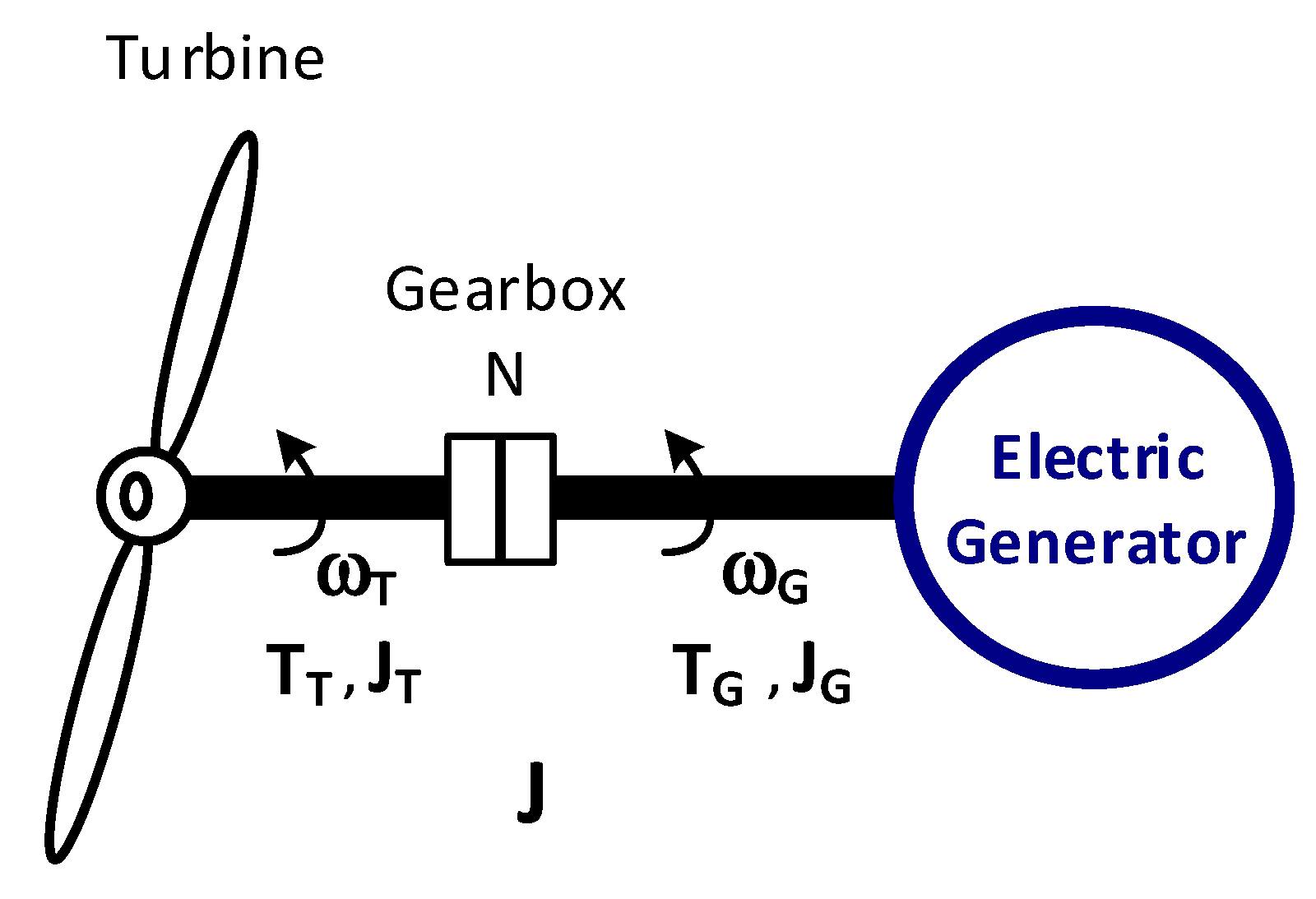
Figure 1 depicts a generic wind generator system. The wind turbine should have two or three blades and can be directly coupled to a permanent magnet synchronous generator (PMSG) or by means of a gearbox. The incoming aerodynamic turbine torque ($T_T$), produced by the action of the wind on the blades, is finally applied to the electrical generator, which in turn will generate a counter-electromagnetic torque ($T_G$). The moment of inertia ($J$) is the sum of the moments of inertia of both, the turbine ($J_T$), and the electrical generator ($J_G$):

$$J=J_T+J_G$$

(1)

Certain effects, like viscous friction coefficient and shaft torsional spring constant, are usually neglected to simplify the model. By means of this approximation, the mechanical model of the turbine can be expressed as follows:

$$\frac{T_T}{N}-T_G=J\frac{d{\omega }_G}{dt}$$

(2)

where ${\omega }_G$ is the angular speed of the electric PMSG generator and $N$ is the gear ratio of the gearbox. The power captured by a wind turbine depends on the interaction between the wind and the turbine blades. The power available in the wind ($P_{wind}$) is expressed as follows [5]:

$$P_{wind}=\frac{1}{2}\rho A{V}_{wind}^3$$

(3)

where $\rho$ is the density of the air (1225 kg/m³), $A$ is the area swept by the turbine blades given in m², and $V_{wind}$ is the wind speed given in $\mathrm{m}/\mathrm{s}$. The power coefficient $C_p$ is the ratio of the power captured by the wind turbine ($P_T$) on the low-speed shaft ($P_{LSS}$) to the power available in the wind, being expressed as follows:

$$C_p=\frac{P_{LSS}}{P_{wind}}=\frac{P_T}{P_{wind}}$$

(4)

Thus, the expression of $P_T$ can be obtained by combining (3) and (4) as follows:

$$P_T=\frac{1}{2}{C}_p\rho A{V}_{wind}{}^3$$

(5)

The maximum $C_p$ achievable by a turbine under ideal conditions is 0.59 (Betz limit). The power coefficient $C_p$ is a function of two parameters: the tip–speed ratio ($\lambda )$ and the pitch angle ($\beta$) of the blades. The tip–speed ratio relates the blade tip speed with the wind speed, and is expressed as follows:

$$\lambda =\frac{V_T}{V_{wind}}=\frac{{\omega }_T·r_T}{V_{wind}}$$

(6)

where V_T is the linear speed at the tip of the turbine blades, ${\omega }_T$ is the angular speed of the rotor of the turbine in rad/s, and $r_T$ is the length of the blade in m. The aerodynamic characteristic of a wind turbine can be modified by varying the pitch angle ($\beta$) of the blades. Such a technique, denoted as pitch control, is usually applied in large wind turbines, but is uncommon in small wind turbines.

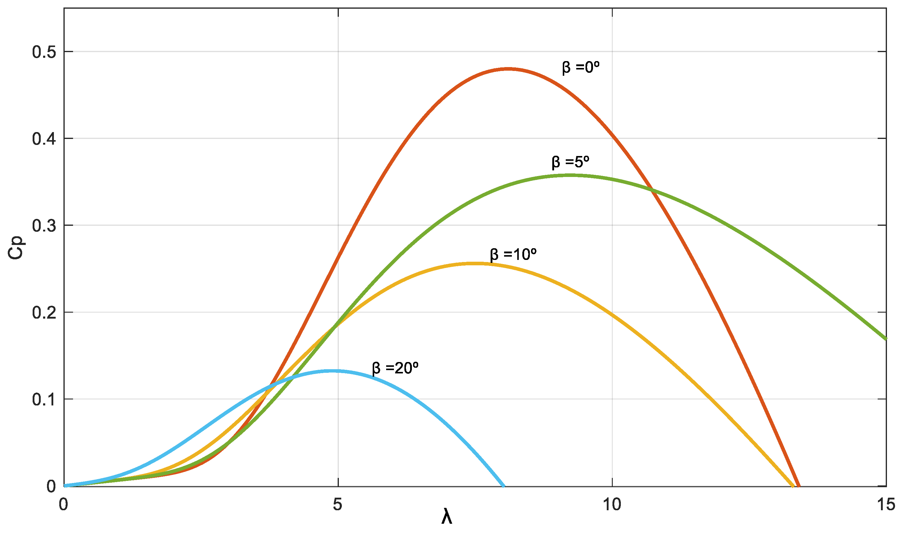
Figure 2 shows a set of $\lambda$-$C_p$ curves for different values of $\beta$, obtained using a non-lineal function [22]. Each curve has a different maximum power coefficient value, $C_{p_{max}}$, at a different $\lambda$ value (denoted as optimal lambda or ${\lambda }_{opt}$).

For small wind turbines, without pitch control, $\beta =0$. From Equation (5), the aerodynamic torque developed by a small wind turbine can be expressed as follows:

$$T_T=\frac{1}{2{\omega }_T}{C}_p\rho \mathrm{A}{V}_{wind}{}^3$$

(7)

The operating point of the wind turbine depends on the electrical power consumed by the electrical loads, as detailed in Equation (2).

3. Experimental Method for the Estimation of the $\mathit{\lambda }$-${\mathit{C}}_{\mathit{p}}$ Characteristic Curve of a Small Wind Turbine

Due to the high cost of the necessary tests, manufacturers do not offer the $\lambda$-$C_p$ characteristic curve of their small wind turbines. A knowledge of $\lambda$-$C_p$ characteristics is crucial for developing an efficient control of the energy conversion process, and securing the safe operation of the wind turbine. This section presents an experimental method developed for the estimation of the $\lambda$-$C_p$ characteristic curve of a small wind turbine without pitch control ($\beta =0$). This method is intended to give manufacturers of small wind turbines a practical and cheap tool to obtain the $\lambda$-$C_p$ characteristic curve of their turbines.

Given the difficulties of measuring $P_T$ in a commercial system and the low losses in the conversion from mechanical to electrical power when compared with the output electrical power, the value of C_p is usually calculated using the electrical generated power ($P_e$) [23]:

$$C_p=\frac{P_T}{P_{wind}}\cong \frac{P_e}{P_{wind}}$$

(8)

The $\lambda$-$C_p$ characteristic curve will be obtained after processing the data logged from several small wind turbines operating under real outdoor conditions. All of them are equipped with a specific firmware control that performs the test conditions required to acquire the following magnitudes: wind speed ($V_{wind}$); turbine angular speed (${\omega }_T$); and electrical generated power ($P_e$).

The small wind turbine used in the experimental parts of the paper is a Bornay Wind Plus 25.3+. This turbine is equipped with a set of three blades of $r_T$ = 2 m and has a moment of inertia $J$ = 5.75 Kg·m². The value of $\mathit{J}$ has been provided by the manufacturer and is the moment of inertia to be emulated. The turbine starts its operation for $V_{wind}$ > 3 m/s, develops the rated power for $V_{wind}$ = 12 m/s, and includes an automatic brake system if $V_{wind}$ > 14 m/s. The wind turbine is directly coupled to the shaft of the electrical generator, so N = 1. The electrical generator used in the Bornay Wind Plus 25.3+ is a permanent magnet synchronous generator (PMSG) and has the rated values shown in

Table 1. Technical characteristics of the electrical generator used in the small wind turbine.

Voltage	Rated Power (kW)	Peak Power (kW)	Rated Speed (rpm)	Pole Pairs
3–220 VL-L	5 kW	7 kW	375	8

.

Data is collected from three different small wind turbines, as part of three different off-grid systems. The presented results correspond to a two-month period of data recording. For data collection purposes, the control system of the turbine is modified to perform a speed reference (${\omega }_T^{*}$) sweep in a loop, varying from ${\omega }_{T_{min}}^{*}=$ 90 rpm to ${\omega }_{T_{max}}^{*}=$ 562.5 rpm (${1.5\mathsf{\omega }}_{T\_rated})$ with a 10 rpm increment every 30 min. Meanwhile, the system is sampling, every second, the three magnitudes needed to obtain the $\lambda$-$C_p$ points ($V_{wind}$, $P_e$, and ${\omega }_T$). To maintain ${\omega }_T$ constant, the electronic converter connected in the AC output of the PMSG must be able to extract all the generated electrical power. A controlled resistive load is used to extract the excess of power that the loads are not demanding. The data collection algorithm considers safety issues, resetting the speed reference to ${\omega }_{T_{min}}^{*}$ if the incoming torque exceeds a generator torque threshold that is set to 90% of the rated torque during the data recording. This limitation ensures that the maximum electrical torque of the generator is not exceeded, and the system can still be controlled. For every ${\omega }_T^{*}$ value, the system collects a huge amount of data that has to be filtered to discard non-significant values. 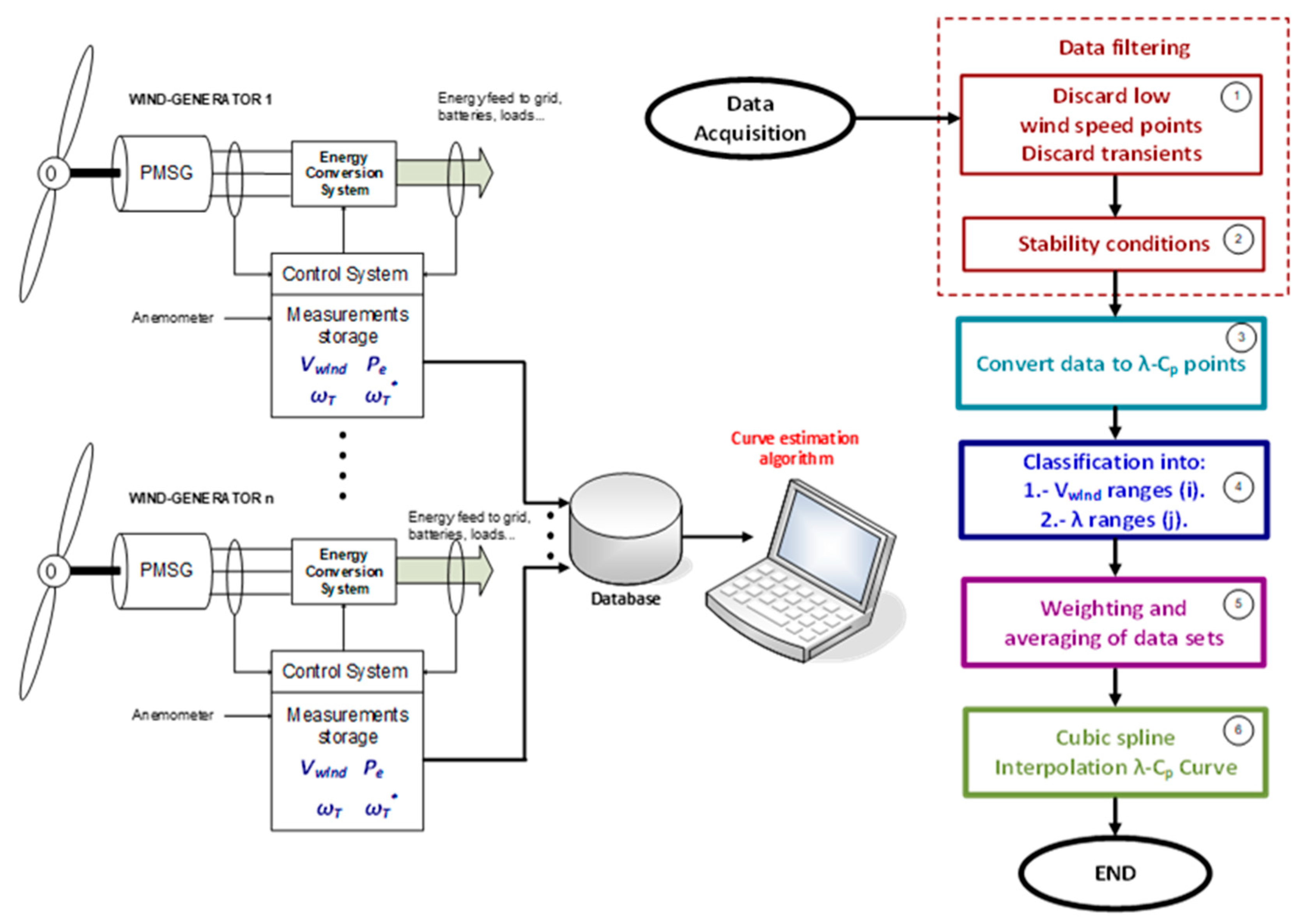Figure 3 depicts the block diagram of the acquisition system and the flowchart of the proposed algorithm for the estimation of the $\lambda$-$C_p$ characteristic curve.

A filtering process is started after the data recording. Since the wind turbines have a cut-in speed, all data collected corresponding to $V_{wind}$ < 3 m/s is discarded. The following filtering process is to delete the data corresponding to the transients, e.g., during wind speed changes. A set of values of $V_{wind}$, $P_e$, and ${\omega }_T$ is considered valid if the turbine angular speed is equal to its reference (${\omega }_T={\omega }_T^{*}$) and if $V_{wind}$ and ${\omega }_T$ are stable. The stability of $V_{wind}$ and ${\omega }_T$ is important because the turbine can store kinetic energy during transients. $V_{wind}$ and ${\omega }_T$ stability are verified by comparing the acquired sample (k) with the k − 4 and k + 4 samples (previous and subsequent recorded values, respectively). Maximum variation in $V_{wind}$ during the comparison is limited to ±1 m/s, while ${\omega }_T$ variation must be smaller than ±5 rpm.

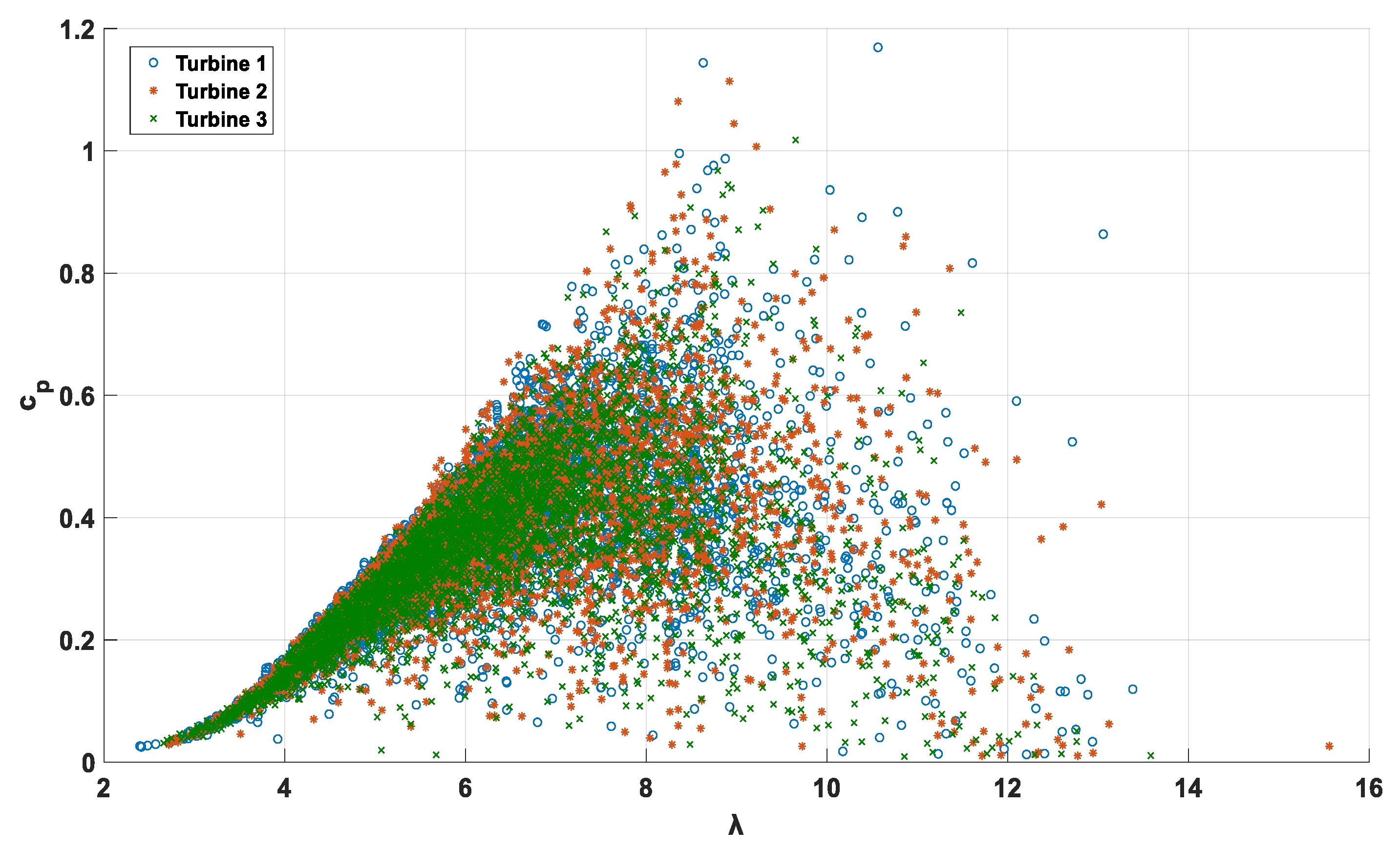
After the filtering process, the remaining sets of values of $V_{wind}$, $P_e$, and ${\omega }_T$ are processed to obtain the corresponding $\lambda$-$C_p$ coordinates. It is important to notice that the altitude has been considered to correct for air density when $C_p$ values are calculated. Figure 4 shows the $\lambda$-$C_p$ coordinates obtained after the filtering process. The points corresponding to each turbine are shown with different colors and symbols.

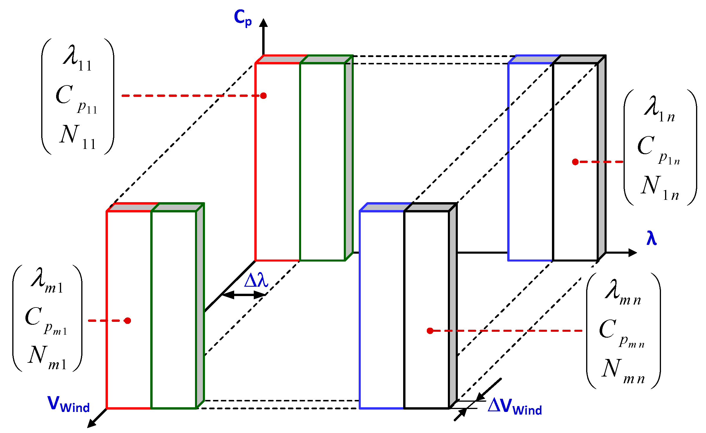
The obtained $\lambda$-$C_p$ points are classified firstly in $V_{wind}$ ranges, being denoted by subscript m in Figure 5. These ranges are selected in this study with $\Delta V_{wind}$ = 0.5 m/s, with acceptable values between 3 m/s (the cut-in speed of the turbine) to 16 m/s (m = 1…26). The points corresponding to each $V_{wind}$ range are classified again, this time in ranges of $\lambda$, being denoted by subscript n in Figure 5. These $\lambda$ ranges are selected to give enough resolution to the curve, Δ$\lambda$ = 0.1 being used in the experimental analysis, with a ${\lambda }_{max}=16$ for the turbines and locations used in the study. The three-dimensional space defined by $\lambda$-$C_p$-$V_{wind}$ is divided in m by n cuboids, as appears in Figure 5. A cuboid that contains less than five points is discarded because they are non-representative points of the $\lambda$-$C_p$ curve.

The total number of $\lambda$-$C_p$-$V_{wind}$ points in each cuboid is an element N_ij of matrix N, where i = 1‥m and j = 1‥n, expressed as follows:

$$\mathbf{N}=\left(\begin{array}{ccc}{N}_{11}& \cdots & N_{1n}\\ ⋮& \ddots & ⋮\\ N_{m1}& \cdots & N_{mn}\end{array}\right)$$

(9)

The points inside each cuboid are averaged to obtain one unique point per cuboid, obtaining the following matrix of $\lambda$-$C_p$ coordinates:

$$\mathsf{\lambda }\text{-}{\mathbf{C}}_{\mathbf{p}}=\left(\begin{array}{ccc}{\left(\lambda -C_p\right)}_{11}& \cdots & {\left(\lambda -C_p\right)}_{1n}\\ ⋮& \ddots & ⋮\\ {\left(\lambda -C_p\right)}_{m1}& \cdots & {\left(\lambda -C_p\right)}_{mn}\end{array}\right)$$

(10)

To obtain only one $\lambda$-$C_p$ point for each ${\lambda }_j$ range, a weighted average process is applied considering the m different points contained inside each range. The weighting factor relates the number of samples averaged inside each cuboid to the total number of samples inside each ${\lambda }_j$ range, thus the more points inside a cuboid the greater the contribution of that cuboid to the resulting $\lambda$-$C_p$ coordinate. The weighting factor $w_{ij}$ applied to each $(\lambda$-$C_p{)}_{ij}$ point is calculated as in Equation (11).

$$w_{ij}=\frac{N_{ij}}{N_j}$$

(11)

where $N_j$ is the total number of points in each ${\lambda }_j$ range. $\mathbf{W}$ is the weights matrix, defined as follows:

$$\mathbf{W}=\left(\begin{array}{ccc}{w}_{11}& \cdots & w_{1n}\\ ⋮& \ddots & ⋮\\ w_{m1}& \cdots & w_{mn}\end{array}\right)$$

(12)

The B row vector that contains the $\lambda$-$C_p$ points that describe the characteristic curve of the turbines is calculated as follows:

$$\mathbf{B}=W^T\times \left(\mathsf{\lambda }-{\mathbf{C}}_{\mathbf{p}}\right)$$

(13)

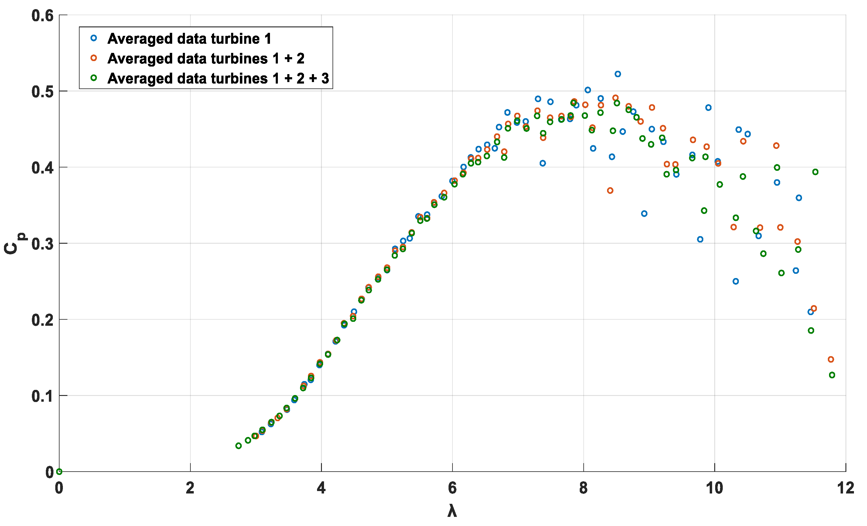
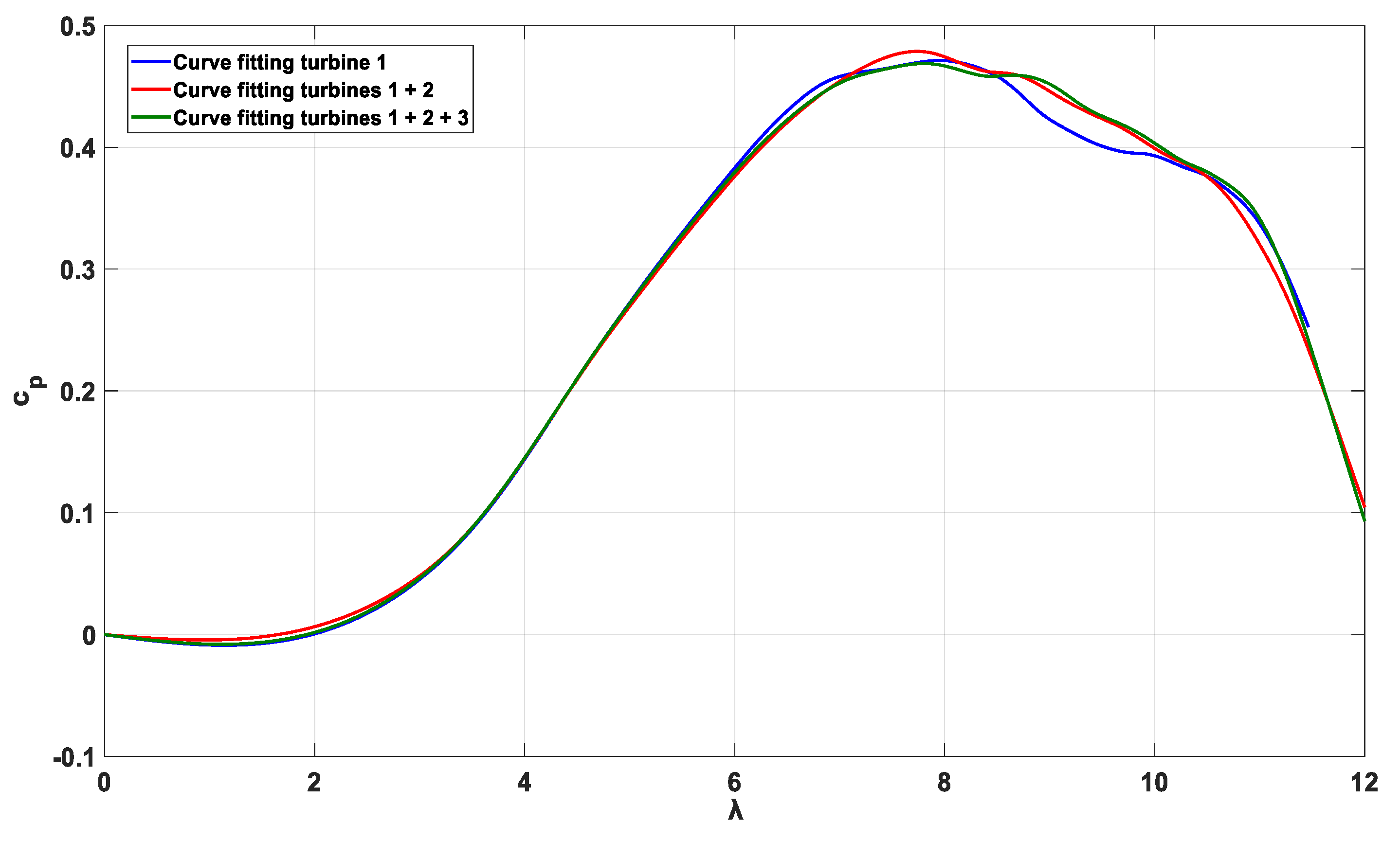
Figure 6 shows the averaged and weighted points obtained for three aggregation cases: using the data from turbine 1 (blue), merging the data from turbines 1 and 2 (red), and using the combined data from the three turbines (green).

The resulting $\lambda$-$C_p$ points should be then interpolated (step 6 in Figure 3) to obtain the characteristic $\lambda$-$C_p$ curve of the turbine. For this purpose, an interpolation method must be selected. To assess the fitting of the estimated curve, the parametric continuity condition is used. In general, a higher order of parametric continuity means a smoother curve with softer gradients. A curve can be said to have ${\mathit{C}}^{\mathit{n}}$ parametric continuity when its $n$th derivative $\left(\frac{d^{n}y}{d{x}^n}\right)$ is continuous throughout the curve. Linear interpolation will yield a curve with relatively poor smoothness, usually presenting abrupt gradient changes. The resulting curve of a linear interpolation will have zero-order parametric continuity (denoted as ${\mathit{C}}^{\mathbf{0}}$). Polynomial interpolation methods may result in curves with second-order (or higher) parametric continuity, but this method may also suffer from Runge’s phenomenon, which appears when applying high-order polynomials to evenly spaced data sets. The cubic spline interpolation method constructs a curve in a piecewise-polynomial fashion. The resulting curve is generated piece-by-piece by applying a low-degree polynomial function for every piece, presenting ${\mathit{C}}^{\mathbf{0}}$, ${\mathit{C}}^{\mathbf{1}}$ and ${\mathit{C}}^{\mathbf{2}}$ parametric continuity. Cubic spline interpolation has a smaller error than linear interpolation and the resulting interpolant function (the $\lambda$-$C_p$ curve of the turbine) is easier to evaluate than when polynomial interpolation is used. Due to these characteristics, cubic spline interpolation has been selected as the interpolation method.

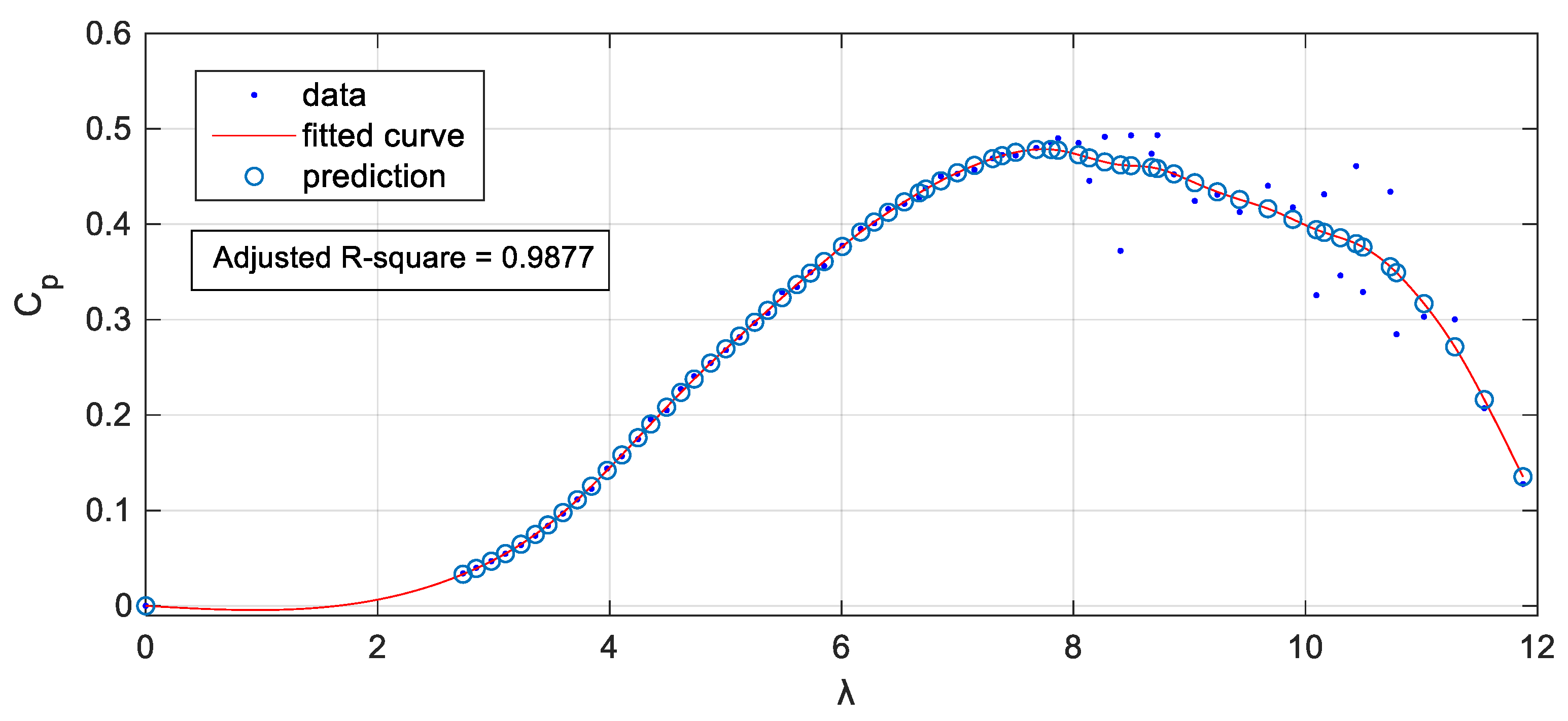
The resulting $\lambda$-$C_p$ points obtained for this set of turbines are shown as blue dots in Figure 7. It can be seen that the maximum $C_p$ never exceeds 0.5, which is always below the Betz limit. Distribution of points until reaching ${\lambda }_{opt}$ is quite uniform, with a greater dispersion for $\lambda >{\lambda }_{opt}$.

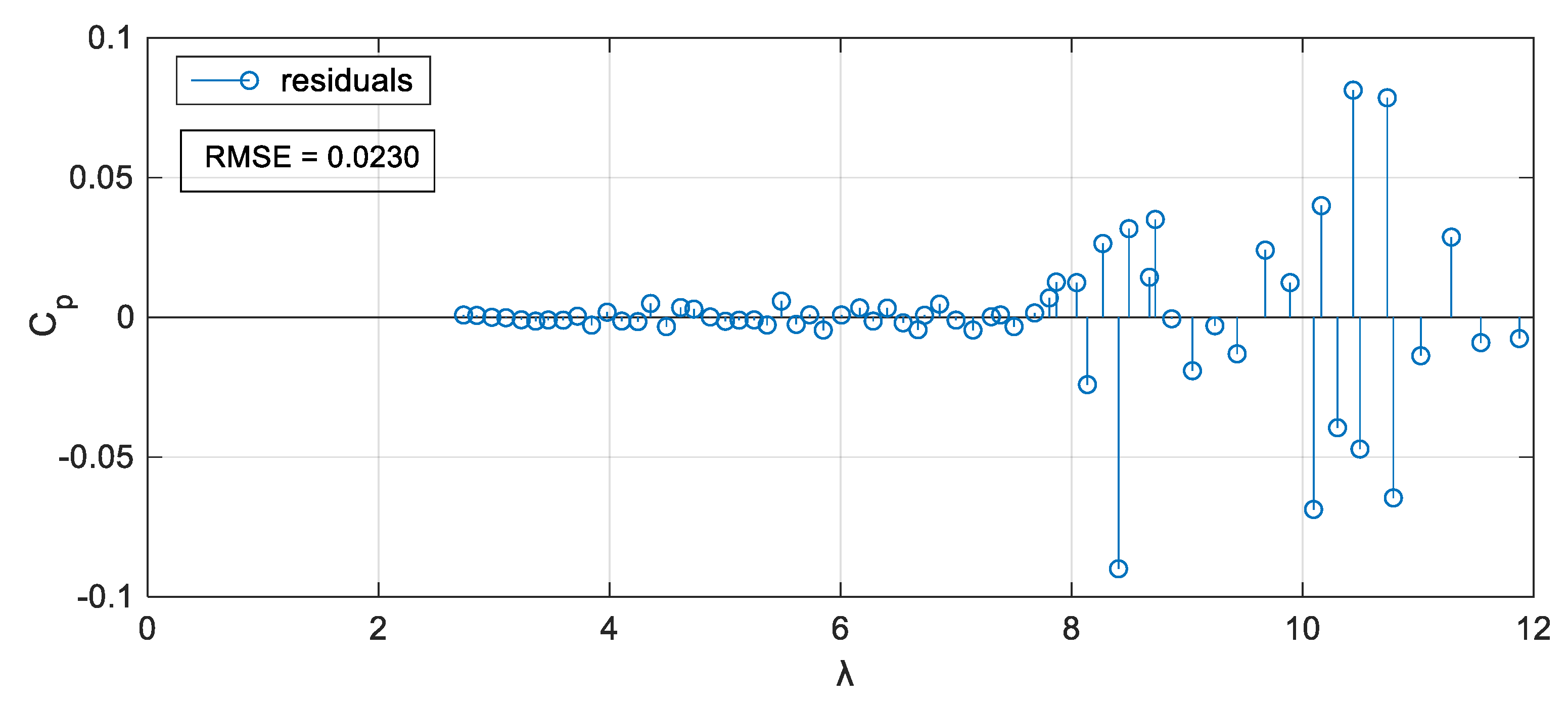
The red curve in Figure 7 is the result obtained after applying the cubic spline interpolation. Figure 7 shows the interpolated points that define the fitting curve along with the averaged points. This figure shows how the spline function, while not being able to pass through every data point, bends the curve to fit the overall trend of the data set. Figure 8 shows the residuals between the interpolated curve and the points used for interpolation. To validate the goodness of fit, some statistical factors have been calculated. The adjusted R-square parameter measures how successful the fit is in explaining the variation of the data. In this case, adjusted R-square of 98.77% implies a very good fit. The root mean square of error is equal to 0.023.

The $\lambda$-$C_p$ curve estimation improves as more data is fed to the proposed algorithm. Figure 9 shows how the interpolated curve varies as new data is aggregated, showing the curves obtained for the three cases.

Analyzing the averaged series, it can be seen that there is no data for $\lambda$ values below 2.3, so the actual estimated curve starts around $\lambda =2$. The low-side of the $\lambda$-$C_p$ curve (values below $\lambda =2$) is interpolated from zero to the first available point, keeping the first and second derivatives of the joined curves equal. Although the default value of the first point is $\left(0,0\right)$, it is important to notice that it should be defined by the starting torque of the wind turbine. 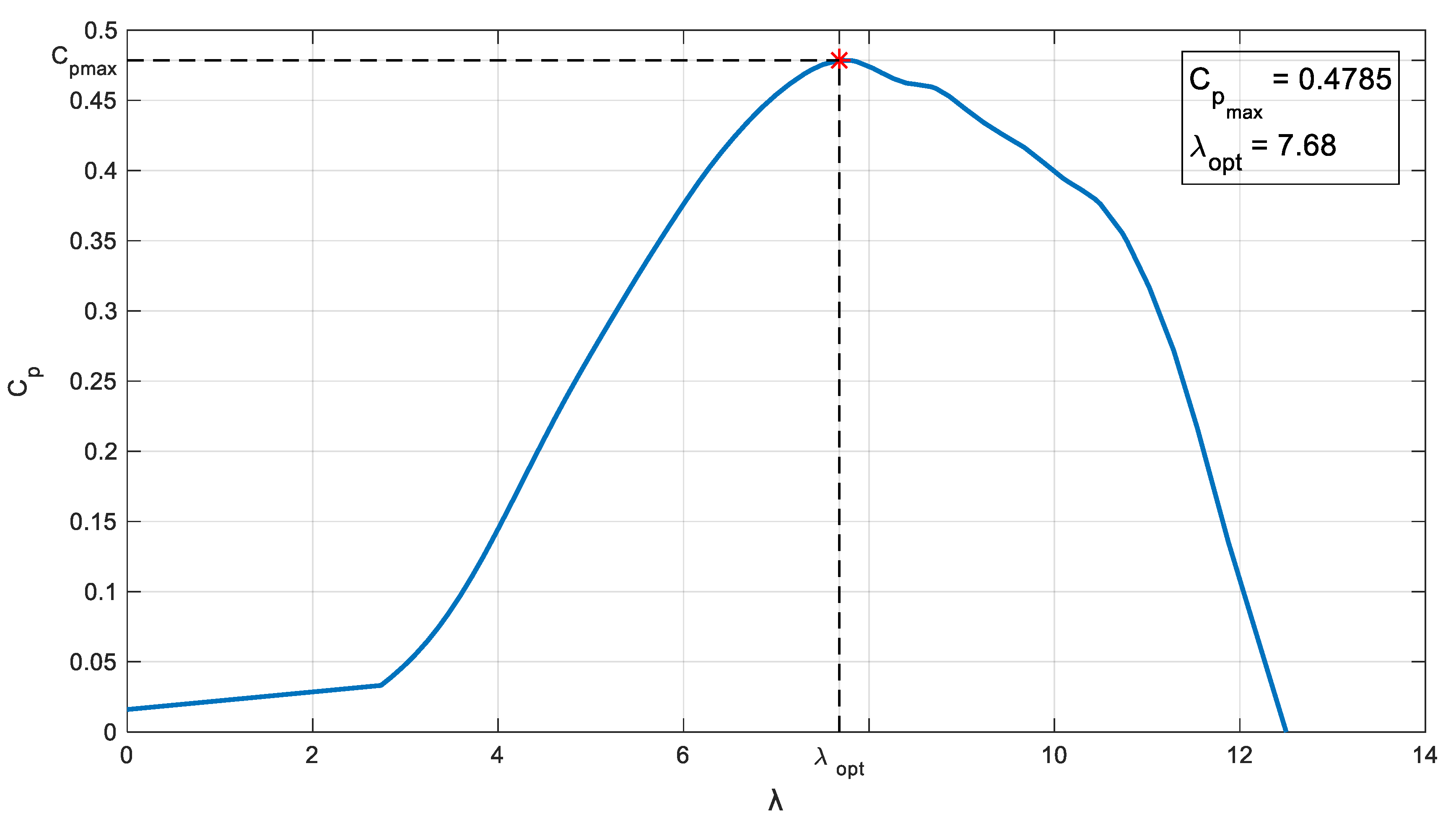In Figure 10, the final $\lambda$-$C_p$ curve of the turbines is shown.

The curve reaches a maximum $C_p$ value of 0.4785 at $\lambda$ = 7.68. This point represents the maximum efficiency achievable for the system. The resulting curve also considers the starting torque of the real model.

4. Proposed Small Wind Turbine Emulator

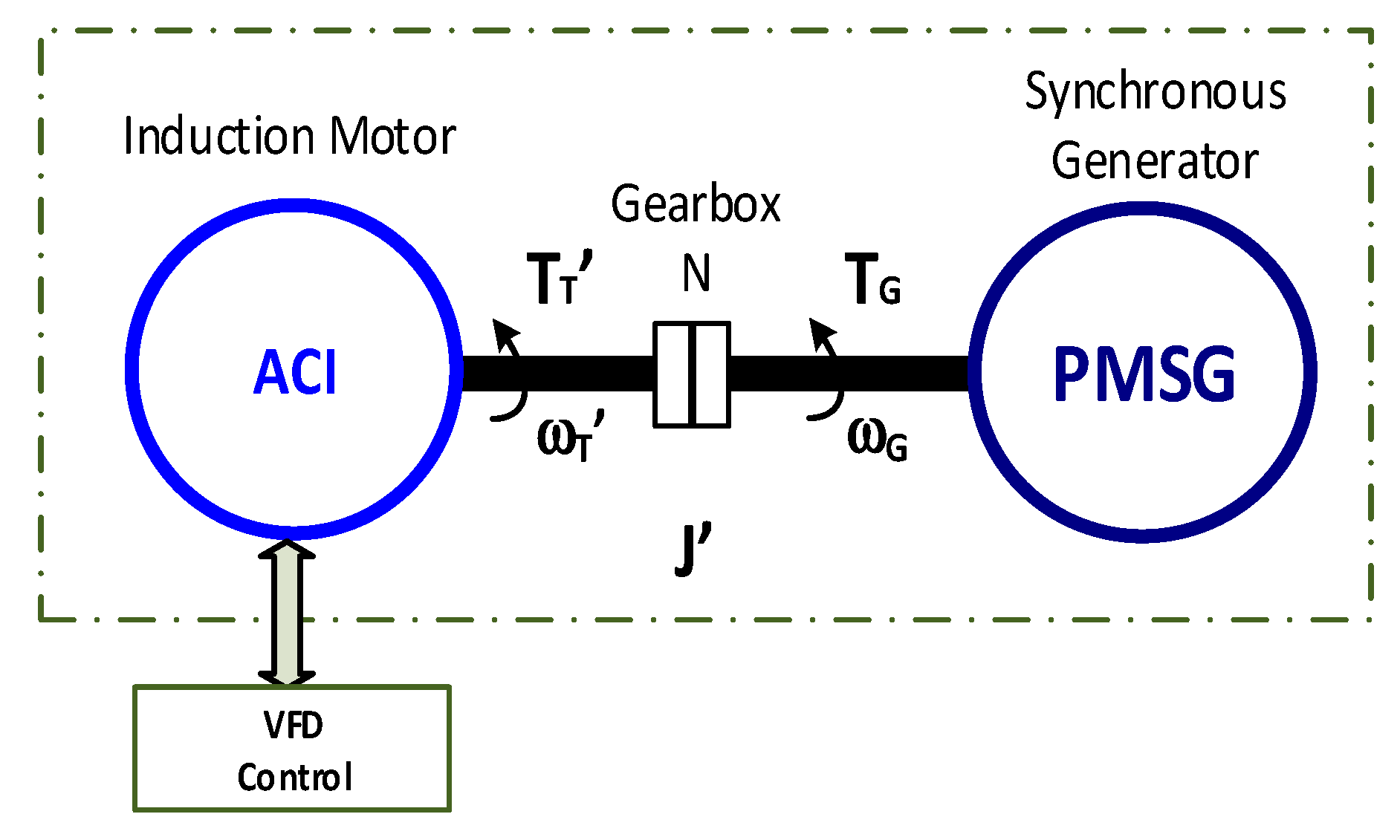
The mechanical model of the proposed emulator is shown in Figure 11, where $T_T{}^{\prime }$ is the torque delivered by the induction motor that is emulating the turbine operation, $N$ is the gear ratio of the gearbox, and $J^{\prime }$ is the moment of inertia of the mechanical system including the induction motor (IM block), the gearbox, and the PMSG generator. The emulator is implemented with the same PMSG generator used in the wind turbines used to obtain the $\lambda$-$C_p$ curve.

From Figure 11, the rotational dynamics of the proposed wind turbine emulator are expressed as follows:

$$\frac{T_T{}^{\prime }}{N}-T_G=J^{\prime }\frac{d{\omega }_G}{dt}$$

(14)

It should be noted that $J^{\prime }$ must be smaller than $J$ in order to achieve the same dynamic response as the real turbine, compensating the moment of inertia in a similar way to that described in References [17,18]. Basically, emulation of a moment of inertia greater than $J^{\prime }$ can be achieved by controlling the speed reference variation of the induction motor controller during accelerations or decelerations.

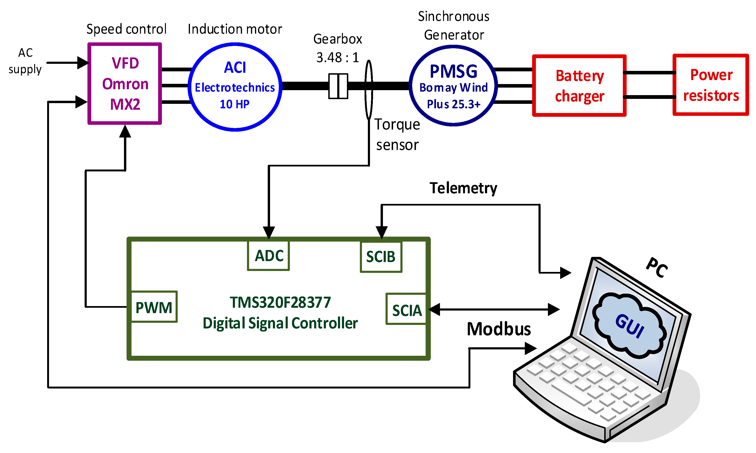
A detailed block diagram of the proposed emulator is shown in Figure 12. A control algorithm that implements Equation (7) determines the control signal applied to the variable-frequency drive (VFD) that, along with the induction motor, simulates the wind turbine. The gearbox enables the induction motor to apply a higher torque to the electric generator side. Therefore, the rated torque of the induction motor might be smaller than the rated torque of the electric generator ($T_T{}^{\prime }<T_G$) and still be able to emulate the operating point of the turbine on either side of the power curve for testing purposes.

The emulated wind torque is provided by an induction motor produced by Electrotechnics (230/400 V/50 Hz, 10 HP, 1460 rpm, $\cos \varphi =0.85$), controlled by an Omron 3G3MX2-A4110-E variable-frequency drive, with the rated characteristics shown in

Table 2. Technical characteristics of the variable-frequency drive used in the emulator.

Voltage Class	Constant Torque Control Mode		Variable Torque Control Mode
	Max Power (kW)	Rated Current (A)	Max Power (kW)	Rated Current (A)
3–400 VL-L	11	24	15	31

.

The VFD drive implements a sensorless speed control. The speed reference of the VFD drive is proportional to the frequency of a pulse train applied to an input equipped with a capture module. The induction motor and the PMSG are linked by a gearbox with a gear ratio $N=3.48:1$. The PMSG is part of the Bornay Wind Plus 25.3+ small wind turbine and its main characteristics have been described in a previous section. The energy generated by the PMSG must be dissipated by an intelligent load that can be controlled to set different loading situations.

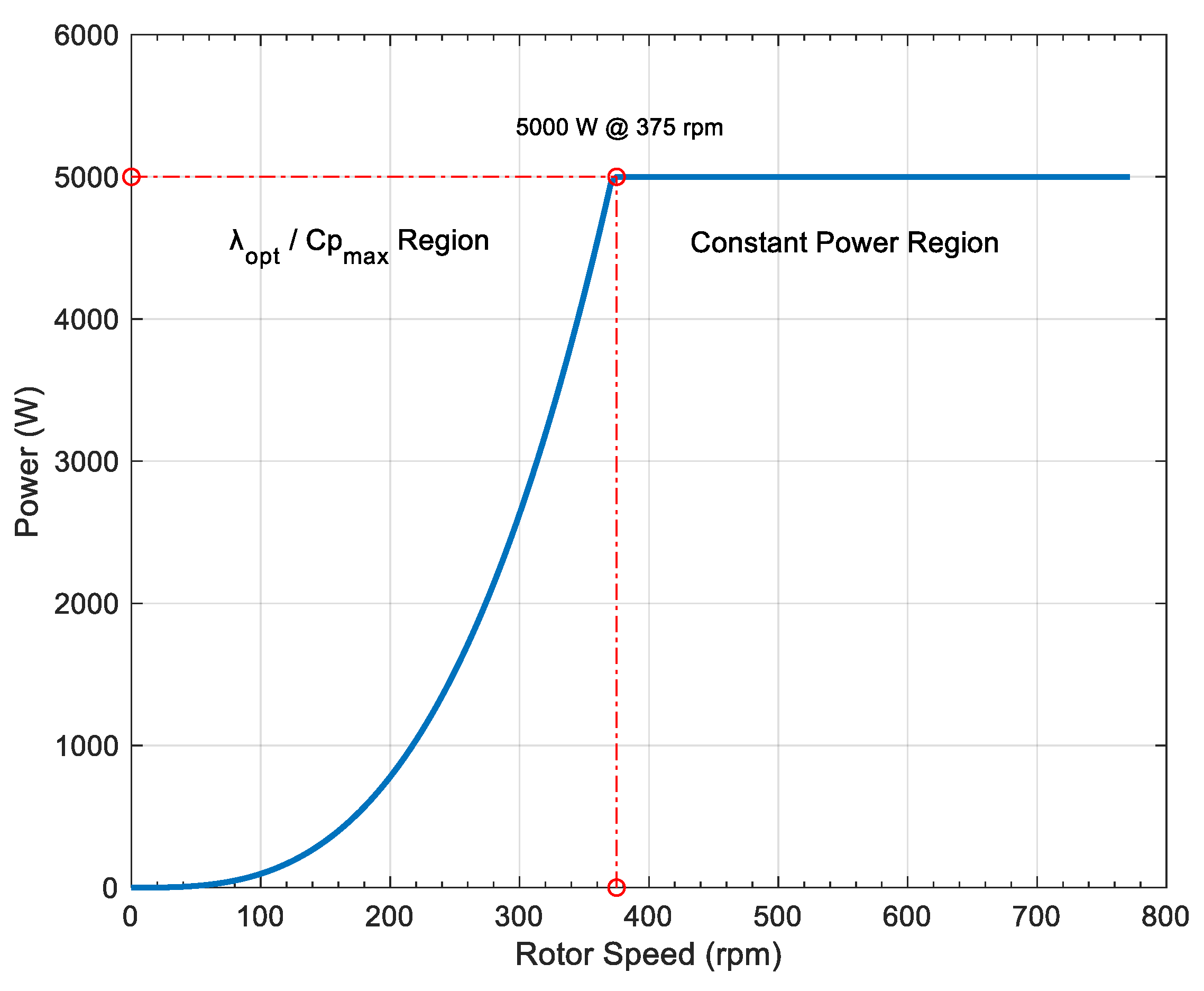
In the proposed emulator, a battery charger and some power resistors implement this intelligent load. The battery charger used in the emulator is part of the solution provided by the manufacturer when the Bornay Wind Plus 25.3+ small wind turbine is used in off-grid systems. Figure 13 details the power vs speed curve used to establish the battery charging current. In this way, for a given rotational speed the battery charger will generate the necessary load torque. The battery charger is equipped with resistors that dissipate the surplus energy and maintain the battery voltage in the floating range, and so avoiding overcharging the battery.

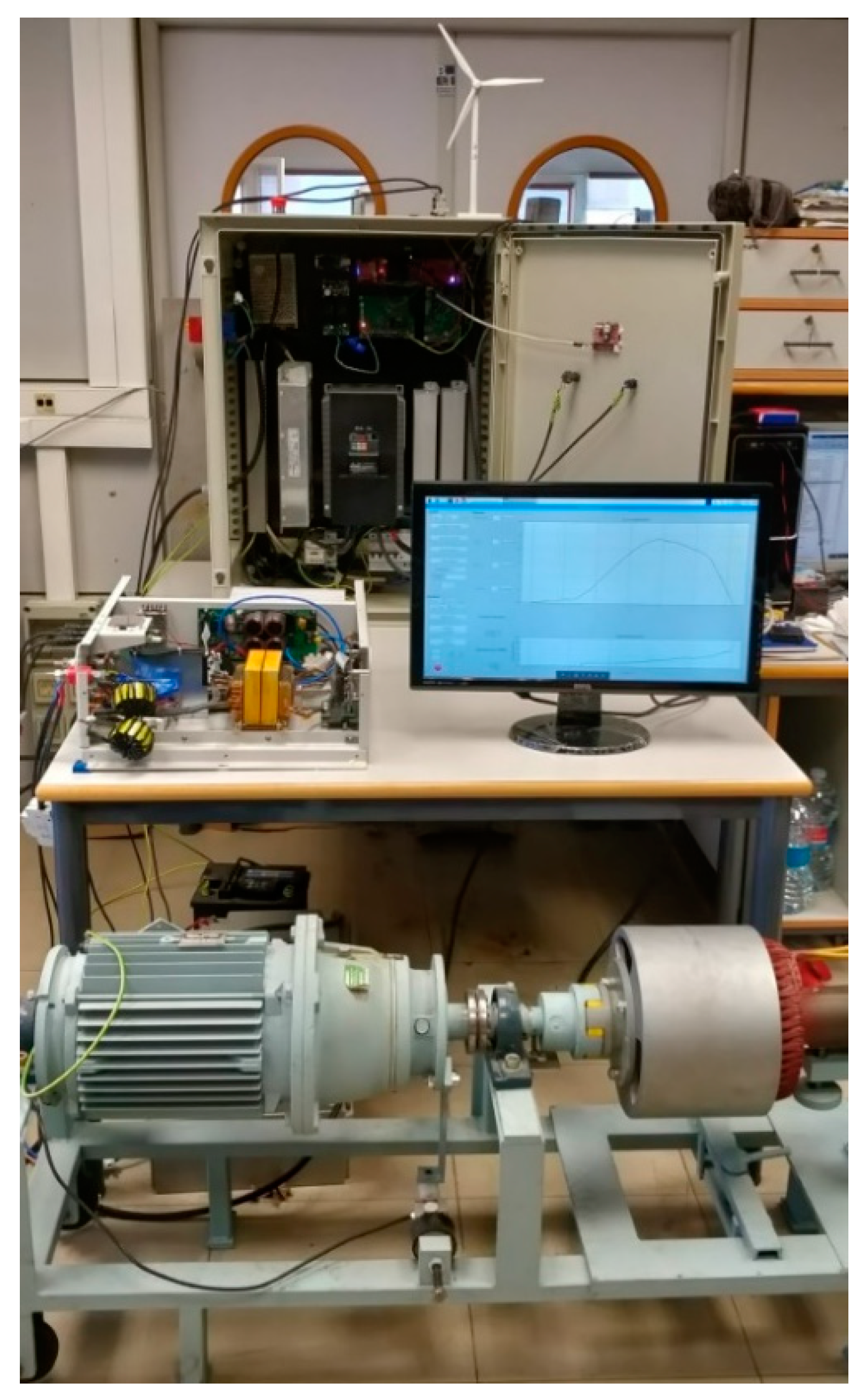
Figure 14 shows the parts of the small wind turbine emulator system: the motor-generator bench in front, followed by the display that shows the GUI (right) and the battery charger (left), and behind is the electric box that contains the VFD drive that controls the induction motors that simulate the turbine (left, front). A gear box connects both shafts.

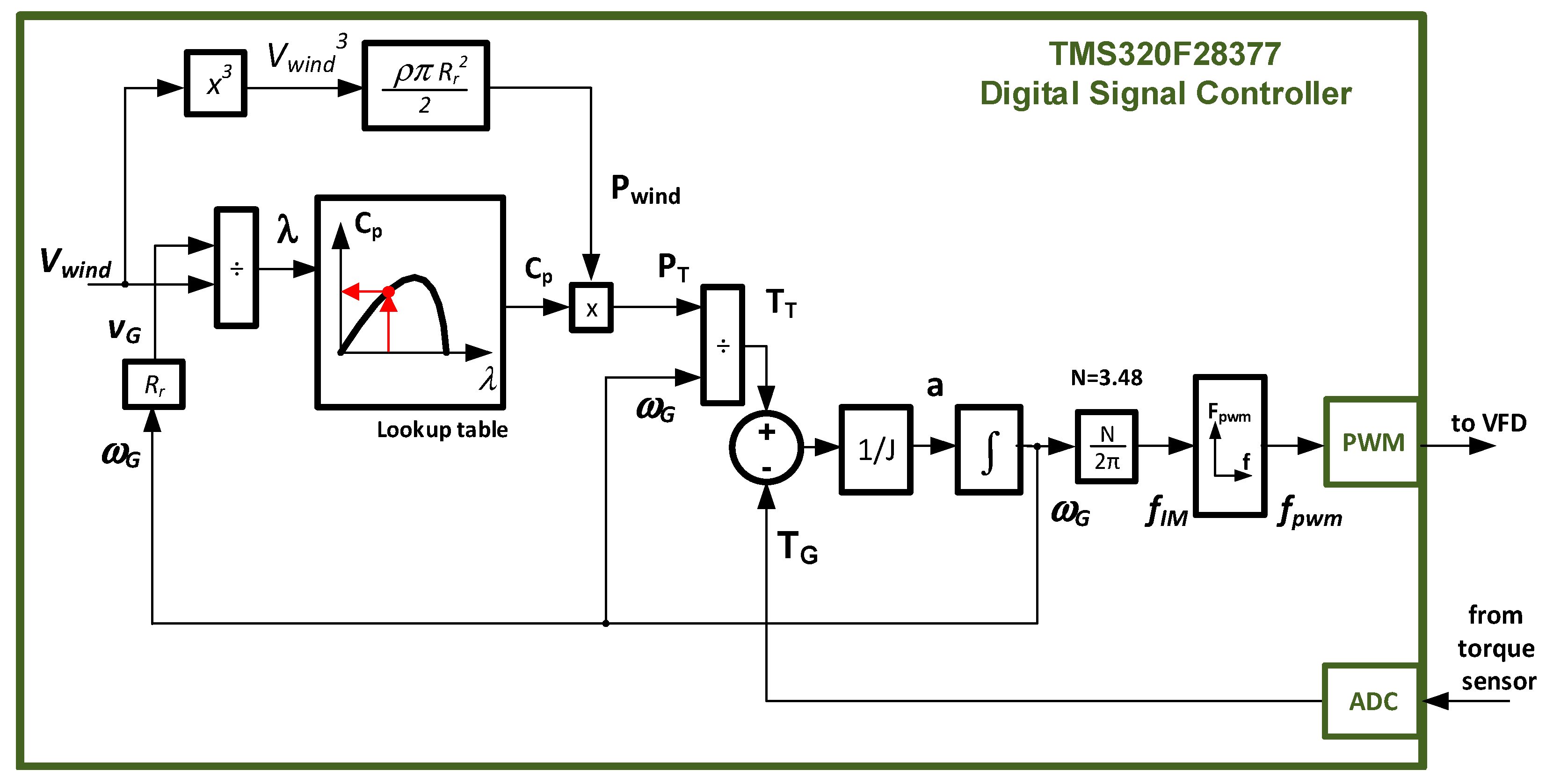
The main control of the turbine emulator system is made by a Texas Instruments TMS320F28377 digital signal controller (DSC). Based on the mechanical model, the inertia to be simulated, and the $\lambda$-$C_p$ curve obtained in the previous section, the DSC determines the speed reference of the induction motor. The block diagram of the algorithm implemented in the DSC is depicted in Figure 15. The block diagram implemented corresponds to a directly coupled small wind turbine, so Equation (2) is used and the gear ratio N is added after ${\omega }_G$ is calculated.

The emulated wind speed is applied to Equation (3) to determine the available wind power (P_wind). Wind and turbine speeds are replaced in Equation (6) to obtain the corresponding $\lambda$ value. At this point, a lookup table with the $\lambda$-$C_p$ curve has to be accessed to obtain the actual $C_p$ value. The $\lambda$-$C_p$ curve is stored in the memory of the DSC as a table. From these results and by applying Equation (5), the power captured by the turbine (P_T) is computed. The incoming aerodynamic torque ($T_T$) is obtained by dividing the captured power by the directly coupled turbine speed (${\omega }_T={\omega }_G$). By calculating the torque difference and using the value of the moment of inertia J to be emulated, the system acceleration (“a” in Figure 15) can then be found from Equation (2). Finally, considering the gearbox ratio, the turbine speed reference signal to feed the speed control input of the VFD drive is obtained by integrating the resulting acceleration.

To validate the proposed small wind turbine emulator system, the experimental $\lambda$-$C_p$ curve of Figure 10 has been programmed into the emulator and two experiments have been carried: first, to validate the implementation of the mechanical model, a series of $J$ variations are made; in the second experiment, the emulator is tested along with the GUI.

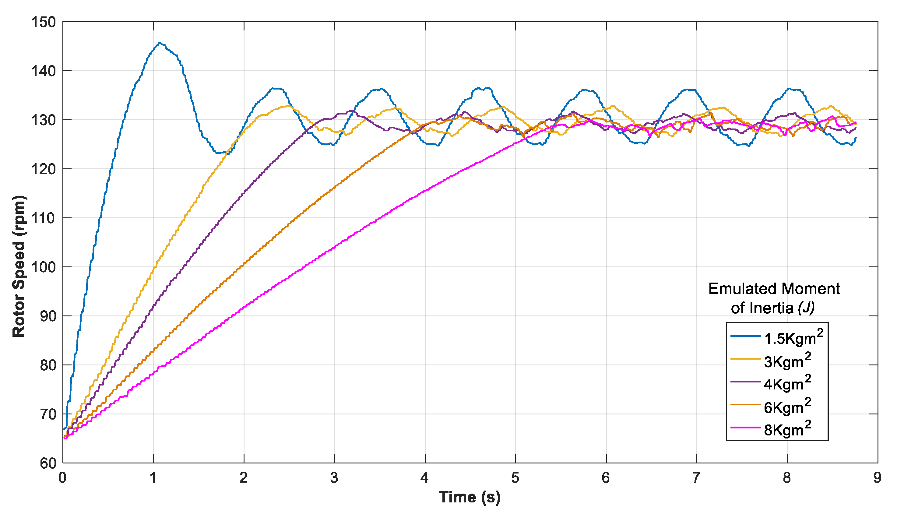
For the first test, the wind speed is set to a fixed value, battery charger is configured to control the angular speed of the turbine at a set point of 130 rpm, and the speed controller in the battery charger is tuned to control the real turbine. By maintaining the turbine angular speed reference constant, it is verified that the dynamic response of the system varies with the emulated moment of inertia ($J$), as can be seen for the different cases shown in Figure 16. As $J$ increases, the system response becomes slower, as if the system was getting heavier. This demonstrates that the proposed emulator could emulate the dynamic response of any wind turbine that meets the condition that the moment of inertia of the system to be emulated is greater than the moment of inertia of the emulator.

$$J>J^{\prime }$$

Figure 16 also shows how the response of the speed regulator oscillates accordingly to the value of the moment of inertia. This is because the control of the intelligent load is tuned to work with the Wind Plus 25.3+ turbine ($J$ = 5.75 Kg·m²), as was explained previously. This means that the same controller has a different response when the value of $J$ is changed; that is, the load sees a different turbine.

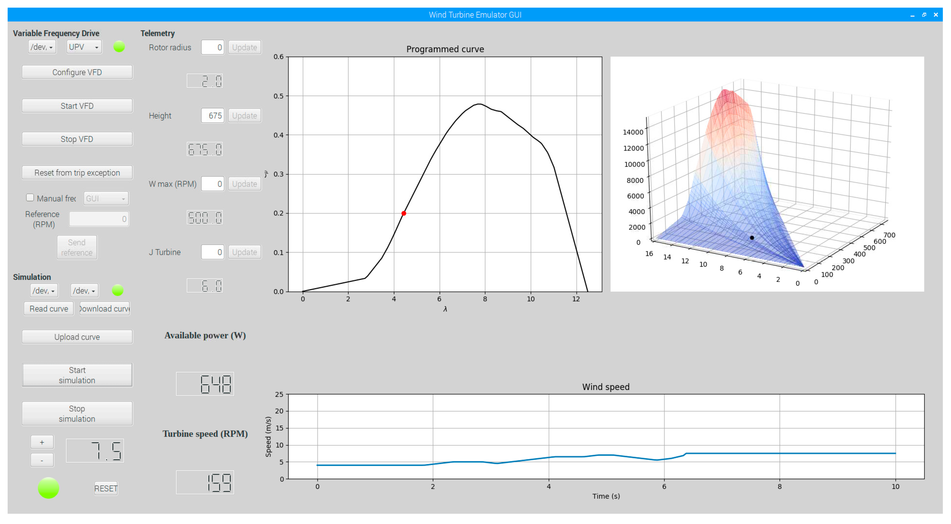
The graphic user interface developed to manage the small wind turbine emulator is shown in Figure 17. Through the GUI, it is possible to configure the VFD drive and communicate with the DSC to start/stop the emulation. In addition, the following emulation parameters can be set inside the GUI environment: rotor radius; height above sea level; speed limit; moment of inertia of the system; wind speed; $\lambda$-$C_p$ characteristic curve of the turbine to emulate (left side of the GUI in Figure 17). The GUI also displays a real-time visualization of the operating point of the emulated turbine, both in the $\lambda$-$C_p$ curve and in the working surface of the turbine (right section in Figure 17); as well as the emulated wind speed (bottom section in Figure 17).

Figure 17 shows the surface of the turbine and the operating point. From the trajectory described by the operating point, the convergence of the models is validated, and the emulator operates at all times on the surface obtained from the experimental data collected. The $\lambda$-$C_p$ curve is also shown (upper graph in the center of the GUI screen) along with the real-time $C_P$ value (red dot over the $\lambda$-$C_p$ curve), confirming that the emulator presents the same behavior as the real turbine modeled.

The results shown above demonstrate the convergence between the implemented emulator and the model generated from the proposed analysis methodology that is based on the data obtained from three real wind turbines. The experimental $\lambda$-$C_p$ curve is uploaded in the GUI and then sent to the DSC that controls the motor/generator bench. The GUI builds and shows the working surface of the corresponding turbine. When the emulator is working, the GUI shows the trajectory of the operating point over the working surface of the turbine. The operation in a stable point located at ${\lambda }_{opt}$ demonstrates that the model implemented in the DSC is working correctly and corresponds to that obtained from the real data.

5. Conclusions

The implementation of a realistic small wind turbine emulator system has been addressed in this paper. It is based on the use of the electrical generator and the $\lambda$-$C_p$ characteristic curve of the real small wind turbine to be emulated. To validate the proposed emulator, a Bornay Wind Plus 25.3+ wind turbine has been used in this work.

An experimental method for the estimation of the $\lambda$-$C_p$ characteristic curve of small wind turbines is proposed. This method avoids the need for expensive wind tunnels; however, a working wind turbine is needed and, depending on the wind conditions, it could take some time to collect enough data to obtain the $\lambda$-$C_p$ characteristic curve. A cubic spline interpolation has been used to obtain a smooth $\lambda$-$C_p$ curve, which presents a C² parametric continuity.

Different aggregations of the data obtained with the three small wind turbines used in the experimental tests are compared. The obtained results demonstrate how the interpolated $\lambda$-$C_p$ curve improves when more data sets are used in the process.

A graphic user interface has been developed to configure and monitor the operation of the emulated small wind turbine. It also represents the working surface of the turbine and the real time turbine operating point during the simulation.

The experimental results demonstrate that the dynamic response of the system varies with the emulated moment of inertia, and that the proposed emulator could emulate the dynamic response of any wind turbine with a moment of inertia greater than the moment of inertia of the emulator. The emulator always operates on the working surface obtained from the experimental data collected, demonstrating the convergence between real and emulated systems, showing that the model agrees with that obtained experimentally, and that the emulator works properly.

The proposed emulator will improve the design process and validation of power electronic converters, control strategies, and characterization of the PMSG of small wind turbine systems, by using the real $\lambda$-$C_p$ characteristic curve of the wind turbine.