Optimal Sizing of Battery Energy Storage for a Grid-Connected Microgrid Subjected to Wind Uncertainties

Abstract

In this paper, based on stochastic optimization methods, a technique for optimal sizing of battery energy storage systems (BESSs) under wind uncertainties is provided. Due to considerably greater penetration of renewable energy sources, BESSs are becoming vital elements in microgrids. Integrating renewable energy sources in a power system together with a BESS enhances the efficiency of the power system by enhancing its accessibility and decreasing its operating and maintenance costs. Furthermore, the microgrid-connected BESS should be optimally sized to provide the required energy and minimize total investment and operation expenses. A constrained optimization problem is solved using an optimization technique to optimize a storage system. This problem of optimization may be deterministic or probabilistic. In case of optimizing the size of a BESS connected to a system containing renewable energy sources, solving a probabilistic optimization problem is more effective because it is not possible to accurately determine the forecast of their output power. In this paper, using the stochastic programming technique to discover the optimum size of a BESS to connect to a grid-connected microgrid comprising wind power generation, a probabilistic optimization problem is solved. A comparison is then produced to demonstrate that solving the problem using stochastic programming provides better outcomes and to demonstrate that the reliability of the microgrid improves after it is connected to a storage system. The simulation findings demonstrate the efficacy of the optimum sizing methodology proposed.

1. Introduction

The importance of green energy and renewable energy sources increases to save the environment. When it comes to renewable energy sources, it is very important to talk about energy storage systems (ESS) and their applications in microgrids integrated with renewable energy. ESSs also have the ability to enhance the microgrid reliability and lower costs. In order to connect an ESS to a microgrid, the optimal size must be found. Many methods and techniques have been developed to find the optimal size of an ESS.

This paper describes a method for optimally sizing an ESS to be incorporated into a microgrid linked to a main grid under wind uncertainties to improve the accuracy and reliability of the microgrid using the stochastic programming method. In the literature, some papers have been written about the optimal sizing of a storage system in a microgrid. However, sizing a storage system under generation uncertainties is missing. In reality, a new model has been suggested to optimize the size of an energy storage system taking into account wind uncertainties in system modeling, which is of critical importance in power systems with intermittent renewable energy sources such as wind. In addition, the proposed model is developed with an additional objective of enhancing system reliability particularly with the incorporation of reliability constraints. The reliability-constrained optimization problem under the influence of wind uncertainties is solved and a comparison between two cases has been made to appreciate the effects of the optimally sized storage system on the microgrid reliability and to investigate how the microgrid reliability enhances.

The rest of the paper is arranged as follows. The literature review in Section 2 summarizes latest field-related articles. Section 3 describes the equations used to calculate the optimum size of an ESS and indices of reliability. Section 4 presents a straightforward case study used to evaluate an ESS’ suggested optimum sizing method. Section 5 demonstrates and illustrates the outcomes of the simulation after resolving the case study optimization problem. Section 6 is the paper’s conclusion.

2. Literature Review

Microgrids are small-sized power systems. Microgrids are intended and constructed to provide electrical energy to clients linked to them. Microgrids could be isolated or connected to the grid [1]. The microgrid can exchange energy if it is attached to the main grid by importing and exporting it to the main grid. Microgrid characteristics include distributed generators, renewable energy sources, storage devices, and controllable loads [2]. These characteristics make microgrids more flexible, reliable and effective [3].

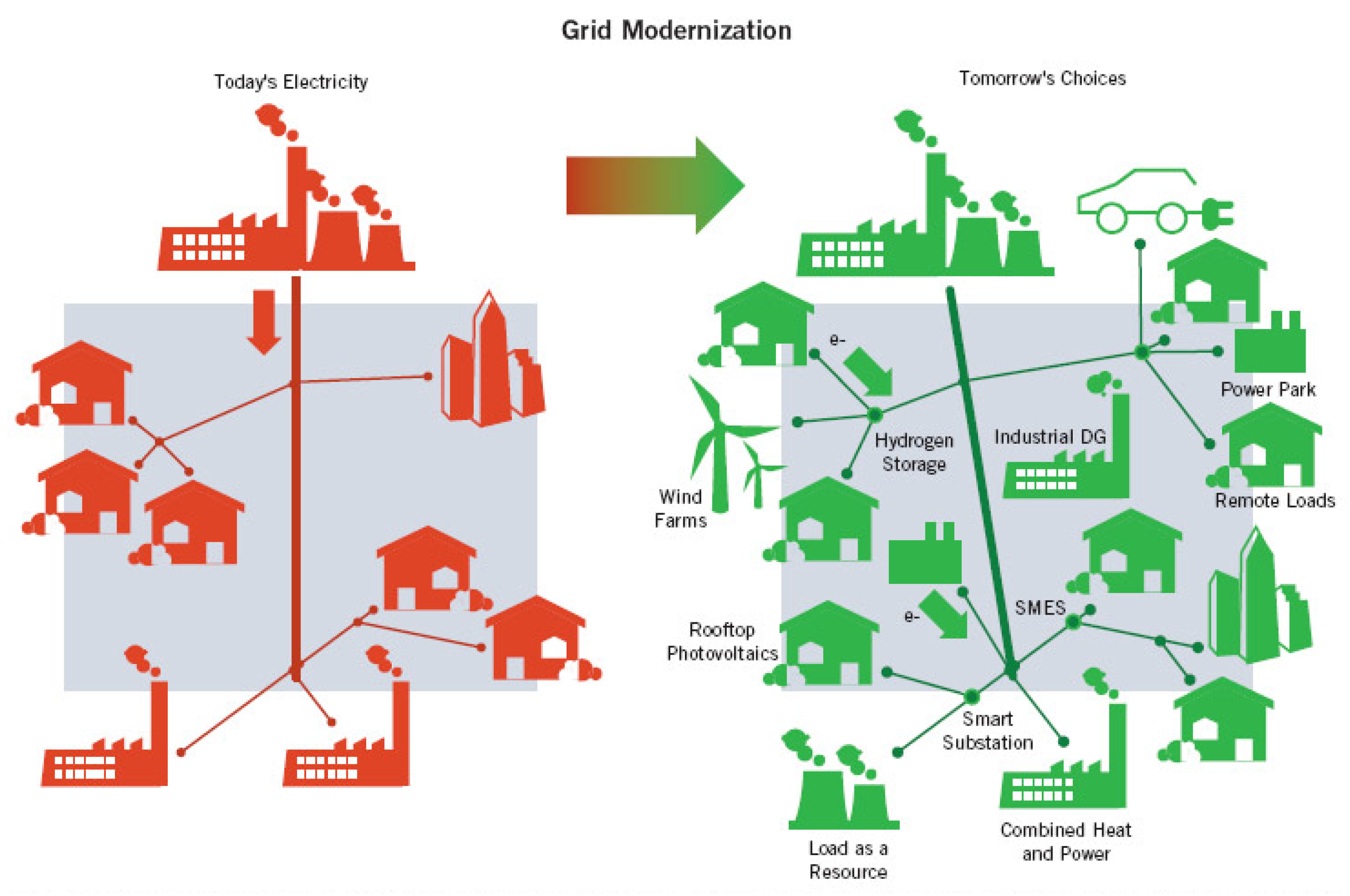
Figure 1 shows the distinctions between centralized systems and microgrids. There are other reasons for setting up microgrids; they reduce the cost of manufacturing, maintenance and operation, increase efficiency, reduce emissions, and improve energy quality [4]. Uncentralism implies an enhanced microgrid’s reliability and accessibility owing to distributed generators. Microgrids are usually incorporated and linked to renewable sources of energy. These sources are capable of making the system more economical than centralized systems based on standard generators. The operating cost decreases enormously when renewable energy sources are integrated with a microgrid. This is because the renewable power sources’ operating expenses are negligible compared to standard generators which depend on fuel expenses for their operating costs.

Renewable power is freely accessible, but it requires investment costs to transform renewable energy to electricity. The authors in [6] review renewable distributed generation unit integration techniques and methods in a distribution system. A storage system is one of the other significant parts that might be attached to a microgrid. There are many storage technologies that are quickly improving, and in microgrids there are many applications of them [7]. One of the significant applications, for example, is their contribution to supporting an emergency load. An ESS can also supply peaks with electrical energy [8].

The ESSs make electricity operation more economical and reduce expenses such as renewable energy sources. In addition, during low-price periods, electrical energy can be charged and stored. Moreover, during high-price periods they are able to discharge and supply the stored energy [1]. This method therefore leads to a more economic system that is less expensive to operate. Improve and boost the efficiency, reliability and accessibility of renewable energy sources and ESSs [9].

In addition, the Smart Energy Management System (SEMS) is a system used in a microgrid to coordinate various parts and devices [10]. These elements include renewable sources of electricity and ESSs. The SEMS has some goals and its main goal is to produce and create suitable set points for distinct sources and ESSs in order to minimize expenses and optimize energy dispatch or power distribution economically. A typical SEMS is shown in Figure 2 [11]. The authors in [12] propose a method for optimal dispatch of a microgrid that has ESSs.

Smart grids are a intelligent form of microgrids and are bi-directional energy and communication networks that enhance an electrical system’s reliability. They have all the phases observed in an electrical system and generation, transmission and distribution are those phases. They also have ESSs that considerably boost the efficiency of a power system. An ESS also reduces the total operating cost of a smart grid and saves a big part of the cost of fuel and maintenance [13]. Smart grids could be small-scale or large-scale systems. In addition, smart grids are green and generate much less emissions than traditional power systems.

Electric vehicles are regarded as ESSs. Like other ESSs, they charge and discharge. Before incorporating them into a microgrid, ESSs should be optimally sized [8]. Many methods are available to discover an ESS’ ideal size. The optimum size of the ESS is when this size minimizes the total investment and operating costs. 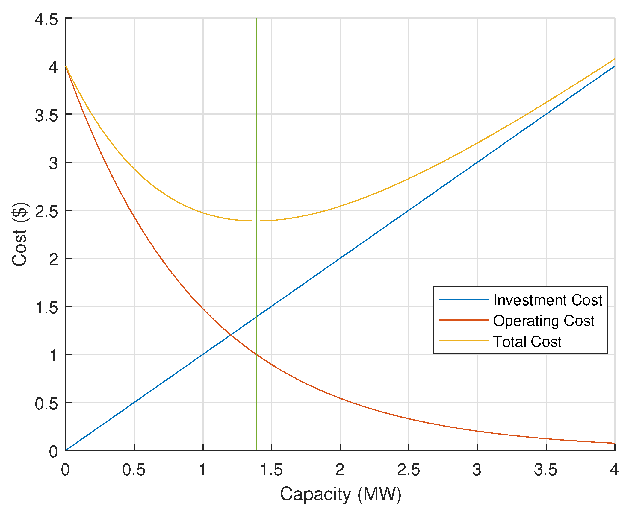Furthermore, the expenses and profits of exchanged energy are included in the total cost of in grid-connected microgrids [3]. There is a mathematical relationship between the size of an ESS and its cost of investment and its cost of operating microgrid. As the size rises, the investment cost increases linearly. However, as the size rises, the operation cost reduces exponentially [1]. The total cost is the sum of those two expenses. The goal is to calculate the size at the minimum total cost [14]. This connection is illustrated in Figure 3. The ESS should be at its optimum size because an over-sized ESS results in elevated investment costs whereas an undersized ESS may not be able to provide financial and operational advantages [1]. The authors in [15] suggest an ESS methodology for future autonomous systems to be optimally sized.

One of the optimization techniques is used to calculate the ideal size of an ESS. Some of these methods are mixed-integer linear programming (MILP) [8], mixed-integer non-linear programming (MINLP) [16], dynamic programming (DP) [17,18], particle swarm optimization (PSO) [19], two-stage stochastic programming [20], distributionally robust optimization [21], model predictive control (MPC) [22]. The optimization problems parameters may be either certain or uncertain. Deterministic methods of optimization are used with certain parameters to solve problems of optimization, while probabilistic methods are used to solve problems with unclear parameters. In addition, there are several algorithms to find the ideal size of an ESS in relation to optimization methods. A method has been suggested by the authors in [23] to optimally size a hybrid ESS (HESS). This HESS comprises of batteries and ultracapacitors that are rechargeable. In addition, the authors provided a methodology to optimize the joint ability of renewable energy and an HESS in [24].

Stochastic optimization or robust optimization are used to solve problems of optimization with uncertainty in their parameters [20]. Furthermore, the heuristic algorithm is also used to solve problems of probabilistic optimization. This algorithm and one of its applications in power system optimization were described by the authors in [25]. They used the algorithm to find in a microgrid the optimal functioning of distributed generators. 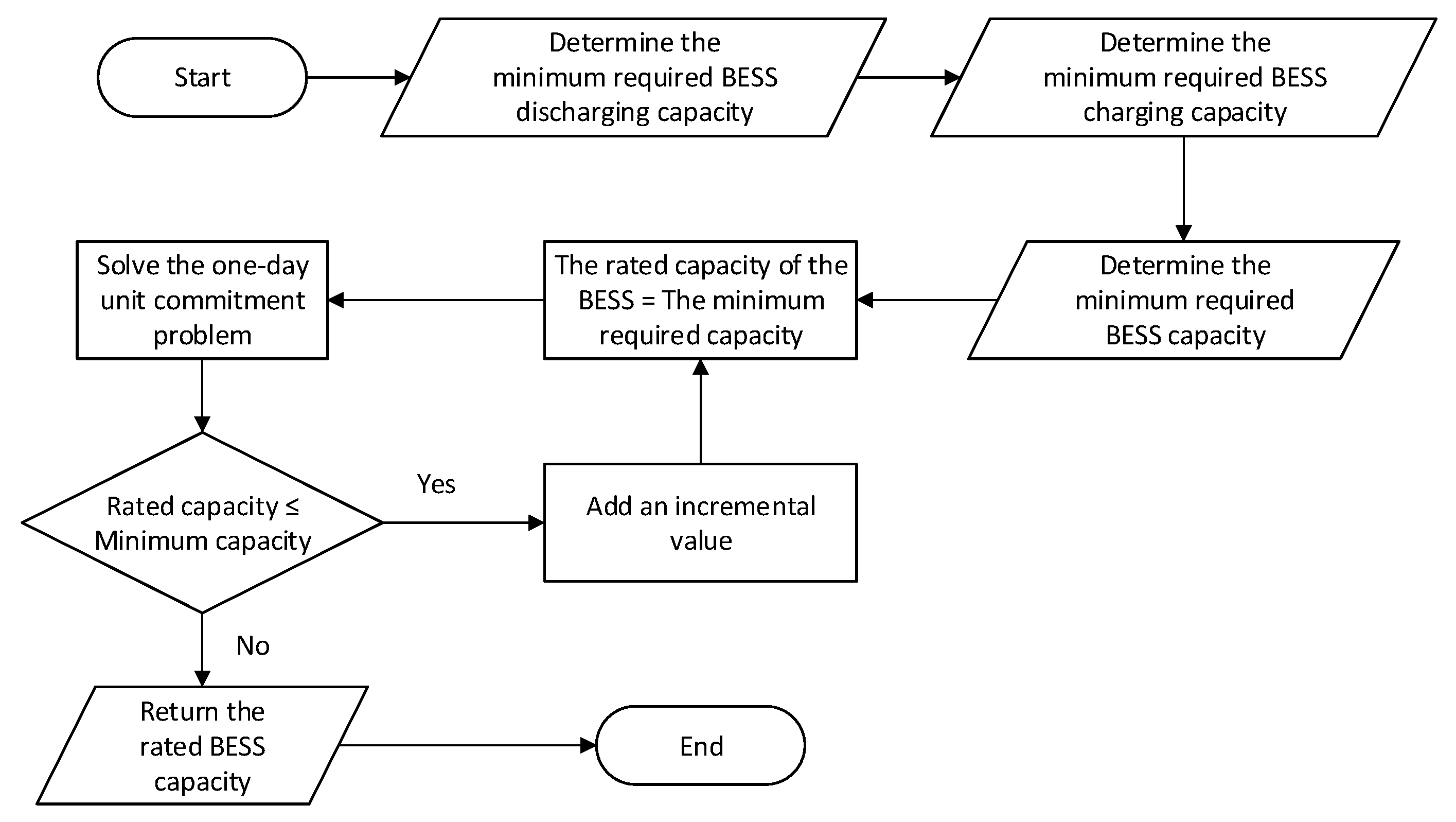In addition, the authors in [8] suggested an algorithm to optimally size a battery ESS (BESS) in an isolated microgrid. This algorithm’s goal is to discover the BESS size that minimizes the total cost. This algorithm is described in [8] in details. Figure 4 briefly demonstrates this method and algorithm and how it is used to size the BESS optimally.

The ESS is one of the very appealing alternatives for enhancing and improving microgrid scheduling and operation flexibility. This is because an ESS can also absorb energy when prices are low or excessive generation occurs. After that, when prices are high or when electricity is low, it returns this energy [26]. There are many technologies available for ESSs. Some of these techniques include superconductive magnetic energy storage (SMES) [27], compressed air storage (CAES) [28], supercapacitor energy storage [29], pumped hydro storage [30], battery energy storage (BESS) [31], flywheel energy storage [32], and gas storage process [33]. In [34], more ESS technologies are evaluated and analyzed.

Different objective features associated with an ESS are used in power system optimization [26]. Some of them compensate for grid voltage changes [27] and overcome the destabilizing impact of instant steady energy loads in DC microgrids [29]. Additionally, other objective features include preventing the shedding of transient under-frequency loads [35] and improving reliability [36]. In addition, there is wind uncertainty management [37] and fault rides through grid-connected assistance. In addition, offshore wind farms based on VSC HVDC [32], phase balancing [38], reduction of wind curtailment and congestion management [39] are objective functions. Minimization of active energy loss payment [40] is another objective function for optimizing ESSs. Additionally, in a power distribution system [41], ESSs could be optimized with other distributed generators.

Other microgrid-related optimization problems associated with ESSs include optimal planning. The authors in [42] are proposing a fresh ideal planning model to minimize the operating costs of an isolated microgrid that is not attached to a bigger grid using casual programming. Setting the confidence levels of the probability limitations of the spinning reserve results in microgrid operation through a trade-off between reliability and economy. The authors in [43] also suggest a fresh bi-level ideal planning model to promote the involvement of ESSs in the regulation of the isolated financial activity of microgrids. In this model, the upper-level sub-problem could be formulated to minimize the net cost of isolated microgrid, while the lower-level aims at maximizing ESS profits in real-time pricing environments that are determined in the upper-level decision by demand responses. In addition, a two-stage optimization technique is suggested in [44] for optimal distributed generation unit planning considering the inclusion of an ESS. The first phase uses the well-known loss sensitivity factor strategy to determine the places of the installation and the original capability of the distributed generation. In addition, the second phase defines the distributed generation’s ideal assembly capabilities for maximizing investment advantages and system voltage stability and minimizing line losses.

Due to the inclusion of renewable energy sources, ESSs are becoming increasingly important and have many applications [45]. Some generation must be accessible to keep system stability in order to use wind turbines to produce electricity. In this case, ESS can be used to avoid installation of fresh generation crops [46,47]. ESS can also store unusable electrical energy from wind turbines and photovoltaic cells. When a sudden shift happens, this energy can be used later. For example, during a sudden passage of dark clouds, ESS can support PV crops to restore voltage dip, resulting in a smooth output of [48,49]. Other ESS applications include improving power quality [50,51], emergency operating reserves [52,53], decreasing the likelihood of power blackouts [54], supply and demand matching [55], load shifting [56], transmission and distribution deferral upgrade [57], grid black start [58], energy arbitration [59], voltage support [60], frequency balancing [61,62] and conventional generation reduction during peak hours [63]. In addition, as shown in this paper, one of the most significant applications is to reduce operation and maintenance costs. ESSs have no rotating components, resulting in lower operating and maintenance costs and easier troubleshooting [64,65].

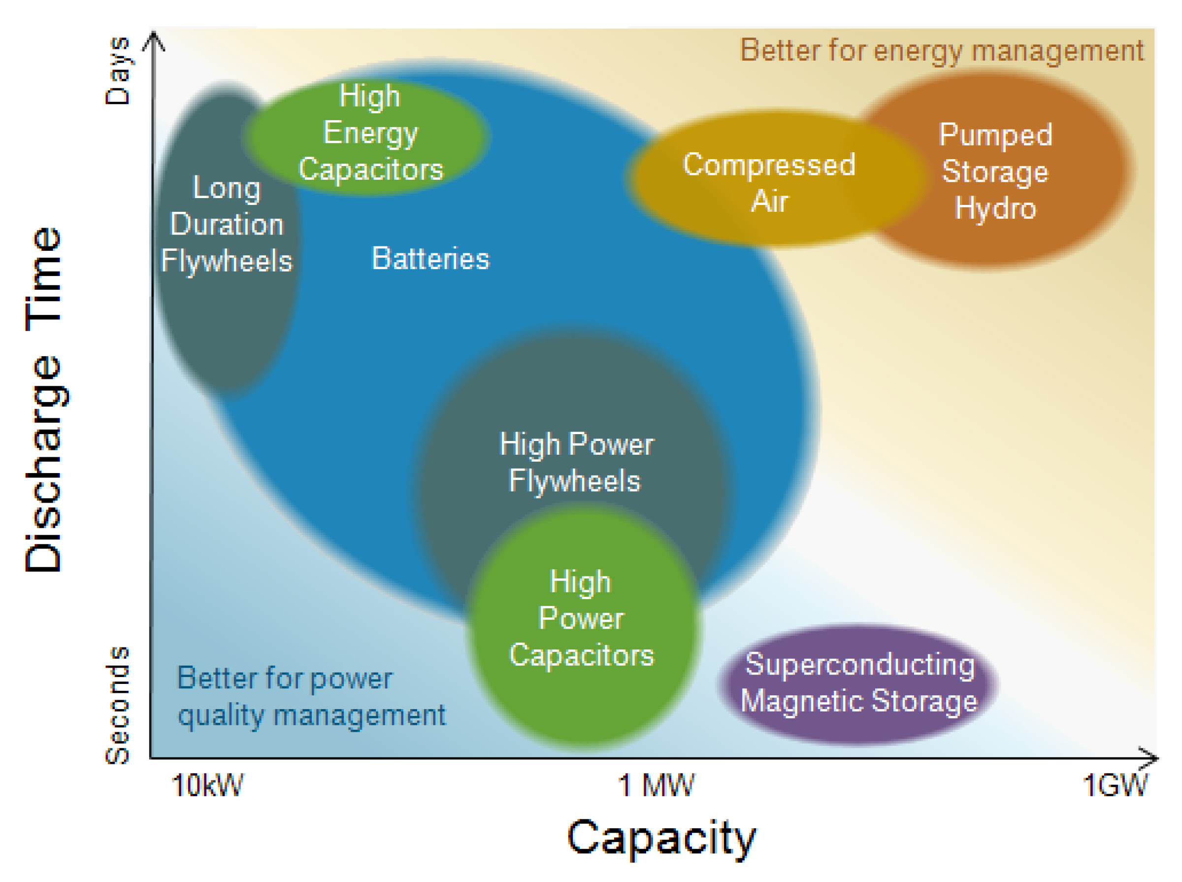
Various kinds of ESSs were intended and created. Some of these are already commercially accessible. The remainder of them still need to be enhanced in studies. There are distinct charging and discharge features of distinct ESS techniques. The charging and discharge rates among these distinct techniques are also distinct. Figure 5 shows various ESS technologies’ power and discharge rate. To compare the various ESS systems, several criteria are used. The authors in [66] contrasted various features and the benefits and disadvantages of ESS techniques. Reliability is a crucial factor in evaluating a certain power system. It is essential for both parties to evaluate the reliability of a power system; providers and clients. Reliability of a power system implies that the system should be accessible at an financial and sensible cost to supply electrical energy when it is required. In order to improve and boost the reliability of power systems, many techniques and devices have been created. In addition to the other benefits that an optimally sized ESS provides for a microgrid, ESSs enhance the reliability of the microgrid when integrated with it [67]. ESSs in many respects improve accessibility. One of them is that they are supporting demand shaving, particularly at peak times. In addition, it does not cost in terms of manufacturing or operation when an ESS is formed. There are other indexes of reliability and they also improve after the ESS has been integrated [3].

The uncertainty is important when renewable energy sources are integrated into a power system because the power output from these sources cannot be correctly determined. This also relies primarily on forecasts that are not entirely accurate. Furthermore, reliability is now becoming more important and many techniques are being created to improve reliability. The missing gap in the literature is that under wind uncertainties there is no technique for optimally sizing an ESS for a microgrid. The uncertainties must be taken into consideration in order to find the optimum size of an ESS for a microgrid linked to renewable energy sources. In this case, the problem is called a probabilistic problem of optimization that is distinct from deterministic problems of optimization. Two techniques used to optimize such problems are stochastic optimization and robust optimization. Stochastic programs are complicated and more hard to formulate [69]. There are many approaches to solving stochastic problems of optimization. Some of these approaches are breakdown, statistically based techniques, stochastic breakdown, multi-stage problem techniques and computational illustration [69]. The generic sizing methodology using pinch analysis and design room is another technique for optimally sizing an ESS linked to a system with renewable energy sources [70]. Benders decomposition is one of the decomposition methods used to solve very big stochastic optimization problems [71]. Benders decomposition is a method used with scenarios to solve stochastic programming problems.

3. Problem Formulation

The problem formulation is subdivided into Section 3.1 and Section 3.2. A detailed explanation about reliability assessment is in [72].

3.1. Optimal Sizing of an ESS

The model of one of the popular power system optimization problems is used to calculate the ideal size. This problem is the problem of unit commitment. In addition to the unit commitment problem, ESS constraints will be added and the solution will include the unit commitment solution and optimal size. The problem of unit commitment is discussed in [14,73]. Furthermore, ESS limitations to be added to the unit commitment model are described in [14]. The suggested problem of optimization was modeled and to solve the problem, a GAMS (General Algebraic Modeling System) code was created. The references [26,74] explain the development of GAMS codes.

3.1.1. Objective Function

Cost function is the objective function of the optimization problem. The goal is to minimize the overall cost. The total expense, therefore, involves the expenses of ESS investment, operation and exchanging energy with the main grid. In the following equation, the objective function of the optimal size problem for a specified horizon is developed.

$$minCM{G}_{units}+CM{G}_{ex}+I{C}_{ESS}$$

(1)

where $CM{G}_{units}$ is the operating cost of distributed microgrid generators, $CM{G}_{ex}$ is the cost or revenue of the exchanged power imported or exported from the main grid, and $I{C}_{ESS}$ is the investment cost necessary to establish the ESS.

The operation cost of microgrid distributed generators is calculated using the equation formulated in Equation (2). The decision variables u, y, and z are binary variables. This means that they have only two values which are either 1 or 0. If $u_{i,t}$ is 1, this means that the generator i at hour t is ON, and if it is 0, the generator is OFF. In addition, if $y_{i,t}$ is 1, this means the generator i starts up at hour t. In addition, if $z_{i,t}$ is 1, the generator i at hour t shuts down. So, the $y_{i,t}$ and $z_{i,t}$ are 1 during the first hour the generator starts up and shuts down, respectively. The values of $y_{i,t}$ and $z_{i,t}$ are 0 during the rest of the hours. Since the values of $u_{i,t}$, $y_{i,t}$ and $z_{i,t}$ are integers, MILP should be used to solve the optimization problem. The fixed cost of unit i, F, is fixed if the unit i is ON. This cost is calculated during all hours the unit is committed at. The output power of the unit does not matter in calculating the fixed cost. However, the variable cost of unit i, V, is variable and it is dependent on the output power of the unit i.

$$CM{G}_{units}=\sum _{t=1}^{NT}\sum _{i=1}^{NI}[F_i{u}_{i,t}+V_i{P}_{i,t}+S{U}_i{y}_{i,t}+S{D}_i{z}_{i,t}]$$

(2)

where i is the unit index, $NI$ is the number of units, t is the hour index, $NT$ is the number of hours, $F_i$ is the fixed cost or no-load cost of unit i, $V_i$ is the variable cost of unit i and it is related to the output power of unit i, $P_{i,t}$ is the output power of unit i at hour t, $S{U}_i$ is the start up cost of unit i and $S{D}_i$ is the shut down cost of unit i. $u_{i,t}$, $y_{i,t}$, and $z_{i,t}$ are binary variables represent the commitment state of unit i at hour t, start up indicator of unit i at hour t and shut down indicator of unit i at hour t, respectively.

A nonlinear quadratic function is used as a cost function to calculate the generator’s production cost. In Equation (2), however, it has been linearized to simplify and speed up modeling and solving the optimization problem. The quadratic function could be used for more precise outcomes in the objective function.

The following equation demonstrates how the cost of imported energy from the main grid or exported energy income to the main grid can be calculated. This cost is positive when energy is imported as the cost. Therefore, when electricity is exported to the main grid, the cost is negative.

$$CM{G}_{ex}=\sum _{t=1}^{NT}\gamma P_{M_t}$$

(3)

where $\gamma$ is electricity per one megawatt of power imported from or exported to the main grid and $P_{M_t}$ is the exchanged power between the microgrid and main grid at hour t. The sign convention in $P_{M_t}$ is that it is positive when the power flows from the main grid to the microgrid (imported) and it is negative when the power flows from the microgrid to the main grid (exported).

In the following equation, the investment cost of the ESS is expressed. The unit prices of ESS power and energy are the parameters in this equation. In addition, the decision variables are the ESS’s rated power and energy. These two variables constitute the optimum ESS size needed.

$$I{C}_{ESS}=P{C}_{ESS}{P}_{ESS}^R+E{C}_{ESS}{E}_{ESS}^R$$

(4)

where $P{C}_{ESS}$ is the power cost of the ESS per one megawatt, $P_{ESS}^R$ is the rated power of the ESS, $E{C}_{ESS}$ is the energy cost of the ESS per one megawatt hour and $E_{ESS}^R$ is the rated energy of the ESS.

3.1.2. System Constraints

System limitations include limitations on generators and equations for equilibrium. The equation of the equilibrium is an significant constraint because at the same moment the energy produced must be equivalent to the load. If the produced energy exceeds the load, the frequency of the system will increase. Furthermore, if the energy produced is less than the load, the frequency of the system will decrease. This variation is the frequency of the system might collapse or lead to a blackout. For this reason, the yield energy from generators, wind power and discharge energy from the ESS must be equal to the charging power of the load and the ESS. The Coordinated Frequency Framework for optimization is proposed by [75]. Reserve is sometimes added to the constraint so that the power generated is equal to the load and reserve. To be available when the load varies, the reserve is added to the balance equation, so that the output power must be equal to the sum of demand and reserve at each hour. Furthermore, the emission limit could also be added to some optimization problems [76]. In multi-objective unit commitment problems, the goals could be to simultaneously minimize costs and emissions [26]. The balance constraint is formulated in this paper as follows:

$$\sum _{i=1}^{NI}[P_{i,t}+P_{ES{S}_t}+P_{M_t}-\sum _{s=1}^{NS}{\rho }_s{P}_{W_{t,s}}]=D_t\forall t\in T,\forall s\in S$$

(5)

where s is the scenario index, $NS$ is the number of scenarios, ${\rho }_s$ is the probability of scenario s, S is the set of scenarios, $P_{ES{S}_t}$ is the power stored to or produced by the ESS at hour t, $P_{W_t,s}$ is the wind power at hour t in scenario s, $D_t$ is the demand at hour t and T is the set of hours. The sign convention in $P_{ES{S}_t}$ is that it is positive when it is produced (discharging case) and negative when it is stored (charging case).

Wind power is calculated from wind speed and it is calculated as illustrated below [7].

$$P_{W_{t,s}}=\left\{\begin{array}{cc}0\hfill & v_{t,s}<v_{CI}or{v}_{t,s}\ge v_{CO}\hfill \\ P_W^{max}\frac{v_{t,s}-v_{CI}}{v_R-v_{CI}}\hfill & v_{CI}\le v_{t,s}<v_R\hfill \\ P_W^{max}\hfill & v_R\le v_{t,s}<v_{CO}\hfill \end{array}\right.$$

(6)

where $P_W^{max}$ is the rated wind power, $v_{t,s}$ is the wind speed at hour t in scenario s, $v_{CI}$ is the cut-in wind speed, $v_{CO}$ is the cut-out wind speed and $v_R$ is the rated wind speed. Figure 6 shows how the output wind power changes with wind speed [77].

Due to the limit of the transmission line linking the two structures, the exchange capacity between the main grid and microgrid is restricted. To restrict this energy, a constraint is required, and it depends on the transmission line’s ability. When energy is transferred, the energy exchanged is negative and positive when it is transferred from the main grid. This limitation is formulated as follows:

$$-P_M^{max}\le P_{M_t}\le P_M^{max}\forall t\in T$$

(7)

where $P_M^{max}$ is the maximum capacity, limit, of the transmission line connecting between the microgrid and main grid.

There are distinct features of distinct generators. These features have certain limitations, such as peak energy. These limits are developed as limitations to be included in the problem of optimization. Generators have minimum boundaries to ensure that they are stable. In addition, because there is a maximum limit, each generator cannot have infinite energy. This constraint is formulated in the following equation. Minimum and maximum limits must be multiplied by $u_{i,t}$, the commitment state of a generator i at hour t. This is because if a generator is OFF, the output must be zero. The output power will have values all the time if the state does not multiply the limits as the output power should always be between the minimum and maximum limits.

$$P_i^{min}{u}_{i,t}\le P_{i,t}\le P_i^{max}{u}_{i,t}\forall i\in I,\forall t\in T$$

(8)

where $P_i^{min}$ is the minimum power that can be produced by unit i, $P_i^{max}$ is the maximum power that can be produced by unit i and I is the set of units.

Ramp up and ramp down boundaries are two factors that limit the rate of a generator’s output power to increase and decrease. A certain generator’s output power cannot be improved or voluntarily reduced. To represent these two boundaries, a restriction must be developed. The following equation formulates this limitation.

$$P_{i,t}-P_{i,t-1}\le R{U}_i\forall i\in I,\forall t\in T$$

(9)

where $R{U}_i$ is the ramp up rate of unit i.

$$P_{i,t-1}-P_{i,t}\le R{D}_i\forall i\in I,\forall t\in T$$

(10)

where $R{D}_i$ is the ramp down rate of unit i.

When a generation system begins running, ON, it has to run for a while before it shuts down. This period is referred to as the minimum uptime. Moreover, if a generation system shuts down, it must be OFF for a period of time before it begins. This period is referred to as the minimum downtime. These two limitations are set out below.

$$T_{i,t}^{ON}\ge MU{T}_i[u_{i,t}-u_{i,t-1}]\forall i\in I,\forall t\in T$$

(11)

where $T_{i,t}^{ON}$ is the ON time of unit i at hour t and $MU{T}_i$ is the minimum up time of unit i.

$$T_{i,t}^{OFF}\ge MD{T}_i[u_{i,t-1}-u_{i,t}]\forall i\in I,\forall t\in T$$

(12)

where $T_{i,t}^{OFF}$ is the OFF time of unit i at hour t and $MD{T}_i$ is the minimum down time of unit i.

Logically, the unit generation cannot begin and shut down simultaneously. It is possible to model this logic constraint as shown in the following equation.

$$y_{i,t}-z_{i,t}=u_{i,t}-u_{i,t-1}\forall i\in I,\forall t\in T$$

(13)

3.1.3. Energy Storage System Constraints

ESS restrictions restrict an ESS’ charging and discharging capabilities. Its rated power, which is the ideal size, limits the ESS power. More than its rated power, the ESS cannot charge or discharge. When charging, the ESS functions as a load and when it discharges acts as a generator. It is also presumed that the charging power is negative, whereas it is presumed that the discharge power is positive. This limitation is formulated as follows:

$$-P_{ESS}^R\le P_{ES{S}_t}\le P_{ESS}^R\forall t\in T$$

(14)

The energy stored in the ESS is limited by its rated energy, an output from the problem of optimization. The energy that is stored is always positive. This limitation is formulated as follows:

$$0\le E_{ES{S}_t}\le E_{ESS}^R\forall t\in T$$

(15)

where $E_{ES{S}_t}$ is the energy stored in the ESS at hour t.

The equation for calculating the charging status at a particular hour is formulated in (16). Charging status is the stored energy and techniques are established to optimize it [78].

$$E_{ES{S}_t}=E_{ES{S}_{t-1}}-P_{ES{S}_t}\forall t\in T$$

(16)

3.2. Reliability Indices

There is a statistical way to calculate the availability of a component or system and it is the probability of time that the component or system will be available during it. The unavailability, as defined in Equation (17), is the remaining probability.

$$U=1-A$$

(17)

where U is the unavailability and A is the availability.

The availability and unavailability are calculated from the mean time to fail (MTTF) of a component or system and the mean time to repair (MTTR) of a component or system as formulated in Equations (18) and (19), respectively.

$$A=\frac{MTTF}{MTBF}$$

(18)

where $MTTF$ is the mean time to fail and $MTBF$ is the mean time between failures.

$$U=\frac{MTTR}{MTBF}$$

(19)

where $MTTR$ is the mean time to repair.

The mean time between failures of a component or system is calculated as formulated in (20).

$$MTBF=MTTF+MTTR$$

(20)

In addition, the failure and repair rates are used to calculate the availability and unavailability as formulated in Equations (23) and (24), respectively.

$$\lambda =\frac{1}{MTTF}$$

(21)

where $\lambda$ is the failure rate.

$$\mu =\frac{1}{MTTR}$$

(22)

where $\mu$ is the repair rate.

These equations give Equations (23) and (24).

$$A=\frac{\mu }{\lambda +\mu }$$

(23)

$$U=\frac{\lambda }{\lambda +\mu }$$

(24)

In the system studied in the case study of this paper, the generation units, wind turbine and ESS are linked in parallel as shown in Figure 7 which shows only the generators and the parallel linked ESS. The equations used to calculate reliability indices of a system with only two parts will be obtained in the following equations. In addition, it is possible to derive equations of any comparable system with more than two parallel parts in the same manner. In addition, the equivalent or total unavailability for parallel connected components in a system is equal to the summation of all individual unavailability as formulated in Equation (25).

$$U_{sys}=U_1{U}_2$$

(25)

So, the equivalent availability is calculated as formulated in Equation (26).

$$A_{sys}=1-U_{sys}$$

(26)

In more details:

$$A_{sys}=1-U_1{U}_2$$

(27)

$$A_{sys}=1-\frac{MTT{R}_1}{MTT{F}_1+MTT{R}_1}·\frac{MTT{R}_2}{MTT{F}_2+MTT{R}_2}$$

(28)

Using the failure and repair rates:

$$U_{sys}=\frac{{\lambda }_1{\lambda }_2}{({\lambda }_1+{\mu }_1)({\lambda }_2+{\mu }_2)}$$

(29)

$$A_{sys}=1-\frac{{\lambda }_1{\lambda }_2}{({\lambda }_1+{\mu }_1)({\lambda }_2+{\mu }_2)}$$

(30)

To calculate the total repair and failure rates:

$${\mu }_{sys}={\mu }_1+{\mu }_2$$

(31)

$$U_{sys}=\frac{{\lambda }_1{\lambda }_2}{({\lambda }_1+{\mu }_1)({\lambda }_2+{\mu }_2)}$$

(32)

$$\frac{{\lambda }_{sys}}{{\lambda }_{sys}+{\mu }_{sys}}=\frac{{\lambda }_1{\lambda }_2}{({\lambda }_1+{\mu }_1)({\lambda }_2+{\mu }_2)}$$

(33)

$${\lambda }_{sys}=\frac{{\mu }_{sys}{\lambda }_1{\lambda }_2}{{\mu }_1{\mu }_2+{\lambda }_1{\mu }_2+{\lambda }_2{\mu }_1}$$

(34)

Which yields to:

$${\lambda }_{sys}=\frac{({\mu }_1+{\mu }_2){\lambda }_1{\lambda }_2}{{\mu }_1{\mu }_2+{\lambda }_1{\mu }_2+{\lambda }_2{\mu }_1}$$

(35)

Simply, calculating the corresponding MTTF and MTTR are shown in Equations (36) and (37).

$$MTT{F}_{sys}=\frac{1}{{\lambda }_{sys}}$$

(36)

$$MTT{R}_{sys}=\frac{1}{{\mu }_{sys}}$$

(37)

The reliability indices are calculated as:

$$SAIDI=\frac{Totaldurationofallinterruptions}{Totalnumberofcustomersconnected}$$

(38)

$$SAIDI=\frac{{\displaystyle \sum _{i=1}^n}{r}_i{N}_i}{N_T}$$

(39)

$$SAIFI=\frac{Totalnumberofallinterruptions}{Totalnumberofcustomersconnected}$$

(40)

$$SAIFI=\frac{{\displaystyle \sum _{i=1}^n}{N}_i}{N_T}=\frac{{\displaystyle \sum _{i=1}^n}{\lambda }_{LP}{N}_{LP}}{N_T}$$

(41)

$$CAIDI=\frac{Totaldurationofallinterruptions}{Totalnumberofallinterruptions}$$

(42)

$$CAIDI=\frac{{\displaystyle \sum _{i=1}^n}{r}_i{N}_i}{N_T}=\frac{SAIDI}{SAIFI}$$

(43)

3.3. Uncertainty Modeling

Multiple wind speed profiles will be produced to model the wind uncertainty. These profiles will be given different probabilities and the summary of these probabilities must be equivalent to 1. Then, with its respective wind velocity profile, each likelihood is increased. The summation of these products will create a fresh profile to be used to solve the optimum problem of sizing. This solution will be contrasted with each profile’s solution to justify solving the problem using this technique when the optimization problem is uncertain. In Algorithm 1, the methodology for optimum sizing under wind uncertainty is demonstrated and simplified.

Algorithm 1 Calculating the solution after averaging the inputs.

1:  function SP_Sizing($n,S,P$) ▹ Where n—number of scenarios, S—array of all scenarios, P—vector of all scenario probabilities

2:   n = number of scenarios

3:   for $i=1$ to n do

4:     $S\left[i\right]$ = scenario profile

5:     $P\left[i\right]$ = scenario probability

6:   end for

7:   if ${\displaystyle \sum _{i=1}^n}P\left[i\right]>1$ then

8:     print: sum of probabilities is greater than 1

9:     Stop

10:   else

11:     $A={\displaystyle \sum _{i=1}^n}P\left[i\right]S\left[i\right]$     ▹ Where A—vector of scenarios multiplied by their corresponding probabilities

12:   end if

13:   for $i=1$ to n do

14:     Optimally size $S\left[i\right]$

15:   end for

16:   Optimally size A

17:   Compare the results

18:  end function

Another method is also used to calculate an ESS’ optimum size under uncertain wind conditions. This method’s algorithm is shown in the Algorithm 2. This technique could provide a more economical solution. Thus, in this technique, the optimally sized ESS could cost less than the technique originally suggested.

Algorithm 2 Calculating the solution after averaging the outputs.

1:  function SP_Sizing($n,S,Pr$)    ▹ Where n—number of scenarios, S—array of all scenarios, $Pr$—vector of all scenario probabilities

2:   n = number of scenarios

3:   for $i=1$ to n do

4:     $S\left[i\right]$ = scenario profile

5:     $Pr\left[i\right]$ = scenario probability

6:   end for

7:   if ${\displaystyle \sum _{i=1}^n}Pr\left[i\right]>1$ then

8:     print: sum of probabilities is greater than 1

9:     Stop

10:   else

11:     Find $P_{ESS}\left[i\right]$    ▹ Where $P_{ESS}\left[i\right]$—optimally sized ESS power for all scenarios separately

12:     Find $E_{ESS}\left[i\right]$   ▹ Where $E_{ESS}\left[i\right]$—optimally sized ESS energy for all scenarios separately

13:     $P^{ESS}={\displaystyle \sum _{i=1}^n}{P}_{ESS}\left[i\right]Pr\left[i\right]$       ▹ Where $P^{ESS}$—normalized optimal size ESS power

14:     $E^{ESS}={\displaystyle \sum _{i=1}^n}{E}_{ESS}\left[i\right]Pr\left[i\right]$      ▹ Where $E^{ESS}$—normalized optimal size ESS energy

15:   end if

16:   for $i=1$ to n do

17:     Optimally size $S\left[i\right]$

18:   end for

19:   Compare the results

20:  end function

3.4. Reliability Constraints

In order to ensure less interruptions and unavailability, some reliability limitations are implemented. The reliability limitations suggested in this paper are as shown in Equations (44) and (45).

$$SAIFI\le SAIF{I}_{Limit}$$

(44)

$$SAIDI\le SAID{I}_{Limit}$$

(45)

4. A Case Study

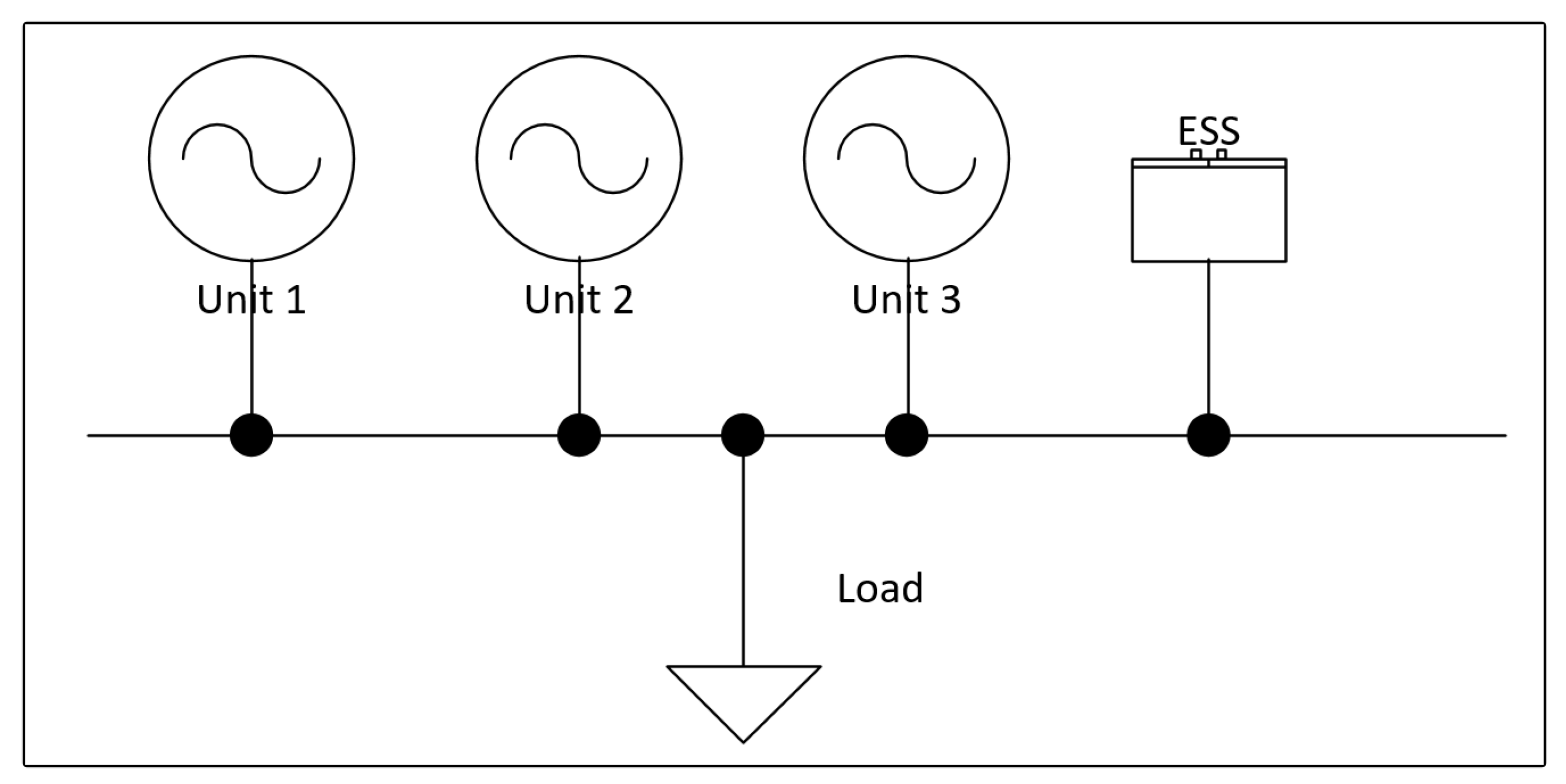
A microgrid linked to a main grid is regarded to conduct a case study in order to optimally size an ESS under wind uncertainties and to calculate the reliability indices. The case study will be provided with its information in this chapter. The findings will be presented and discussed in Section 5. The system to be studied is made up of three heat generators distributed in the microgrid. The problem of unit commitment is solved using stochastic programming for a two-year planning horizon. For the first year, the load information was drawn from the IEEE Reliability Test System (RTS-96) [79]. The same load profile was repeated with a rise of %5 for the second year. In this case research, reserve and emission limitations are not regarded. Weibull distribution uses Dhahran city’s Weibull distribution parameters to create wind speed scenarios. From historical information, these parameters were calculated. Since there is uncertainty and wind speed cannot be predicted accurately, the uncertainty and randomness should be dealt with in many scenarios. In this paper, fresh scenarios were produced using the parameters instead of taking scenarios from historical information. One of the techniques used to manage randomness in stochastic optimization is to consider distinct situations. Ten wind speed scenarios were developed randomly using the Weibull distribution parameters calculated for 19 years in Dhahran for monthly wind distribution [80].

Table 1. Weibull parameters for monthly wind speed distribution in Dhahran.

Month	k	c
JAN	2.40	4.77
FEB	2.45	4.85
MAR	2.55	5.15
APR	2.40	5.06
MAY	2.40	5.52
JUN	2.60	6.51
JUL	2.50	5.54
AUG	2.30	4.91
SEP	2.20	4.18
OCT	2.05	4.09
NOV	2.20	4.38
DEC	2.00	4.68

shows these parameters. In this table, K is the parameter of the form and c is the parameter of the scale. The Weibull distribution’s probability density function used to calculate each hour’s wind speed is formulated in Equation (46). It is presumed that these ten scenarios are real information collected from ten distinct years. It is presumed that the real information from ten years is taken. The annual number values of k and c are respectively $2.35$ and $4.98$. 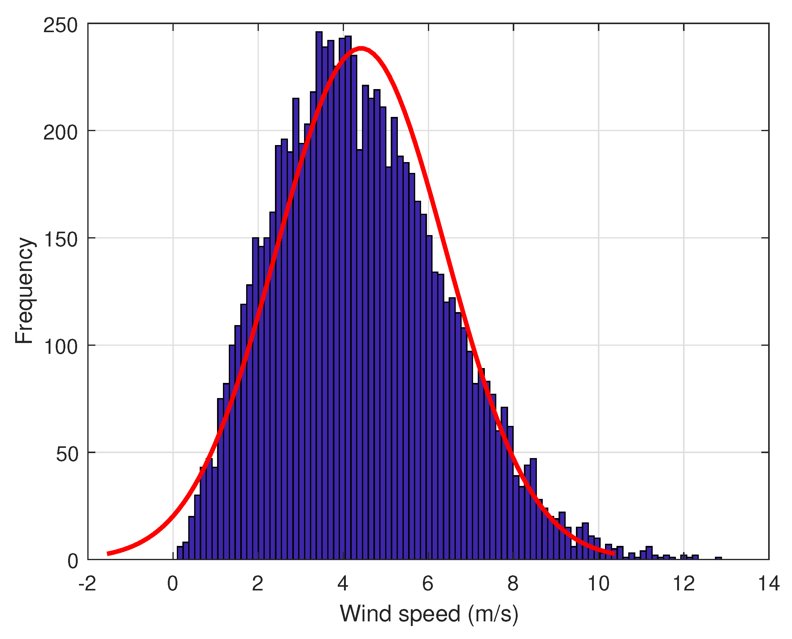Figure 8 indicates the Weibull distribution for annual wind speeds and the Dhahran wind frequency histogram [80] and

Table 2. Average annual wind speeds in Dhahran for all scenarios.

Scenario	Wind Speed (m/s)
Scenario 1	4.4446376
Scenario 2	4.4169281
Scenario 3	4.4102231
Scenario 4	4.4032716
Scenario 5	4.4007090
Scenario 6	4.4340644
Scenario 7	4.3894760
Scenario 8	4.3762805
Scenario 9	4.4285103
Scenario 10	4.3670960

shows the average annual wind speeds for all situations in Dhahran. All scenario probabilities are equivalent, meaning that for all cases, ${\rho }_s$ is equivalent to $0.1$. The ten scenarios were repeated for a second year to cover the two-year horizon.

$$f(t,c,k)=\left\{\begin{array}{cc}\frac{k}{c}{\left(\frac{t}{c}\right)}^{k-1}{e}^{-{\left(\frac{t}{c}\right)}^k}\hfill & t\ge 0\hfill \\ 0\hfill & t<0\hfill \end{array}\right.$$

(46)

The features of the three generation units are shown in

Table 3. Characteristics of generation units.

Unit No.	Fixed Cost	Variable Cost	Start Up	Shut Down	Min. Capacity
	($)	($/MW)	Cost ($)	Cost ($)	(MW)
1	9	20	40	20	5
2	7	18	30	20	3
3	5	15	20	20	2
Unit No.	Max. Capacity	Ramp Down	Ramp Up	Min. Down	Min. Up
	(MW)	Rate (MW/h)	Rate (MW/h)	Time (h)	Time (h)
1	20	15	15	1	1
2	30	15	15	1	1
3	40	20	20	1	1

. Except for the minimum uptime and minimum downtime, the generation unit features are from [73]. The reliability indices are calculated before the optimally sized ESS is integrated and the impact of integrating an optimally sized ESS on the reliability of the microgrid is investigated after its integration. In these calculations, the component $MTTF$ and $MTTR$ are required and displayed in

Table 4. Mean time to fail ($MTTF$) and mean time to repair ($MTTR$) of system components.

Component	$\mathit{MTTF}$	$\mathit{MTTR}$
	(hr/year)	(hr/year)
Unit 1	1200	15
Unit 2	1100	35
Unit 3	400	25
Wind Turbine	1477.7	25
ESS	150	15

.

Table 5. Values of other model parameters.

Parameter	${\mathit{PC}}_{\mathit{ESS}}$	${\mathit{EC}}_{\mathit{ESS}}$	$\mathit{\gamma }$	${\mathit{P}}_{\mathit{M}}^{\mathit{max}}$	${\mathit{SAIFI}}_{\mathit{Limit}}$
Value	$1200	$300	$20	10 MW	1.00 × 10${}^{-10}$
Parameter	$P_W^{max}$	$v_{CI}$	$v_R$	$v_{CO}$	$SAID{I}_{Limit}$
Value	15 MW	1 m/s	5 m/s	11 m/s	1.00 × 10${}^{-10}$

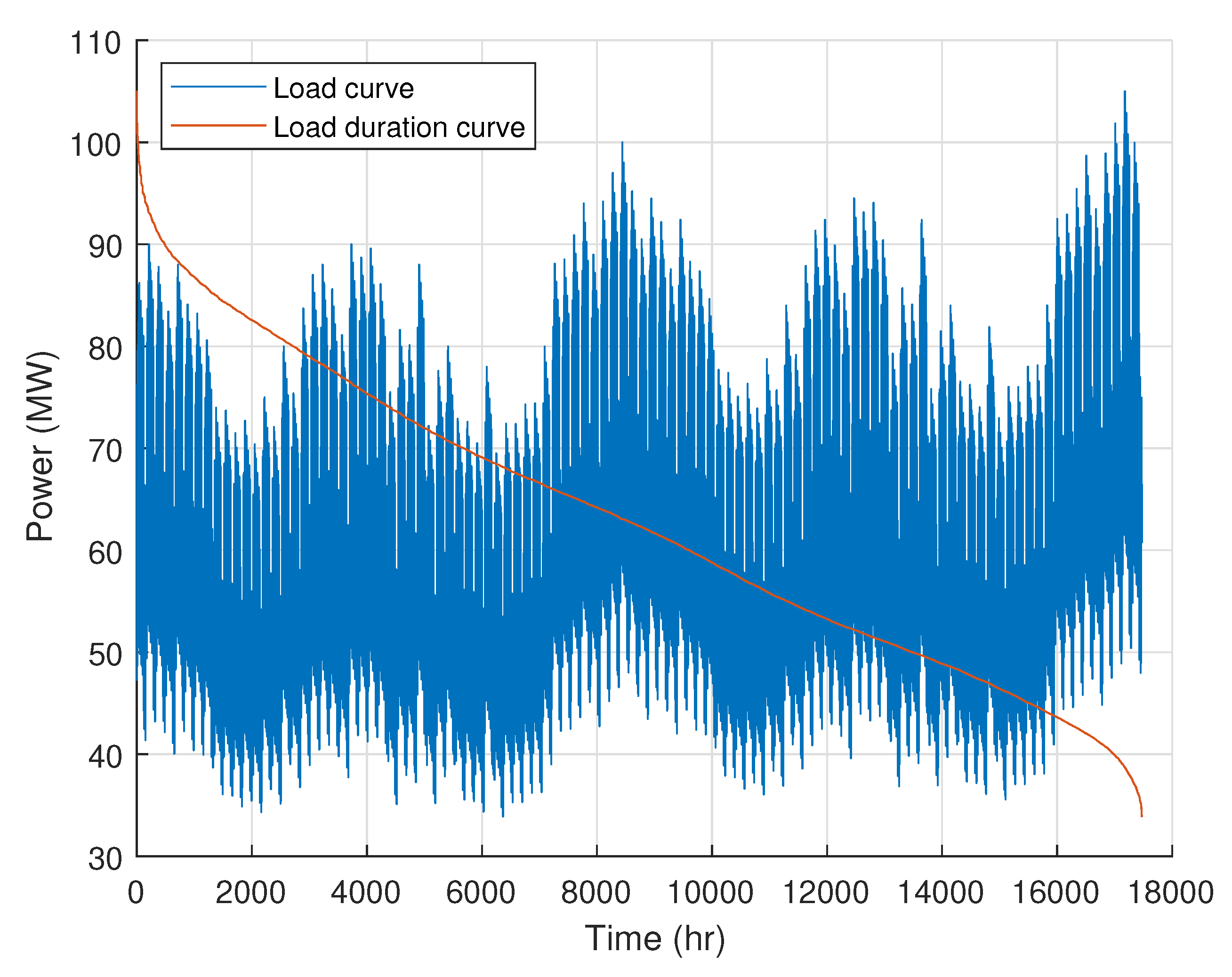
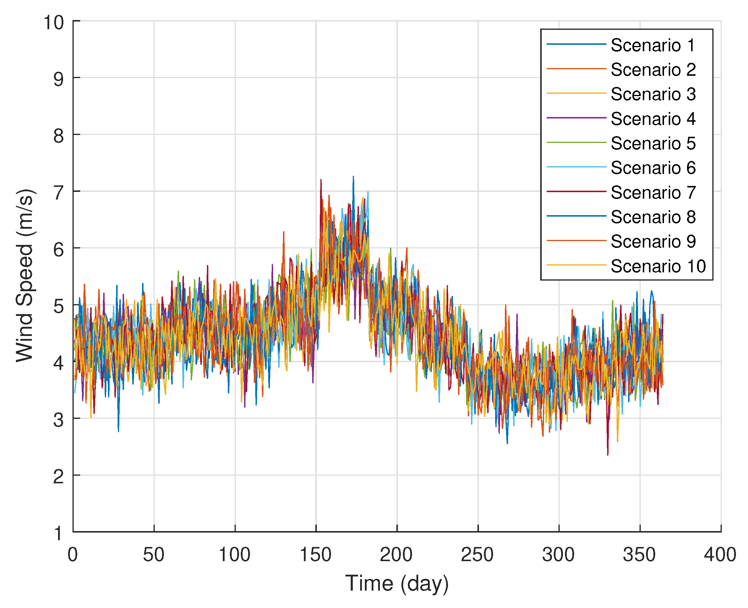
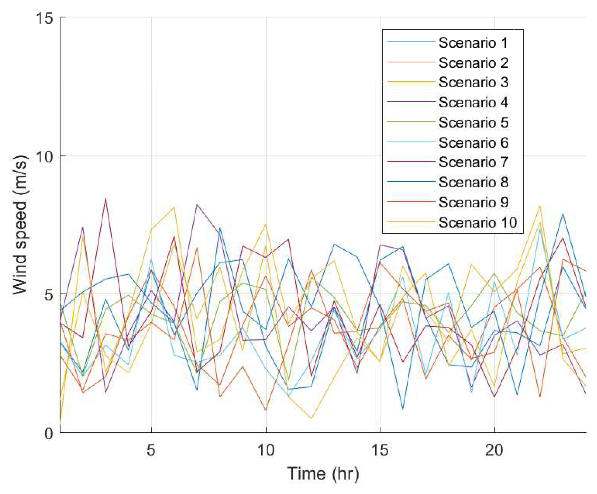
reflects the values used in this model for the other parameters. Figure 9 demonstrates the load curve over the two years as well as the load duration curve. Figure 10 demonstrates the first year’s ten wind velocity scenarios. They are depicted at daily average speeds. Repeat the same situations again to cover the second year. Figure 11 shows the hourly velocity of the first twenty-four hours for the ten situations.

The microgrid unit commitment problem is solved for a two-year horizon before and after the integration of the ESS to calculate the output power of each generation unit, the power exchanged with the main grid, and the power taken or produced in the second case by the ESS. The total cost of investment and generation will also be explored in relation to the reliability indicators. This system’s optimization problem was modeled in the language of GAMS (General Algebraic Modeling System) [81] and was solved in the NEOS server [82], a free online service to solve numerical optimization problems.

5. Results and Discussions

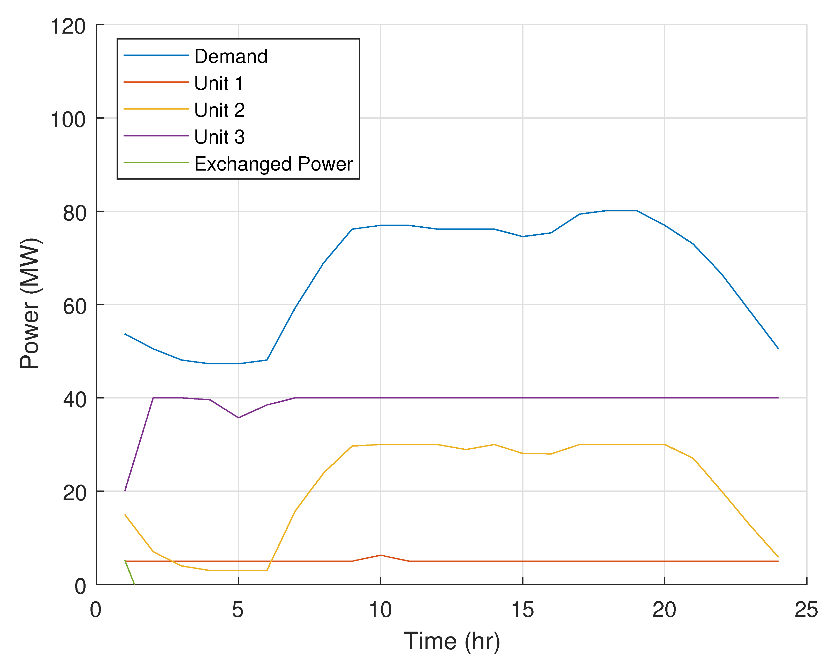
The problem of unit commitment was solved using the stochastic programming method to find the optimal size of the ESS that minimizes total cost. The ESS has been discovered to have a rated power of 16.59 MW and the rated power is 128.84 MWh. The ESS’ investment cost is approximately $58,554. 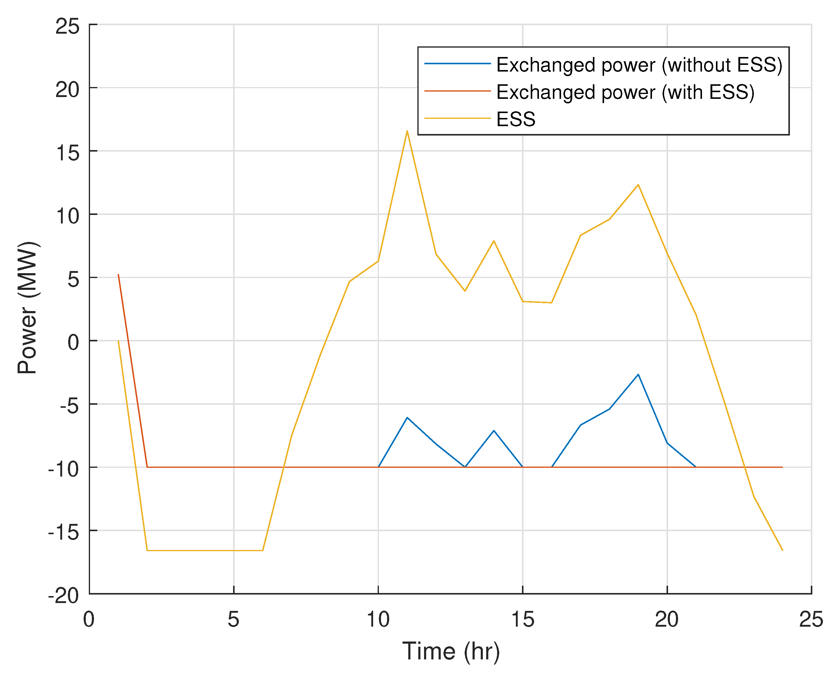Figure 12 demonstrates the unit commitment problem solution for the first twenty-four hours before combining the microgrid with the ESS and Figure 13 demonstrates the unit commitment problem solution after calculating the ideal size of the ESS and integrating it with the microgrid. These two numbers only depict the power with favorable values, meaning that they do not represent the power when charging the ESS and also when selling power to the main grid. 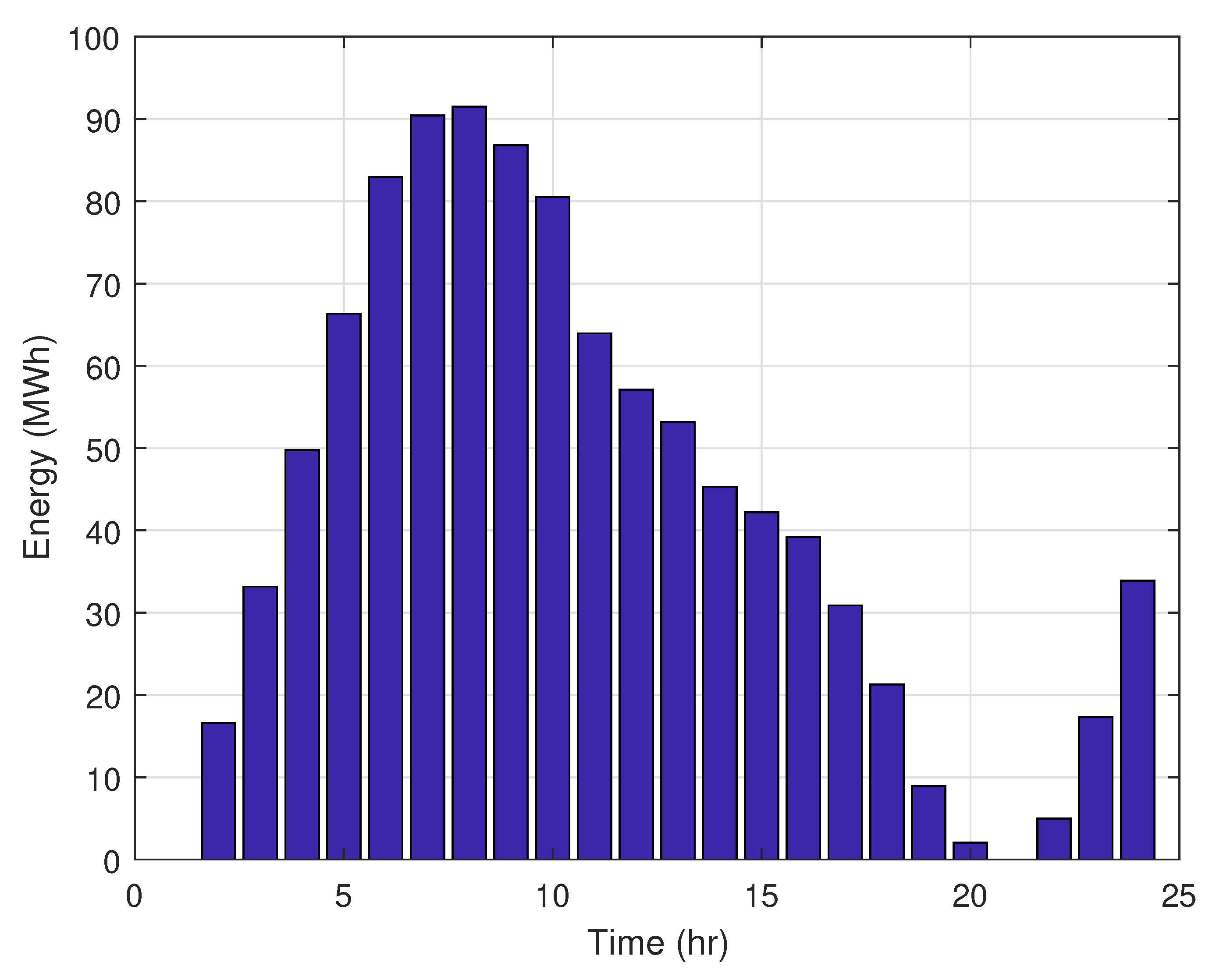The two variables associated with the energy generated by the ESS and the power exchanged with the main grid are shown with their adverse values in Figure 14. The ESS functions as a load when charging and when it discharges acts as a generator. The same concept is applied to the main grid where, when energy is imported into the microgrid, it is considered as a load when energy is exported to the microgrid. The ESS and central grid are the only elements that, due to the bidirectionality of the energy in these parts, have authority with negatives. It must have stored energy in order for the ESS to generate power. Figure 15 indicates the amount of energy collected during the first twenty-four hours.

The most expensive generation unit, which is Unit 1, is working at a low level when the ESS in not integrated as shown in Figure 12 and it is not working for most hours when the ESS is integrated as shown in Figure 13 in order to reduce the operation cost. The ESS has made the microgrid more reliable economically and saved a portion of the production cost when it worked instead of Unit 1. Figure 12 and Figure 13 show the solutions of the unit commitment problem in both cases as mentioned previously. By solving the unit commitment problem, it is required to match energy demand at the minimum cost. As shown in Figure 13, it is noticeable that the most expensive unit is OFF for most of the time and the demand is supplied at a lower cost because of the optimally sized ESS. The cost function of a unit is assumed to be linear in this case study. This leads to differentiate and sort the units by cost easily. The cheapest unit runs first and then the second cheapest and so on till matching the demand.

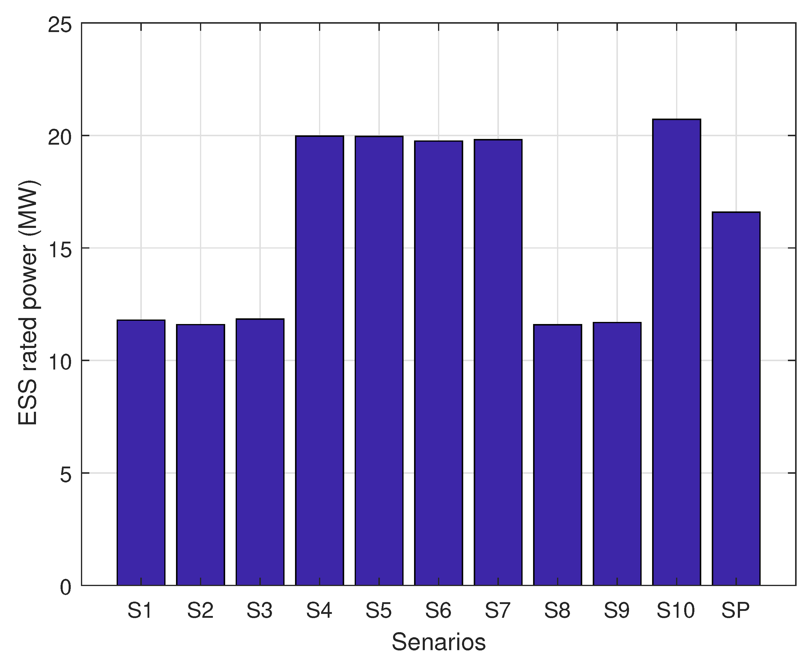
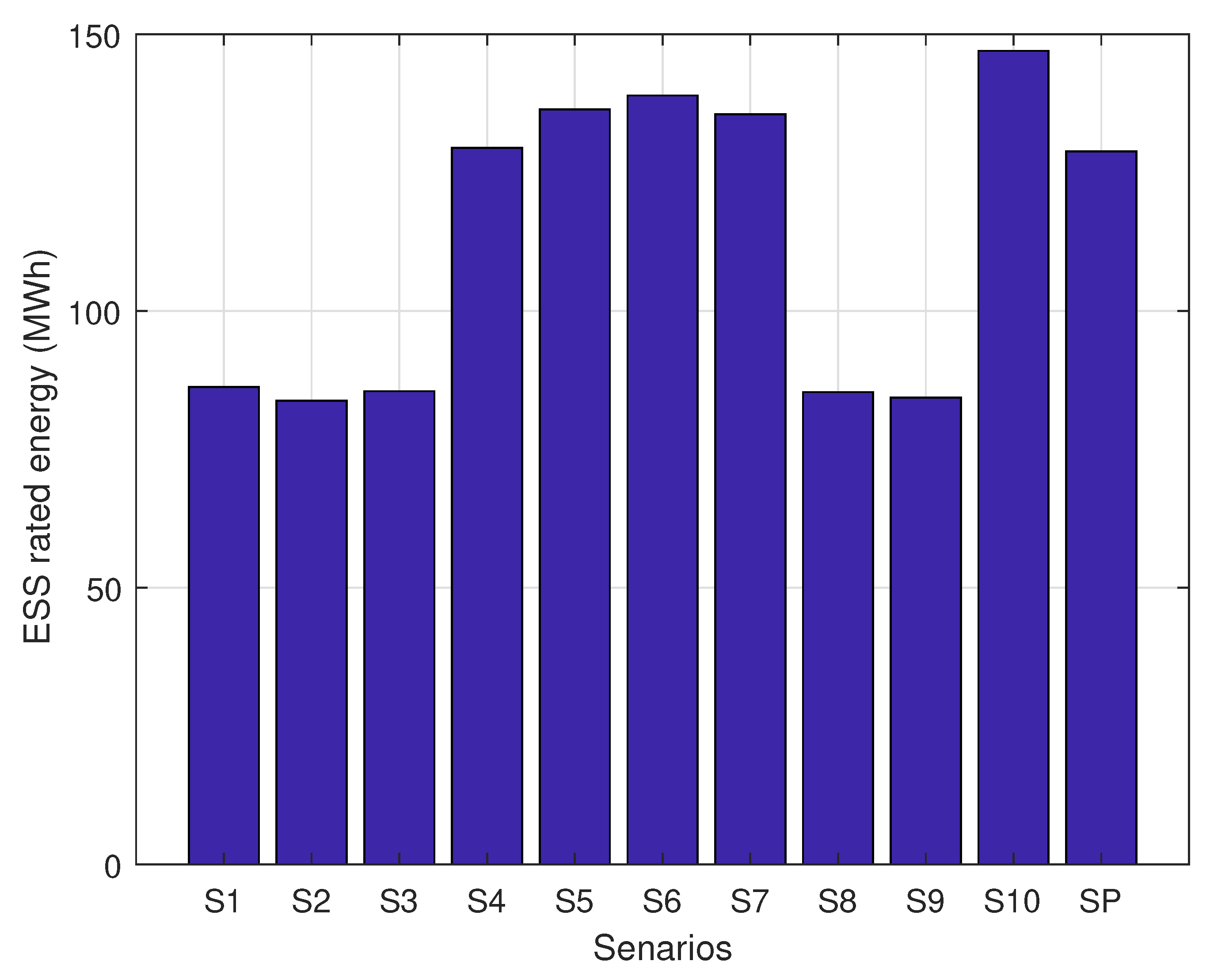
To prove that the stochastic programming method solution is reasonably optimal, using the mixed-integer linear programming method, the ten scenarios, previously assumed to be actual data for ten different years, have been solved separately. The outcomes are shown in

Table 6. Results of all scenarios solved separately.

Scenario	Total Cost ($)	${\mathit{P}}_{\mathit{S}}^{\mathit{R}}$ (MW)	${\mathit{E}}_{\mathit{S}}^{\mathit{R}}$ (MWh)
S1	14,634,417.23	11.79	86.23
S2	14,652,256.34	11.59	83.76
S3	14,648,323.41	11.84	85.50
S4	14,399,562.33	19.97	129.43
S5	14,393,281.42	19.96	136.42
S6	14,380,884.59	19.75	138.91
S7	14,414,730.03	19.81	135.50
S8	14,691,929.52	11.58	85.34
S9	14,645,579.66	11.69	84.33
S10	14,429,380.07	20.71	146.98
SP	14,392,584.15	16.59	128.84

and are contrasted in

Table 7. Comparison of results of all scenarios with SP solution.

Scenario	% Total Cost	%${\mathit{P}}_{\mathit{S}}^{\mathit{R}}$	%${\mathit{E}}_{\mathit{S}}^{\mathit{R}}$
S1	−1.6803%	28.9064%	33.0716%
S2	−1.8042%	30.1084%	34.9909%
S3	−1.7769%	28.5996%	33.6401%
S4	−0.0485%	−20.4079%	−0.4634%
S5	−0.0048%	−20.3461%	−5.8826%
S6	0.0813%	−19.0800%	−7.8221%
S7	−0.1539%	−19.4598%	−5.1736%
S8	−2.0799%	30.1612%	33.7609%
S9	−1.7578%	29.5432%	34.5429%
S10	−0.2557%	−24.8912%	−14.0825%

with the solution of the stochastic programming technique. The probabilistic optimization process solution is the second-best solution after Scenario 6 solution. So, this demonstrates that the probabilistic method provides a sensible alternative in comparison with the ten scenarios’ determinist method. A reasonable solution here means a better solution which leads to the minimum cost. These model and technique will help a microgrid developer to make a better economic decision on ESS sizing. The stochastic programming technique is used when there is more than one scenario and better outcomes are obtained as shown in Tabels Table 6 and Table 7. While in stochastic programming solution the investment cost of the storage system is greater than in other situations, the total cost is still smaller. The goal is to minimize the total cost, not the cost of investment. Scenario 6’s solution is smaller than the stochastic programming solution, but instead of all situations it represents only one scenario. The results of deterministic and probabilistic optimization problems are illustrated also in Figure 16, Figure 17 and Figure 18 to be read and compared easily.

In both cases, reliability indices were calculated to illustrate how reliability indices improve after the microgrid integration of the optimally sized ESS. In both cases, the reliability indices are shown in

Table 8. Comparison between the two cases.

Term	Case-1	Case-2	%Change
Net Cost ($)	7.108261 × 10${}^6$	7.096726 × 10${}^6$	−0.1625%
ASAI	9.9995 × 10${}^{-1}$	10.0000 × 10${}^{-1}$	0.0047%
ASUI	5.2200 × 10${}^{-5}$	4.7454 × 10${}^{-6}$	−90.9091%
SAIFI	1.7228 × 10${}^{-10}$	5.7054 × 10${}^{-13}$	−99.6688%
SAIDI	1.7228 × 10${}^{-8}$	6.5613 × 10${}^{-11}$	−99.6191%
CAIDI	1.0000 × 10${}^2$	1.1500 × 10${}^2$	15.0000%

. It also demonstrates the energy cost of manufacturing in both instances. Following integration of the ESS, the cost of manufacturing reduces as shown in this table. In addition, the microgrid’s accessibility is improving. The load point-related reliability indices are enhancing noticeable distinctions. It is also discovered that SAIFI and SAIDI are within the suggested boundaries.

One of the goals of incorporating the optimally sized ESS with the microgrid is to improve the reliability of the microgrid and this goal has been accomplished. After integration of the ESS, the microgrid integrated with the ESS works with greater accessibility and reduced cost. In addition, as shown in Figure 12, although the system sells more electricity to the main grid to reduce net costs and compensate for high production costs, and as shown in Figure 13, although the system purchases more electricity from the main grid, the net cost in Case 1 is still greater than Case 2. In the second case, the net cost also includes the ESS investment cost. Naturally, in both cases the net cost is the minimum possible cost to supply electrical energy to the demand. While this comparison is only for the first twenty-four hours, the whole horizon can be generalized. This clarifies the important economic advantages of microgrid integration of the ESS. To find the optimal size of an ESS to be integrated with any microgrid, other optimization techniques could be used. In addition, other methods could be used to enhance a microgrid’s reliability in particular.

Moreover, using the other approach illustrated in Algorithm 2, the optimal size of an ESS has been calculated as well. As mentioned previously, this method might give more economic results. The investment cost in this method is less than the investment cost calculated in the first approach. The rated power of the optimally sized ESS in this technique is 15.87 MW and the rated energy is 111.24 MWh. The investment cost of this ESS is about $52,416. This cost is less than the investment cost in the first approach by 10.48%.

6. Conclusions

This paper has presented a methodology to enhance the reliability of a microgrid through integrating it with an optimally sized ESS. The optimal size of an ESS has been found under wind uncertainties and a probabilistic optimization method, stochastic programming, has been used for this purpose. Integrating a microgrid with an optimally sized ESS enhances its reliability by increasing the energy availability and reducing the costs. For a customer, integrating an optimally sized ESS is important because it decreases the number of interruptions and reduces the interruption durations. Other techniques such as upgrading the generators and system components can be used to improve the reliability indicators for a customer. However, integrating the ESS is more reliable economically and this shows the economical feasibility of the system. While the ESS will cost in terms of investment cost, the total cost is still less and the system is more reliable and economical. This proposed methodology can be used in finding the optimal size of an ESS in systems integrated with renewable energy sources, such as wind turbines and solar cells because uncertainty matters in these systems and some parameters such as wind speed cannot be predicted accurately. As the integration of renewable energy sources increases and the importance of them gets higher, the necessity of integrating ESSs gets higher as well. The proposed methodology is significant to find the required size of an ESS to be integrated with those systems.

References

1. Gao, D.W. Energy Storage for Sustainable Microgrid; Academic Press: Cambridge, MA, USA, 2015. [Google Scholar]
2. Abdulgalil, M.A.; Amin, A.M.; Khalid, M.; AlMuhaini, M. Optimal Sizing, Allocation, Dispatch and Power Flow of Energy Storage Systems Integrated with Distributed Generation Units and a Wind Farm. In Proceedings of the IEEE PES Asia-Pacific Power and Energy Engineering Conference (APPEEC), Kota Kinabalu, Malaysia, 7–10 October 2018; pp. 680–684. [Google Scholar]
3. Abdulgalil, M.; Khalid, M. Enhancing the Reliability of a Microgrid Through Optimal Size of Battery Energy Storage System. IET Gener. Trans. Distrib. 2019, 13, 1499–1508. [Google Scholar] [CrossRef]
4. Bahramirad, S.; Camm, E. Practical modeling of Smart Grid SMS™ storage management system in a microgrid. In Proceedings of the Transmission and Distribution Conference and Exposition (T&D), Orlando, FL, USA, 7–10 May 2012; pp. 1–7. [Google Scholar]
5. Kienle, F.; de Schryver, C. 100% Green Computing At The Wrong Location? IEC—IEEE CHALLENGE: Geneva, Switzerland, 2012. [Google Scholar]
6. Adefarati, T.; Bansal, R. Integration of renewable distributed generators into the distribution system: A review. IET Renew. Power Gener. 2016, 10, 873–884. [Google Scholar] [CrossRef]
7. Bahramirad, S.; Reder, W.; Khodaei, A. Reliability-constrained optimal sizing of energy storage system in a microgrid. IEEE Trans. Smart Grid 2012, 3, 2056–2062. [Google Scholar] [CrossRef]
8. Chen, S.; Gooi, H.B.; Wang, M. Sizing of energy storage for microgrids. IEEE Trans. Smart Grid 2012, 3, 142–151. [Google Scholar] [CrossRef]
9. Singh, S.; Singh, M.; Kaushik, S.C. Optimal power scheduling of renewable energy systems in microgrids using distributed energy storage system. IET Renew. Power Gener. 2016, 10, 1328–1339. [Google Scholar] [CrossRef]
10. Abdulgalil, M.A.; Khalid, M.; Alismail, F. Optimizing a Distributed Wind-Storage System Under Critical Uncertainties Using Benders Decomposition. IEEE Access 2019. [Google Scholar] [CrossRef]
11. Chen, C.; Duan, S.; Cai, T.; Liu, B.; Hu, G. Smart energy management system for optimal microgrid economic operation. IET Renew. Power Gener. 2011, 5, 258–267. [Google Scholar] [CrossRef]
12. Abdulgalil, M.A.; Elsayed, A.H.; Khalid, M.; ElAmin, I.M. Optimal Dispatch of Distributed Generation Units, Wind Farms and Energy Storage Systems. In Proceedings of the IEEE PES Asia-Pacific Power and Energy Engineering Conference (APPEEC), Sabah, Malaysia, 7–10 October 2018; pp. 668–673. [Google Scholar]
13. Zhou, L.; Zhang, Y.; Lin, X.; Li, C.; Cai, Z.; Yang, P. Optimal sizing of PV and BESS for a smart household considering different price mechanisms. IEEE Access 2018, 6, 41050–41059. [Google Scholar] [CrossRef]
14. Bahramirad, S.; Daneshi, H. Optimal sizing of smart grid storage management system in a microgrid. In Proceedings of the IEEE PES Innovative Smart Grid Technologies (ISGT), Tianjin, China, 21–24 May 2012; pp. 1–7. [Google Scholar]
15. Akram, U.; Khalid, M.; Shafiq, S. An improved optimal sizing methodology for future autonomous residential smart power systems. IEEE Access 2018, 6, 5986–6000. [Google Scholar] [CrossRef]
16. Gupta, P.P.; Jain, P.; Sharma, S.; Bhakar, R. Reliability-Security Constrained Unit Commitment based on benders decomposition and Mixed Integer Non-Linear Programming. In Proceedings of the International Conference on Computer, Communications and Electronics (Comptelix), Jaipur, India, 1–2 July 2017; pp. 328–333. [Google Scholar]
17. Nguyen, T.A.; Crow, M.L.; Elmore, A.C. Optimal sizing of a vanadium redox battery system for microgrid systems. IEEE Trans. Sustain. Energy 2015, 6, 729–737. [Google Scholar] [CrossRef]
18. Abdulgalil, M.A.; Khater, M.N.; Khalid, M.; Alisamail, F. Sizing of energy storage systems to enhance microgrid reliability. In Proceedings of the IEEE International Conference on Industrial Technology (ICIT), Lyon, France, 20–22 February 2018; pp. 1302–1307. [Google Scholar]
19. Kerdphol, T.; Qudaih, Y.; Mitani, Y. Battery energy storage system size optimization in microgrid using particle swarm optimization. In Proceedings of the IEEE PES Innovative Smart Grid Technologies Conference Europe (ISGT-Europe), Istanbul, Turkey, 12–15 October 2014; pp. 1–6. [Google Scholar]
20. Huang, Y.; Pardalos, P.M.; Zheng, Q.P. Electrical Power Unit Commitment: Deterministic and Two-Stage Stochastic Programming Models and Algorithms; Springer: Berlin, Germany, 2017. [Google Scholar]
21. Xiong, P.; Jirutitijaroen, P.; Singh, C. A distributionally robust optimization model for unit commitment considering uncertain wind power generation. IEEE Trans. Power Syst. 2017, 32, 39–49. [Google Scholar] [CrossRef]
22. Mbungu, N.T.; Naidoo, R.; Bansal, R.C.; Bipath, M. Optimisation of grid connected hybrid photovoltaic– wind–battery system using model predictive control design. IET Renew. Power Gener. 2017, 11, 1760–1768. [Google Scholar] [CrossRef]
23. Zhang, L.; Hu, X.; Wang, Z.; Sun, F.; Deng, J.; Dorrell, D.G. Multiobjective Optimal Sizing of Hybrid Energy Storage System for Electric Vehicles. IEEE Trans. Veh. Technol. 2018, 67, 1027–1035. [Google Scholar] [CrossRef]
24. Akram, U.; Khalid, M.; Shafiq, S. An innovative hybrid wind-solar and battery-supercapacitor microgrid system—Development and optimization. IEEE Access 2017, 5, 25897–25912. [Google Scholar] [CrossRef]
25. Nikmehr, N.; Najafi-Ravadanegh, S. Optimal operation of distributed generations in micro-grids under uncertainties in load and renewable power generation using heuristic algorithm. IET Renew. Power Gener. 2015, 9, 982–990. [Google Scholar] [CrossRef]
26. Soroudi, A. Power System Optimization Modeling in GAMS; Springer: Cham, Switzerland, 2017. [Google Scholar]
27. Gee, A.M.; Robinson, F.; Yuan, W. A Superconducting Magnetic Energy Storage-Emulator/Battery Supported Dynamic Voltage Restorer. IEEE Trans. Energy Convers. 2017, 32, 55–64. [Google Scholar] [CrossRef]
28. Krupke, C.; Wang, J.; Clarke, J.; Luo, X. Modeling and Experimental Study of a Wind Turbine System in Hybrid Connection With Compressed Air Energy Storage. IEEE Trans. Energy Convers. 2017, 32, 137–145. [Google Scholar] [CrossRef]
29. Chang, X.; Li, Y.; Li, X.; Chen, X. An Active Damping Method Based on a Supercapacitor Energy Storage System to Overcome the Destabilizing Effect of Instantaneous Constant Power Loads in DC Microgrids. IEEE Trans. Energy Convers. 2017, 32, 36–47. [Google Scholar] [CrossRef]
30. Steffen, B. Prospects for pumped-hydro storage in Germany. Energy Policy 2012, 45, 420–429. [Google Scholar] [CrossRef] [Green Version]
31. Lujano-Rojas, J.M.; Dufo-López, R.; Bernal-Agustín, J.L.; Catalão, J.P. Optimizing Daily Operation of Battery Energy Storage Systems Under Real-Time Pricing Schemes. IEEE Trans. Smart Grid 2017, 8, 316–330. [Google Scholar] [CrossRef]
32. Daoud, M.I.; Massoud, A.M.; Abdel-Khalik, A.S.; Elserougi, A.; Ahmed, S. A flywheel energy storage system for fault ride through support of grid-connected VSC HVDC-based offshore wind farms. IEEE Trans. Power Syst. 2016, 31, 1671–1680. [Google Scholar] [CrossRef]
33. Park, C.; Sedundo, R.; Knazkins, V.; Korbakorba, P. Feasibility analysis of the power-to-gas concept in the future Swiss power system. In Proceedings of the CIRED Workshop 2016, Helsinki, Finland, 14–15 June 2016; IET: Stevenage, UK, 2016. [Google Scholar]
34. Beardsall, J.C.; Gould, C.A.; Al-Tai, M. Energy storage systems: A review of the technology and its application in power systems. In Proceedings of the 50th International Universities Power Engineering Conference (UPEC), Stoke-on-Trent, UK, 1–4 September 2015; pp. 1–6. [Google Scholar]
35. Pulendran, S.; Tate, J.E. Energy storage system control for prevention of transient under-frequency load shedding. IEEE Trans. Smart Grid 2017, 8, 927–936. [Google Scholar]
36. Borges, C.L.; Falcao, D.M. Optimal distributed generation allocation for reliability, losses, and voltage improvement. Int. J. Electr. Power Energy Syst. 2006, 28, 413–420. [Google Scholar] [CrossRef]
37. Maghouli, P.; Soroudi, A.; Keane, A. Robust computational framework for mid-term techno-economical assessment of energy storage. IET Gener. Trans. Distrib. 2016, 10, 822–831. [Google Scholar] [CrossRef]
38. Sun, S.; Liang, B.; Dong, M.; Taylor, J.A. Phase Balancing Using Energy Storage in Power Grids Under Uncertainty. IEEE Trans. Power Syst. 2016, 31, 3891–3903. [Google Scholar] [CrossRef]
39. Vargas, L.S.; Bustos-Turu, G.; Larraín, F. Wind power curtailment and energy storage in transmission congestion management considering power plants ramp rates. IEEE Trans. Power Syst. 2015, 30, 2498–2506. [Google Scholar] [CrossRef]
40. Soroudi, A.; Siano, P.; Keane, A. Optimal DR and ESS scheduling for distribution losses payments minimization under electricity price uncertainty. IEEE Trans. Smart Grid 2016, 7, 261–272. [Google Scholar] [CrossRef]
41. Khalid, M.; Akram, U.; Shafiq, S. Optimal Planning of Multiple Distributed Generating Units and Storage in Active Distribution Networks. IEEE Access 2018, 6, 55234–55244. [Google Scholar] [CrossRef]
42. Li, Y.; Yang, Z.; Li, G.; Zhao, D.; Tian, W. Optimal scheduling of an isolated microgrid with battery storage considering load and renewable generation uncertainties. IEEE Trans. Ind. Electron. 2019, 66, 1565–1575. [Google Scholar] [CrossRef]
43. Li, Y.; Yang, Z.; Li, G.; Mu, Y.; Zhao, D.; Chen, C.; Shen, B. Optimal scheduling of isolated microgrid with an electric vehicle battery swapping station in multi-stakeholder scenarios: A bi-level programming approach via real-time pricing. Appl. Energy 2018, 232, 54–68. [Google Scholar] [CrossRef] [Green Version]
44. Li, Y.; Feng, B.; Li, G.; Qi, J.; Zhao, D.; Mu, Y. Optimal distributed generation planning in active distribution networks considering integration of energy storage. Appl. Energy 2018, 210, 1073–1081. [Google Scholar] [CrossRef] [Green Version]
45. Jamali, A.; Nor, N.; Ibrahim, T. Energy storage systems and their sizing techniques in power system—A review. In Proceedings of the IEEE Conference on Energy Conversion (CENCON), Johor Bahru, Malaysia, 19–20 October 2015; pp. 215–220. [Google Scholar]
46. Milligan, M.; Donohoo, P.; Lew, D.; Ela, E.; Kirby, B.; Holttinen, H.; Lannoye, E.; Flynn, D.; O’Malley, M.; Miller, N.; et al. Operating Reserves and Wind Power Integration: An International Comparison; Technical Report; National Renewable Energy Lab.(NREL): Golden, CO, USA, 2010.
47. Holttinen, H.; Milligan, M.; Ela, E.; Menemenlis, N.; Dobschinski, J.; Rawn, B.; Bessa, R.J.; Flynn, D.; Gomez-Lazaro, E.; Detlefsen, N.K. Methodologies to determine operating reserves due to increased wind power. IEEE Trans. Sustain. Energy 2012, 3, 713–723. [Google Scholar] [CrossRef]
48. Barton, J.P.; Infield, D.G. A probabilistic method for calculating the usefulness of a store with finite energy capacity for smoothing electricity generation from wind and solar power. J. Power Sour. 2006, 162, 943–948. [Google Scholar] [CrossRef] [Green Version]
49. Tofighi, A.; Kalantar, M. Power management of PV/battery hybrid power source via passivity-based control. Renew. Energy 2011, 36, 2440–2450. [Google Scholar] [CrossRef]
50. Díaz-González, F.; Sumper, A.; Gomis-Bellmunt, O.; Villafáfila-Robles, R. A review of energy storage technologies for wind power applications. Renew. Sustain. Energy Rev. 2012, 16, 2154–2171. [Google Scholar] [CrossRef]
51. Tan, X.; Li, Q.; Wang, H. Advances and trends of energy storage technology in Microgrid. Int. J. Electr. Power Energy Syst. 2013, 44, 179–191. [Google Scholar] [CrossRef]
52. Yamin, H.; Shahidehpour, S. Unit commitment using a hybrid model between Lagrangian relaxation and genetic algorithm in competitive electricity markets. Electr. Power Syst. Res. 2004, 68, 83–92. [Google Scholar] [CrossRef]
53. Kempton, W.; Tomić, J. Vehicle-to-grid power implementation: From stabilizing the grid to supporting large-scale renewable energy. J. Power Sources 2005, 144, 280–294. [Google Scholar] [CrossRef]
54. Masaud, T.M.; Lee, K.; Sen, P. An overview of energy storage technologies in electric power systems: What is the future? In Proceedings of the North American Power Symposium 2010, Arlington, TX, USA, 26–28 September 2010; pp. 1–6. [Google Scholar]
55. Rodrigues, E.; Godina, R.; Santos, S.; Bizuayehu, A.; Contreras, J.; Catalão, J. Energy storage systems supporting increased penetration of renewables in islanded systems. Energy 2014, 75, 265–280. [Google Scholar] [CrossRef]
56. Kousksou, T.; Bruel, P.; Jamil, A.; El Rhafiki, T.; Zeraouli, Y. Energy storage: Applications and challenges. Sol. Energy Mater. Sol. Cells 2014, 120, 59–80. [Google Scholar] [CrossRef]
57. Bhatnagar, N.; Venkatesh, B. Energy storage and power systems. In Proceedings of the 25th IEEE Canadian Conference on Electrical and Computer Engineering (CCECE), Montreal, QC, Canada, 29 April–2 May 2012; pp. 1–4. [Google Scholar]
58. Bhuiyan, F.A.; Yazdani, A. Energy storage technologies for grid-connected and off-grid power system applications. In Proceedings of the IEEE Electrical Power and Energy Conference, London, ON, Canada, 10–12 October 2012; pp. 303–310. [Google Scholar]
59. Vazquez, S.; Lukic, S.M.; Galvan, E.; Franquelo, L.G.; Carrasco, J.M. Energy storage systems for transport and grid applications. IEEE Trans. Ind. Electr. 2010, 57, 3881–3895. [Google Scholar] [CrossRef]
60. Saez-de Ibarra, A.; Milo, A.; Gaztañaga, H.; Etxeberria-Otadui, I.; Rodríguez, P.; Bacha, S.; Debusschere, V. Analysis and comparison of battery energy storage technologies for grid applications. In Proceedings of the IEEE Grenoble Conference, Grenoble, France, 16–20 June 2013; pp. 1–6. [Google Scholar]
61. Romlie, M.F.; Klumpner, C.; Rashed, M.; Odavic, M.; Asher, G. Analysis of stability aspects of a large constant power load in a local grid. In Proceedings of the 15th European Conference on Power Electronics and Applications (EPE), Lille, France, 2–6 September 2013; pp. 1–11. [Google Scholar]
62. Divya, K.; Østergaard, J. Battery energy storage technology for power systems—An overview. Electr. Power Syst. Res. 2009, 79, 511–520. [Google Scholar] [CrossRef]
63. Sharma, A.; Tyagi, V.V.; Chen, C.; Buddhi, D. Review on thermal energy storage with phase change materials and applications. Renew. Sustain. Energy Rev. 2009, 13, 318–345. [Google Scholar] [CrossRef]
64. Burnett, D.; Barbour, E.; Harrison, G.P. The UK solar energy resource and the impact of climate change. Renew. Energy 2014, 71, 333–343. [Google Scholar] [CrossRef] [Green Version]
65. Gaetani, M.; Huld, T.; Vignati, E.; Monforti-Ferrario, F.; Dosio, A.; Raes, F. The near future availability of photovoltaic energy in Europe and Africa in climate-aerosol modeling experiments. Renew. Sustain. Energy Rev. 2014, 38, 706–716. [Google Scholar] [CrossRef]
66. Akhil, A.A.; Huff, G.; Currier, A.B.; Kaun, B.C.; Rastler, D.M.; Chen, S.B.; Cotter, A.L.; Bradshaw, D.T.; Gauntlett, W.D. DOE/EPRI 2013 Electricity Storage Handbook in Collaboration with NRECA; Sandia National Laboratories Albuquerque: Livermore, CA, USA, 2013.
67. Chen, Y.; Zheng, Y.; Luo, F.; Wen, J.; Xu, Z. Reliability evaluation of distribution systems with mobile energy storage systems. IET Renew. Power Gener. 2016, 10, 1562–1569. [Google Scholar] [CrossRef]
68. Electricity Storage Technologies Can Be Used for Energy Management and Power Quality. 2011. Available online: https://www.eia.gov/todayinenergy/detail.php?id=4310 (accessed on 15 January 2019).
69. Higle, J.L. Stochastic programming: Optimization when uncertainty matters. Tutor. Oper. Res. 2005, 30–53. [Google Scholar] [CrossRef]
70. Jacob, A.S.; Banerjee, R.; Ghosh, P.C. Sizing of hybrid energy storage system for a PV based microgrid through design space approach. Appl. Energy 2018, 212, 640–653. [Google Scholar] [CrossRef]
71. Kalvelagen, E. Benders Decomposition with GAMS; Amsterdam Optimization Modeling Group: Washington, DC, USA, 2002. [Google Scholar]
72. Abdulgalil, M.A.; Alharbi, H.S.; Khalid, M.; Almuhaini, M.M. Reliability Assessment of Microgrids with Multiple Distributed Generations and Hybrid Energy Storage. In Proceedings of the IEEE 27th International Symposium on Industrial Electronics (ISIE), Cairns, Australia, 12–15 June 2018; pp. 868–873. [Google Scholar]
73. Castillo, E.; Conejo, A.J.; Pedregal, P.; Garcia, R.; Alguacil, N. Building and Solving Mathematical Programming Models in Engineering and Science; John Wiley & Sons: Haboken, NJ, USA, 2011; Volume 62. [Google Scholar]
74. Chattopadhyay, D. Application of general algebraic modeling system to power system optimization. IEEE Trans. Power Syst. 1999, 14, 15–22. [Google Scholar] [CrossRef]
75. Akram, U.; Khalid, M. A coordinated frequency regulation framework based on hybrid battery-ultracapacitor energy storage technologies. IEEE Access 2018, 6, 7310–7320. [Google Scholar] [CrossRef]
76. Simopoulos, D.; Giannakopoulos, Y.; Kavatza, S.; Vournas, C. Effect of emission constraints on short-term unit commitment. In Proceedings of the MELECON 2006—2006 IEEE Mediterranean Electrotechnical Conference, Malaga, Spain, 16–19 May 2006; pp. 973–977. [Google Scholar]
77. Wind Turbine Power Curve Definitions. Available online: http://www.wind-power-program.com/popups/powercurve.htm (accessed on 15 January 2019).
78. Zou, J.; Peng, C.; Shi, J.; Xin, X.; Zhang, Z. State-of-charge optimising control approach of battery energy storage system for wind farm. IET Renew. Power Gener. 2015, 9, 647–652. [Google Scholar] [CrossRef]
79. Force, R.T. The IEEE reliability test system-1996. IEEE Trans. Power Syst. 1999, 14, 1010–1020. [Google Scholar]
80. Rehman, S.; Halawani, T.; Husain, T. Weibull parameters for wind speed distribution in Saudi Arabia. Sol. Energy 1994, 53, 473–479. [Google Scholar] [CrossRef]
81. GAMS—Cutting Edge Modeling. Available online: https://www.gams.com/ (accessed on 15 January 2019).
82. NEOS Server for Optimization. Available online: https://neos-server.org/neos/ (accessed on 15 January 2019).
Figure 1. Schematic of centralized and distributed systems [5].
Energies 12 02412 g001
Figure 2. Schematic of inputs and outputs of Smart Energy Management System (SEMS).
Energies 12 02412 g002
Figure 3. Cost vs. energy storage system (ESS) size.
Energies 12 02412 g003
Figure 4. The flowchart of the proposed algorithm.
Energies 12 02412 g004
Figure 5. Electricity storage technologies [68].
Energies 12 02412 g005
Figure 6. Wind power vs. wind speed [77].
Energies 12 02412 g006
Figure 7. Parallel components in a microgrid.
Energies 12 02412 g007
Figure 8. Wind frequency histogram and Weibull distribution for all wind speeds in Dhahran.
Energies 12 02412 g008
Figure 9. Load curve and load duration curve.
Energies 12 02412 g009
Figure 10. Average daily wind speeds of the ten scenarios.
Energies 12 02412 g010
Figure 11. Hourly wind speeds during the first twenty-four hours of the ten scenarios.
Energies 12 02412 g011
Figure 12. Economic dispatch without ESS.
Energies 12 02412 g012
Figure 13. Economic dispatch with ESS.
Energies 12 02412 g013
Figure 14. ESS power and exchanged power with negative values.
Energies 12 02412 g014
Figure 15. Stored energy in ESS.
Energies 12 02412 g015
Figure 16. Total cost of all scenarios.
Energies 12 02412 g016
Figure 17. ESS rated power of all scenarios.
Energies 12 02412 g017
Figure 18. ESS rated energy of all scenarios.
Energies 12 02412 g018