“Dust in the Wind...”, Deep Learning Application to Wind Energy Time Series Forecasting

Abstract

To balance electricity production and demand, it is required to use different prediction techniques extensively. Renewable energy, due to its intermittency, increases the complexity and uncertainty of forecasting, and the resulting accuracy impacts all the different players acting around the electricity systems around the world like generators, distributors, retailers, or consumers. Wind forecasting can be done under two major approaches, using meteorological numerical prediction models or based on pure time series input. Deep learning is appearing as a new method that can be used for wind energy prediction. This work develops several deep learning architectures and shows their performance when applied to wind time series. The models have been tested with the most extensive wind dataset available, the National Renewable Laboratory Wind Toolkit, a dataset with 126,692 wind points in North America. The architectures designed are based on different approaches, Multi-Layer Perceptron Networks (MLP), Convolutional Networks (CNN), and Recurrent Networks (RNN). These deep learning architectures have been tested to obtain predictions in a 12-h ahead horizon, and the accuracy is measured with the coefficient of determination, the R² method. The application of the models to wind sites evenly distributed in the North America geography allows us to infer several conclusions on the relationships between methods, terrain, and forecasting complexity. The results show differences between the models and confirm the superior capabilities on the use of deep learning techniques for wind speed forecasting from wind time series data.

1. Introduction

The development of clean electricity is one pivotal area for the transition to a de-carbonized world, and for this reason, the electricity systems are under a process of transformation from a heavily-centralized network, based on large uranium, coal, gas or gas-oil generation plants, to a new decentralized model with small wind or solar units that require high coordination, accomplished by the intensive use of computer algorithms [1]. The quintessential renewable energy source has always been the hydro-based generation, found in many forms, from very large dams that produce hundreds of MW, to small units that output a few KW of electricity from running water sources. Hydro energy is inexpensive and secure, and by adding different versions of pumped-storage technologies, dams can be transformed into electricity storage systems, helping to regulate the electricity systems around the world [2]. However, this energy depends on water, a resource not always available or scarce, and cannot be ramped up to cover the energy needs of the world, opening the door for other clean sources. Solar and wind show the fastest growth around the globe. Both technologies share the intermittency issues inherent to renewables; hence, forecasting becomes a critical process to integrate all these new sources while keeping the grid stable. There are different studies regarding the importance of forecasting in the grid integration like [3] or [4], which show, with modeling performed at the European level, how relevant the forecasting processes are, for short-, mid- and long-term, to assure grid stability [5].

Wind energy prediction can be classified into two major approaches depending on the origin of the input, meteorological or time series. The first class, also known as physical forecasting [6], is based on the use of Numerical Weather Prediction models (NWP) as an input, while the time series prediction is based only on using time-stamped past observations. In this work, the focus is on the second approach, as the objective of this research is to determine how some deep learning architectures can learn wind patterns from past observations.

Wind speed time series, from the statistics standpoint, have some characteristics that define their prediction as a complex problem (for an analysis of wind energy prediction, see [7]). The wind series show non-linearity and, most of the time, also non-stationarity (see Section 2.1), which makes the use of linear modeling methods like Auto-Regressive methods (AR), Moving Average Methods (MA), or combinations of both (ARIMA) inaccurate for commercial use, unless they are complemented with additional tools to cope with the non-linearity like Nonlinear Auto-Regressive Exogenous models (NARX) [8], or by combining methods with decomposition of the wind wave, like using Fourier or wavelet transformations [9]. Another approach consists of using combinations of methods or ensembles [10].

The introduction of machine learning algorithms in the wind prediction field has occurred in parallel with the development of software tools to use these models on a large scale. These new tools have allowed the design of approaches with good accuracy results applied to wind time series. Machine learning in wind approaches has been documented using different conceptual paths like Bayesian approaches in [11,12,13], k-Nearest Neighbor (k-NN) algorithms in [14] or [15], and Support Vector Machines (SVM) in [16,17] (see a complete literary review in [18]).

Neural network methods started slowly due to some concerns about their applicability to time series, but in the last few years, they have shown traction with some Multi-Layer Perceptron models (MLP) [19,20,21]. More recently, deep learning architectures are showing their potential in wind time series forecasting [22], with applications of recurrent neural networks [23,24,25] or convolutional networks in [26,27] (for a complete review of deep learning architectures applied to wind energy forecasting, see [28]).

The objective of wind energy forecasting is to predict the energy generated by a wind turbine or by a wind farm (set of turbines) in a future time horizon. The conversion of the wind energy into electricity is based on the air kinetic conversion principle (see Equation (1)).

$$E=\frac{1}{2}\rho At{v}^3$$

(1)

where $\rho$ is air density, A is blade swept area, v is wind speed, and t is time. In this formula, it can be observed that the major input contributor is wind speed ($v^3$). In practice, the conversion from wind speed to energy is not as direct as this formula implies, as there are many factors acting in the transformation from speed to energy (wind direction, turbine maintenance, specifics of the generation engine, etc.), as this conversion is obtained by applying a turbine-specific power curve function, which is non-linear and has some uncertainty ([29,30]).

Predicting energy output of a turbine is a two step process, the first one is to forecast the wind speed, while the second one consists of applying the power curve to this value. As the power curve has a cut-in (wind speed point where the turbine starts generating), a cut-out (wind speed point where the turbine stops generating as it is too fast), and the curve shape has a steep slope, the error propagation between the wind speed and energy is non-trivial, as this slope and these cut points can decrease or amplify the error intensity. In addition to these issues, the turbine has mechanical components that can impact generation if they lack in maintenance, have wear of parts, and small damages. Altogether, it is clear that the theoretical power curve needs to be adjusted to the technical situation of the turbine [31].

This work focuses on the wind speed forecasting process by developing several deep learning models (see

Table 1. Models developed in the experiments with short description and abbreviation used in article.

Model	Description	Abbr Used
Multi-Layer Perceptron	MLP sequence to sequence	MLP
Multi-Layer Perceptron	MLP with Direct regression	MLP Dir
Convolutional Network	CNN sequence to sequence	CNN
Recurrent Neural Network	RNN Encoder Decoder	RNN ED
Recurrent Neural Network	RNN seq2seq	RNN
k-NN	k-NN neighbors	k-NN
Persistence	Traditional persistence	Pers

) to predict wind speed at a 12-h ahead horizon, a time window that can be considered mid-term in the wind forecasting field. The experiments were executed on the NREL dataset (with 126,692 wind sites), and the cumulative values of accuracy were measured with the coefficient of determination or $R^2$.

The main contribution consists not only of the definition of novel deep learning architectures, but in the application of these models extensively on the largest publicly-available wind dataset. The NREL data offer wind sites distributed evenly in North America, and this allows going far beyond the traditional application of some methods to a single wind farm or to a small number of sites. The variability of the sites’ topology allows us to observe geographical relationships between sites and wind complexity and to draw inferences connecting the best method accuracy with site location.

The availability of computing power has been made possible by the collaboration with the Barcelona Super-computing Center (BSC) [32], which has provided their infrastructure (MinoTauro GPU cluster) to support the experiments.

As a summary, this work looks into the capabilities of deep learning in understanding past patterns of wind observations in order to predict future wind behavior. Wind is formed by a complex interaction of several natural phenomena and local features; the intricacy of its formation explains its prediction difficulty, and for this new set of algorithms to understand the subtlety of its patterns, they need to be able to learn from insignificant pieces of information that are not apparent, like meaningless dust specks in the wind, like the metaphorical “Dust in the Wind” in the well-known song from Kansas.

The organization of the paper is as follows: It starts with Section 2 with the introduction of the wind forecasting problem, then develops the time series approach plus the principles of deep learning for forecasting, closing with the description of the data used for experimentation. Section 3 analyzes the different methods used for data pre-processing, architecture design, and error measurement, including the analysis of the hyper-parameter setting process and the overall experimental setup. Section 4 compares and analyzes all the experimental results, and finally, Section 5 analyzes the overall work, developing conclusions and future lines of work.

2. Wind Time Series Forecasting

2.1. Wind Time Series Characteristics

Wind time series are based on multiple observations performed at a specific location or wind site (in wind generation, these data are usually generated by the turbine sensor devices). In this work, the time series contains five dimensions, which are wind speed, temperature, humidity, pressure, and direction, recorded every 5 min (see

Table 2. Variables in an NREL wind dataset time step.

Variable	Description
Time	Time stamp in UTC
Wind Speed	Wind speed measured in m/s at a 100-m height
Wind Direction	Wind direction at a 100-m height (0–360°)
Temperature	Temperature at 2 m  from the ground level in K
Barometric Pressure	Pressure at a 100-m height in Pa
Air Density	Air density at a 100-m height in kg/m${}^3$

).

Wind time series have two relevant characteristics, the first one being stationarity, which is a time series property found when the series has a mean or variance (or both) that does not change over time, and the second being linearity, observed in a time series when linear modeling can represent the co-variance structure of the series [33] (linear modeling like Auto-Regressive (AR) or Moving Average (MA) methods). As wind time series in most cases do not show stationarity or linearity, they must be modeled using non-linear approaches.

2.2. Multiple-Step-Ahead Forecasting

One challenging problem with time series forecasting is to obtain predictions in a horizon beyond the next time step, a problem that is defined as multiple-step-ahead forecasting.

Multiple-step-ahead forecasting can be interpreted as a multiple regression problem, where the past data are used to obtain multiple prediction steps in the future. There are several methods to approach this problem, which can be summarized into two [34]. The first one is the recursive approach where one model is trained to estimate the first step ahead, and then, the successive steps are computed recursively using each generated step as an input value. The main disadvantage of this method lays in the fact that the error of the prediction is propagated to successive predictions. Usually, this method does not yield the best results.

The second method is the direct forecasting, a strategy with two different approaches depending on how the predictions are obtained. The first one is to obtain a model for each step on the horizon that has to be predicted. This means that a different model is trained to minimize the error for each time step separately, a computationally-expensive approach. The second method consists of a model that generates multiple outputs by training the model to minimize the error for all the time steps in the horizon at the same time. This method is also known as the Multiple Input Multiple Output (MIMO) approach. A compromise between the two approaches is also possible by obtaining separate models that predict subsets of steps.

As the MIMO approach input is a sequence and the output is another sequence, in the deep learning field, it is commonly defined as sequence to sequence or seq2seq. For the sake of clarity in this article, the seq2seq nomenclature will be used, taking into account that it is understood as a synonym of MIMO.

2.3. Forecasting Time Series with Deep Learning

Given a time series $\mathbf{X}$ of n elements $\left[{\mathit{x}}_1,{\mathit{x}}_2,{\mathit{x}}_3,\cdots ,{\mathit{x}}_n\right]$, a prediction is obtained for H (horizon) steps ahead $\widehat{\mathbf{Y}}=\left[{\widehat{\mathit{y}}}_{n+1},{\widehat{\mathit{y}}}_{n+2},\cdots ,{\widehat{\mathit{y}}}_{n+H}\right]$. To train the DLarchitectures, a set of examples is generated $\mathbf{Z}=\left[{\mathit{z}}_1,{\mathit{z}}_2,\cdots ,{\mathit{z}}_k\right]$. The set of examples $\mathbf{Z}$ is formed by elements ${\mathit{z}}_i$ that contain sections of the wind series of length lag. To have better accuracy, the larger the set of examples $\mathbf{Z}$ is, the better. It is well known that deep learning architectures do not generalize well from a small number of examples, and they require large amounts of data for training [35].

The deep models are trained with the example set $\mathbf{Z}$ and then are able to perform predictions for horizon H steps with real input from the series. In this work, the predictions and measures of accuracy (see Section 3.3) are made on the test and validation datasets by analyzing the distance between the predicted $\widehat{\mathbf{Y}}$ values and the real observations $\left[{\mathit{x}}_{n+1},{\mathit{x}}_{n+2},{\mathit{x}}_{n+3},\cdots ,{\mathit{x}}_{n+H}\right]$ that are found in the dataset. For some comparisons in this work, the sum of the 12 step values is used as a single performance measure of the accuracy ${\sum }_i^{12}{R}_i^2$.

2.4. Data: The National Renewable Laboratory Wind Dataset

To forecast wind energy with deep learning, access to large amounts of observations is required. The data from wind turbines usually belong to the turbine owner company and, as it may have some commercial value, is locked and not available to the research community [36], making it almost impossible for researchers to access open and large datasets of wind data.

This explains why in the wind prediction field, there is not a standard wind/energy dataset available, constraining each researcher to use small available sets from different geographies and short periods. This situation is difficult to understand as the investment in wind parks is heavily subsidized with public funds in many countries.

Nevertheless, the National Renewable Energy Laboratory in the U.S. (NREL) has developed a large wind dataset and made it publicly available. This dataset offers production and meteorological data (wind speed, wind direction, temperature, pressure, humidity, and energy) synthesized from meteorological global models for over 129,962 sites evenly placed in the U.S. geography. This dataset has been created with meteorological data from weather research and using the forecasting (WRF) model Version 3.4.1 [37], down-sampled to a 2-km and 5-min resolution for the interval 2007–2013. Then, some additional features were added, like model terrain, roughness, and some soil properties from the U.S. Geological Survey GTOPO30 data. The modeled result was validated with real observations to reduce errors and prove the final quality of the dataset [38]. Each item in a wind site time series contains the information shown in Table 2.

This dataset is the largest public dataset on wind, and its main advantage consists of its size and the geographical site distribution across all the latitudes and longitudes of the U.S.

The original data were sampled at 5-min intervals. A design decision in the experimentation has been to down-sample the dataset to 1-h intervals by computing hourly means, as the experimental results were not impacted and the amount of data managed was reduced by a factor of 12, reducing the resource requirements of the overall experimental process. This down-sampling is also justified by the fact that in practical scenarios of wind production, an hourly forecast is a reasonable figure.

3. Methods

In this section, the components of the research work are described, being the data preprocessing process, the architectures, the accuracy measurement, and a discussion on the computing side of the work, plus a description on how the parameters of each model have been determined.

3.1. Data Preprocessing

To have easier access to the data, the NREL dataset was subjected to preprocessing in order to ease the learning convergence of the models and to obtain more informative results from the executions.

The wind dataset had 126,692 wind sites with five measures (see Table 2) and contained seven years of data. For this work, it was divided into 3 subsets, training, test, and validation. The training subset contained five years (2007–2011) of information and was composed of the five measures averaged hourly. One year (2012) was reserved for testing and used to adjust the parameters of the models during the training, and the final year (2013) was reserved for validation of the different approaches. The objective of the experiments was to obtain wind speed predictions (in a twelve-hour horizon); this goal makes the wind speed the primary variable in the datasets, while the other 4 dimensions (wind direction, temperature, barometric pressure, and air density) were added as auxiliary variables. All the subsets of data were subjected to a preprocessing, which consisted of z-standardization of the data. This normalization was made by adjusting the scale of the values to obtain a mean of zero and a variance (${\sigma }^2$) of one. This is a usual data transformation process used when the data are used for neural network training [35].

A special mention is required for wind direction, as it has a special treatment because the raw degree averages might induce errors; for this reason, the values were transformed from the original degree to their sine and cosine.

3.2. The Architecture Components

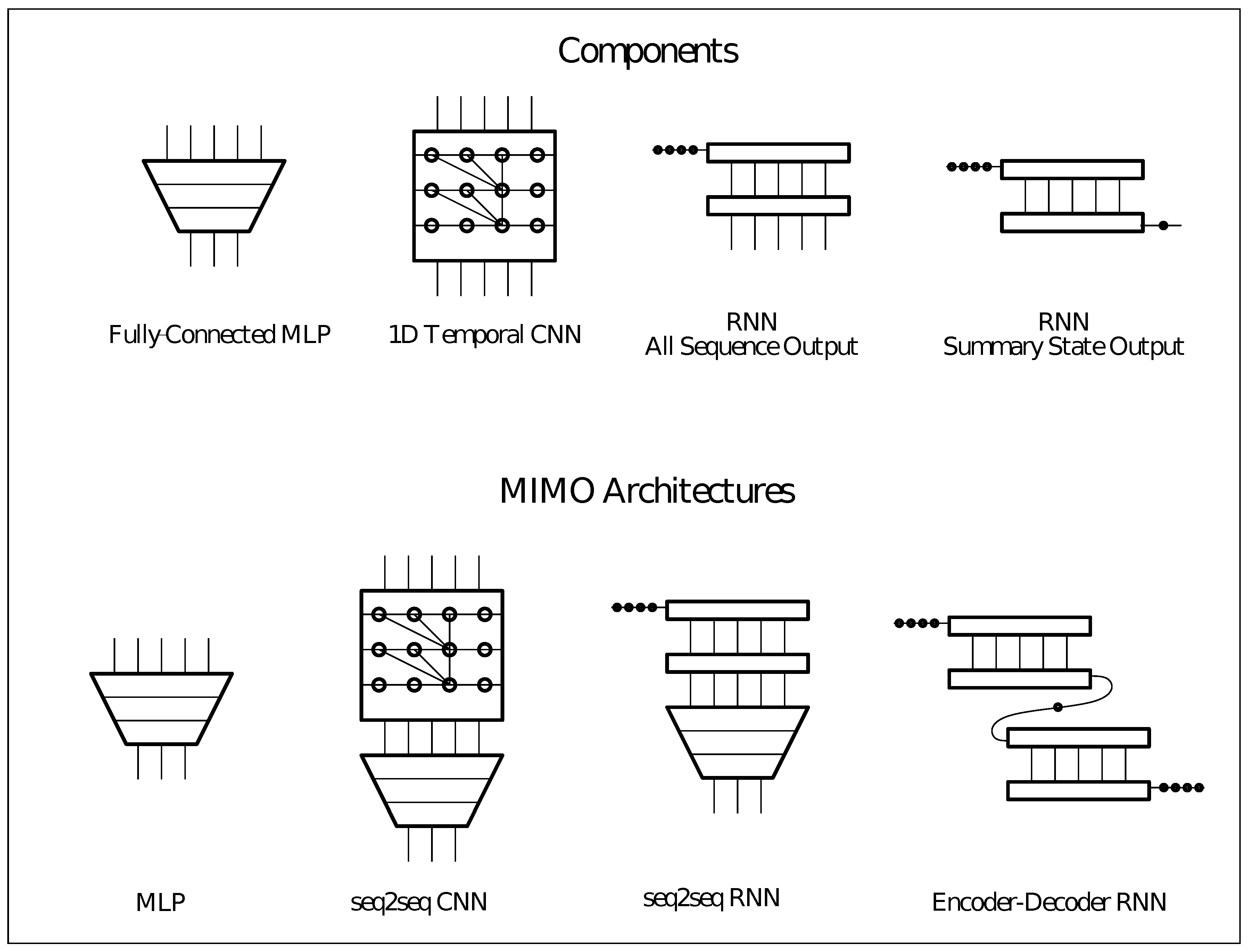
Architectures are deep learning neural networks defined either with direct or with seq2seq (see Section 2.2) approaches. These architectures are built up from four components (see Figure 1).

• Fully-connected MLP
• CNN 1D temporal architecture
• RNN all sequence output
• RNN summary state output

With combinations of these components, 4 architectures were developed: a deep MLP with fully-connected layers (MLP), a CNN combined with an MLP to obtain a sequence output (CNN seq2seq), a RNN combined with an MLP that obtains a sequence and a recurrent neural network (RNN seq2seq), and an RNN with the Encoder Decoder mechanism (RNN ED) (see Figure 1 and

Table 3. Mean and standard deviation of each experiment probability distribution.

Architecture	Mean	St. Dev.	Comments
Persistence	2.69	1.95	Some sites have even negative values
k-NN	4.91	1.01	Results from 1000 sites
MLP Dir	6.83	0.8	Results from 1000 sites
MLP seq2seq	7.06	0.79	Results from 1000 sites
MLP seq2seq	7.05	0.81	Results from all sites
CNN seq2seq	6.90	0.81	Results from all sites
RNN seq2seq	6.85	0.81	Results from all sites
RNN ED	6.86	0.81	Results from all sites

).

3.2.1. Multi-Layer Perceptron

The multi-layer perceptron or feed forward network can be considered as the traditional neural network. The MLP network is organized into neurons (sometimes called nodes) and different layers named input (initial layer), hidden (intermediate layers), and output (final layer). All the neurons are fully connected to the next layer, and information flows from input to output; for this reason, these structures are also named feed forward networks. In the nodes, an activation function processes the inputs coming from the previous nodes and calculates the value to propagate to the connected nodes. Different non-linear activation functions can be used, and the best one for this architecture has been chosen by hyperparameter searching (see Section 3.4). For this MLP architecture, the mathematical formulation for a layer of an MLP is:

$${\mathit{x}}^{\mathit{i}}=g^i(b^i+{\mathit{W}}^i{\mathit{x}}^{\mathit{i}-\mathbf{1}})$$

(2)

where i is the $i\mathrm{th}$ layer, ${\mathit{x}}^{\mathit{i}-\mathbf{1}}$ is the vector of inputs from the previous layer, $g^i$ is the activation function of the layer, ${\mathit{W}}^{\mathit{i}}$ is the weight matrix of the neurons in the layer, and $b^i$ the vector for the independent terms, or bias for this layer.

As the number of parameters in these architectures is quite large, a structured strategy needs to be defined to optimize the different components; in this case, a hyper-parameter search (see Section 3.4) for the MLP is performed considering the parameter depth of the network (number of layers), the number of neurons on each layer, the lag of the input examples, and the activation function used.

3.2.2. Convolutional Networks

Convolutional networks are extensively used for image recognition tasks. Their main capacity is the application of filters to matrices of data that specialize in identifying some specific patterns located in small areas of the matrix or image. In addition to the traditional pattern recognition, there have been recent applications of CNN to time series data, by considering the sequences of data as patterns with good results as in [39], and they have been applied with some success to wind speed, as can be seen in [26,27].

Convolutional networks apply a convolution operation allowing the network to focus on local regions of the input. This is obtained by replacing the weighted sums (see Equation (2)) of the MLP network by the convolution. In each layer, the input is convoluted with the filter weight matrix, creating a feature map. The filter matrix moves on the input and computes the dot product between the input and the filter. For a given filter, all the nodes in the layer detect the same pattern or feature (see Figure 1).

In this work, the CNN architecture was developed using the seq2seq strategy, and the proposed architecture combines a CNN and an MLP structure. The first part of the model consists of several layers of CNN that use one-dimensional convolutions with causal padding (causal padding is a filter that generates a dilated causal convolution, which means that at time step t, only the inputs previous to t are used [40]). The output of the CNN layers is connected to an MLP that computes the prediction as multiple regression.

For the CNN architecture, the main parameters optimized in the hyperparameter searching (see Section 3.4) include the number of filters, the stride and the size of the convolution kernels, the number of CNN layers, the number of layers, the number of neurons, and the activation functions in the MLP.

3.2.3. Recurrent Networks

Recurrent Neural Networks (RNN) are feed forward networks able to process sequences. The structure of an RNN layer is similar to the perceptron, but also with connections that span through time. This means that the computations are done to an element of a sequence depending on the computations from previous elements of the same sequence. This architecture is more natural for time series as it assumes a causal relationship among the data.

One of the hard problems for am RNN architecture to solve is to learn long dependencies among the elements of the sequence. In order to reduce the difficulties of training these architectures, additional mechanisms are added to the basic RNN construct. In the current literature, the Long Short-Term Memory (LSTM) cells [41] and the Gated Recurrent Units (GRU) cells [42] are used in most applications of RNNs to sequential modeling problems.

Two different strategies have been defined with recurrent networks in this work, based on the different ways of obtaining multiple outputs from an RNN. The first possibility is to use the same approach as the one used with the CNN architecture using the output of a multi-layer RNN directly. In this case, each time step of the sequence generates an output that can be used as the input of an MLP. The second possibility, called as RNN ED (Encoder-Decoder) ([41]), is composed of two sets of RNN layers. The encoder layers process the input and generate an output from the sequence that summarizes (encodes) their information. This summary is used as the input of the second RNN that generates the output sequentially, so the previously-generated elements influence the next ones. This makes this architecture slightly different from the rest. Instead of generating all the output at the same time, the relationships among the elements of the generated sequence are also used for the prediction.

The hyperparameter search (see Section 3.4) for the RNN and RNN ED is performed on several dimensions like the type of the recurrent units used (LSTM or GRU), the number of neurons on the recurrent layers, or the number of layers. For the RNN seq2seq or RNN network, as it has a final MLP that combines the two outputs, the output MLP model parameters have been optimized by searching for the best combination of layers and neurons. For the RNN ED, given that there are two groups of recurrent layers, different combinations of layers for the decoder and the encoder have been searched in the hyperparameter setting process.

3.3. Error/Accuracy Measurement

Given that predictions are generated for a large number sites and using a large number of method combinations, using a non-standardized measure of error like, for instance, $MSE$ (Mean Standard Error) is not practical because the error values for each site would depend on the specific range of values contained in the time series measures, so it would be statistically challenging to compare results between different sites. To avoid this problem, $R^2$ (coefficient of determination) was used across all the experiments.

This accuracy measure compares the sum of the square of the residuals and the total sum of squares that is proportional to the variance of the data.

The $R^2$ is be characterized as:

$$R^2=1-\frac{{\sum }_{i=1}^N{({\widehat{y}}_i-y_i)}^2}{{\sum }_{i=1}^N{(y_i-\overline{y})}^2}$$

(3)

The experiments calculated the $R^2$ for each time step (hour). In order to perform the sites’ comparisons, an aggregated measure has been defined by adding the individual $R^2$ values for the 12 steps.

Each experiment obtained an error distribution across all the sites. This distribution was then used for statistical analysis and comparisons using sites, methods, and combinations of both.

The data were z-normalized in a pre-processing phase before training (see Section 3.1), and as a consequence, the value obtained for the $MSE$ was also normalized; as a consequence, the $R^2$ was equal to 1 −$MSE$. $MSE$ can be considered an error measure, while $R^2$ is an accuracy measure, where the closer to 1, the more accurate is the result.

This measure has an intuitive interpretation as it represents the proportion of variance of the fitted model relative to the mean of the real curve, which basically tells us how well the model fits the prediction [43]. The values that express a good fit depend on the domain and the specific application, and for this reason, baseline statistical results were calculated beforehand (see Section 4.1); from the results, it is concluded that a value around 7 (being 12 the maximum) (obtained by adding the $R^2$ values for each step) was reasonable, as it was well over persistence and 25% better than the baseline statistical models tested.

In the wind energy literature, other error measures like Mean Absolute Percentage Error ($MAPE$), Mean Absolute Error ($MAE$), or Root Mean Squared Error ($RMSE$) are possibly more common [10], but to perform the statistical comparisons among the different experiments, taking into account the high number of wind sites available and the variability of the values of the wind series, $R^2$ is considered as more adequate.

3.4. Hyper-Parameter Setting Using a Structured Approach

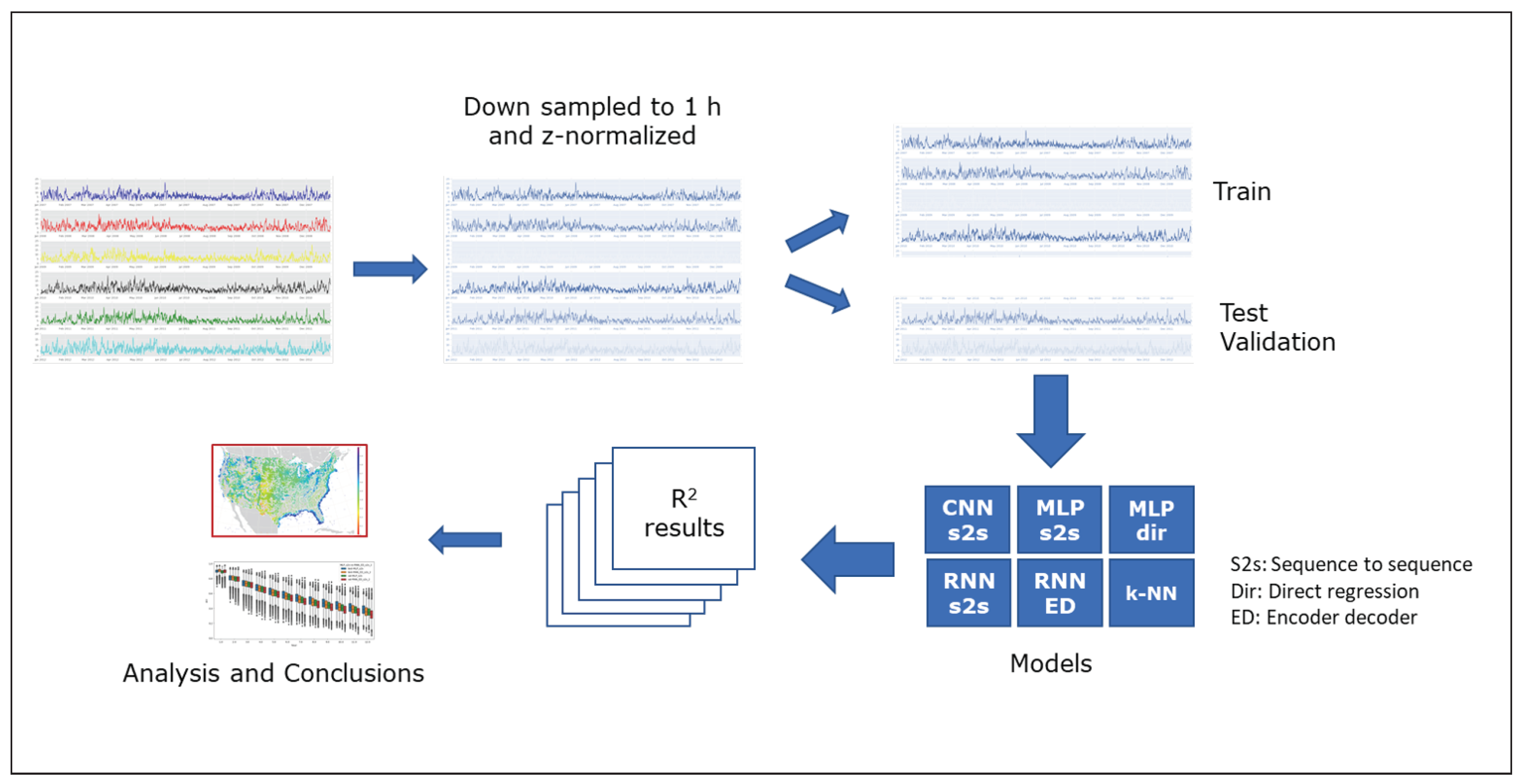
The first activity with each architecture was to find the best hyper-parameter combination. Then, the test executions for all the sites were performed (see Figure 2).

Deep learning uses complex networks, and this generates a very large number of parameter to tune in the experimentation. The exploration of parameters has to be done with a systematic strategy to obtain an effective set of values with the best accuracy. With a small set of parameters, a strategy of manual test and try exploration can be adequate, but with a high number of combinations, we require a more structured approach [44]. In this work, a Sequential Model-Based Optimization (SMBO) strategy has been defined for the hyperparameter setting search. Specifically, the algorithm chosen is an adaptation of the Sequential Model-Based Algorithm Configuration (SMAC) developed by Hutter et al. in [45]. This implementation consists of a structured approach to the hyperparameter setting that assures the generation of a good parameter configuration set in acceptable time. It has been selected for its proven effectiveness and for its capability to manage parameters that have categorical values.

The Bayesian strategy consists of setting a quality criterion and estimating from the results of the parameter combinations a function for this criterion able to predict the quality of new candidate parameters. This function is used to guide the exploration of the configuration space. In this implementation, the sum of $R^2$ for the prediction horizon is used as the quality criterion, and the estimation is obtained using random forest regression ([46]).

Some parameters are manually set like the optimizer, where the choice is an adaptive gradient descent search method (Adamax) [47]. All experiments have limited the number of training epochs to 200 with an early stopping strategy that ends the optimization when the accuracy is not improved for 10 epochs. For a detailed description of each architecture component, see Table 3.

3.5. Some Notes about the Implementation

For the architecture testing, a test-bench has been developed that allows repetition of the experiments using different architectures and parameters over the target dataset or over some selected sites (see Figure 2).

The experiments have been run on the Barcelona Supercomputer (BSC) [32] in a cluster of 39 Nvidia K80 GPUs. Each model trained in 20 s in the CNN/MLP models and 2 min in the RNN. As there were 126,692 sites, the training time was 175 GPU/days for each RNN model and 30 days for each MLP/CNN model. If we include the hyperparameter searching, around 200,000 executions must be added. In total, the estimation was around 600 days of GPU adding all the resources used in this article.

The experimental framework was implemented in Python 3.6 and the deep learning architectures using Keras-Tensorflow [48,49]. Scikit-learn [50] was used for the statistical learning algorithms like the random forest classifier for hyperparameter setting or the k-nearest neighbors to obtain a prediction baseline. Numpy/Scipy [51] has been used for the statistical analysis of the results like the Kolmogorov–Smirnov tests, Tukey’s variance tests, etc.

A copy of the code used for this work is available upon request, with the raw code used to develop the models, and different notebooks with the statistical comparisons and conclusions.

For tuning the models, an iterative structured exploration of the parameter space was applied (see Section 3.4). The final parameter set for each one of the architectures has been tested over the 126,692 wind sites available in the dataset.

4. Results

The research was performed in phases, firstly with the development of a baseline with persistence and statistical learning methods, secondly choosing the best multi-step forecast regression approach between direct and multiple, and thirdly testing the deep learning architectures with the complete set of data. With all the results, a set of statistical analysis has been applied to obtain graphical results and to infer the conclusions presented in this article. The summary of the architectures and their parameter settings can be seen in

Table 4. Architecture details.

Architecture	Description
MLP Dir	MLP with two hidden layers with 1024 and 512 neurons with the ReLU activation function and dropout layers of 0.2 and one output layer with one neuron with linear output. This architecture requires being used as many times as time steps to forecast, 12 times (for horizon 12 h) in this work.
MLP s2s	MLP with two hidden layers with 258 and 128 neurons with the ReLU activation function and dropout layers of 0.4 and one output layer with 12 neurons (equal to the the prediction horizon of 12 h) with linear output.
CNN	One 1D convolutional layer with the ReLU activation function, 256 filters with a stride of 1 and a kernel size of 5, followed by an MLP with an input layer of 32 neurons with the linear activation function and one output layer with as many neurons as the prediction horizon with the linear output, in this case 12, as the horizon is 12 h.
RNN s2s	Two recurrent layers with 32 neurons each, using GRU units with the hard sigmoid recurrent activation function, ReLU activation, and recurrent dropout of 0.1 followed by an MLP with an input layer of 512 neurons with the sigmoid activation, a dropout of 0.1, and a final linear output layer with as many neurons as the prediction horizon, in this case 12, as the horizon is 12 h.
RNN ED	An RNN encoder with two layers of GRU units of 96 neurons and a RNN decoder with one layer of GRU units with 64 neurons both with the hard sigmoid recurrent activation function, ReLU activation function, and a dropout of 0.3, each time step of the prediction horizon being computed with a linear activation function.

.

4.1. Phase 1: Baseline Obtention

Persistence and k-NN have been used as baseline methods for this research. Persistence has been applied to all the sites, but k-NN has been computed for a subset of 1000 sites.

Persistence is the naive method for a time series $〈{\mathit{x}}_1,{\mathit{x}}_2,\cdots ,{\mathit{x}}_n〉$ and uses the value ${\mathit{x}}_n$ as a prediction for a $\widehat{\mathbf{Y}}$ series with horizon H like ${\mathit{x}}_{n+1}={\mathit{x}}_{n+2}=\cdots ={\mathit{x}}_{n+h}={\mathit{x}}_n$.

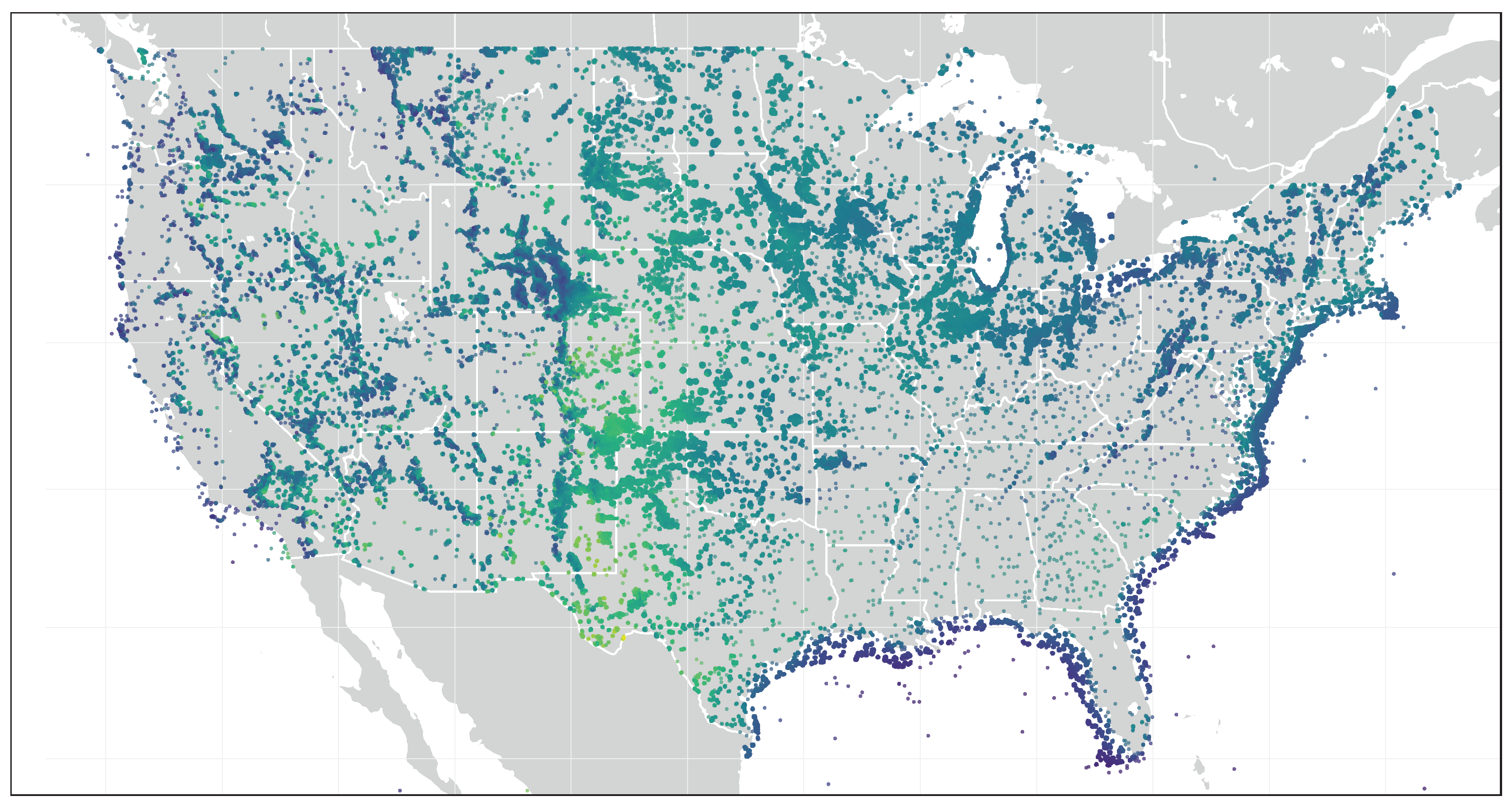
Persistence, as was expected from the literature [10], generated results that showed a steep accuracy $\left(R^2\right)$ deterioration as the time steps increase, becoming negative for some wind sites, indicating inferior predictive results at 12 h. When the results ($\sum R^2$ of each wind site for the 12-h steps) were positioned on a map, the areas with more variability of winds can be observed graphically (see Figure 3); comparing these areas with wind resource studies of the U.S. geography, (like the global wind atlas [52]), it can be observed that where the persistence ratings were rather poor, the variability of winds was very high. The most significant errors were geographically located in areas with complex terrains (Rocky Mountains) and with high wind variability (West Coast and Central Plains). As a result of this comparison, a research question arises. Is the error in persistence an indication of the terrain complexity of the site?

The second experimental baseline consisted of the application of a k-Nearest Neighbors (k-NN) method. For this model, the number of neighbors and the combination of their predictions were explored. The best k-NN model used pre-processed examples data with time windows of 6 h in length, with 15 nearest neighbors (applying Euclidean distance) and with prediction obtained by unweighted averaging of the next 12 h of each neighbor. The baseline k-NN accumulated accuracy results (adding the accuracy of the 12 steps $\sum R^2$) were 4.91 on average, much better than persistence, but with worse results than the DL architectures, as can be seen in the next sections.

Auto-regressive or moving average methods have been discarded, as they cannot cope with the wind time series non-linearity.

4.2. Phase 2: Multi-Step-ahead Regression Strategy Comparison

Section 2.2 describes different strategies for a multi-step-ahead forecast. The objective of this phase is to analyze the best regression approach for the wind forecasting problem, which can be the direct, recursive, simple regression, and multiple regression or sequence to sequence (seq2seq) method. The direct regression is compared to the sequence to sequence approach, while the recursive approach has been discarded based on literature conclusions that have already concluded that it has poorer accuracy when compared with direct regression [34].

An experiment with the MLP architecture was developed to test the two approaches (direct and seq2seq regression). The experiment consisted of an execution on 1000 sites (architectures of two layers in depth and examples with a lag of 12).

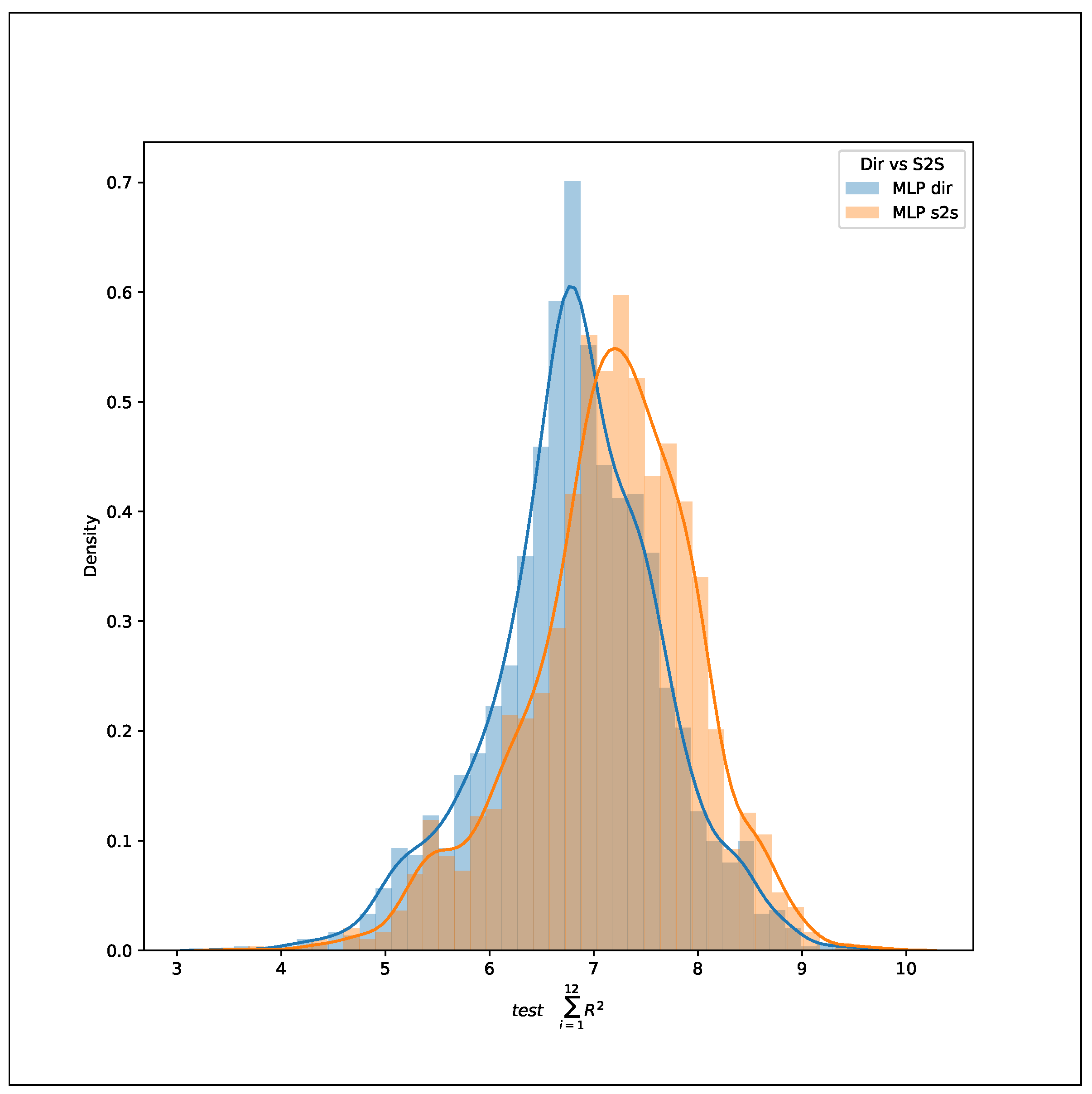
The distributions obtained by the two approaches were quite close, and in order to determine if they were statistically comparable, a Kolmogorov–Smirnov test for equality of the distribution was performed, which obtained a result statistic = 0.175, p-value = 0.0037. With this results, we can conclude that the distribution predictions were not identical and could be compared.

The comparison determined that the seq2seq approach was slightly better, and taking into account the higher computational requirements (as every step in the horizon prediction required an individual model) for the direct regression, the conclusion was to use the seq2seq approach in all the models. This decision was aligned with other research works found in the literature like [53].

Figure 4 offers a graphical comparison of the distributions.

4.3. Phase 3: Deep Learning Model Result Analysis

Four major approaches were finally chosen from the experimentation, Multi-Layer Perceptron seq2seq (MLP), Convolutional Network seq2seq (CNN), Recurrent Neural Network seq2seq (RNN), and Recurrent Network with the Encoder-Decoder architecture (RNN ED), and the experimental architectures parameters have defined by hyperparameter searching using a selection of controlled sites and then tested with the whole dataset (see Section 3.4).

The question to answer is: Which method performs best? After performing all the experiments, a set of result distributions was obtained (see Table 3 with the average results). A $R^2$ probability distribution for each model is obtained, as it can be seen for MLP in Figure 5.

The first issue would be how to compare the different distributions, and this was accomplished by performing an Analysis Of Variance (ANOVA) test, which determines if there are significant statistical differences between the means of all the obtained distributions.

The test result obtained an F-value of 2.655 and a p-value of 0.0317, meaning that there were significant differences among the group of means. To assess the individual differences, Tukey’s honestly significant difference test was performed (see

Table 5. Distribution comparison between the experiment using Tukey’s honestly significant difference test, Family wise error rate $FWER$ = 0.05, after the ANOVA test of a F-value of 2.655 and a p-value of 0.0317.

Group 1	Group 2	Meandiff	Lower	Upper	Reject
CNN	MLP	0.1485	0.1402	0.1568	True
CNN	RNN	−0.0566	−0.0649	−0.0483	True
CNN	RNN ED	−0.0409	−0.0491	−0.0326	True
MLP	RNN	−0.2051	−0.2134	−0.1968	True
MLP	RNN ED	−0.1894	−0.1976	−0.1811	True
RNN	RNN ED	0.0158	0.0075	0.0241	True

). This test compares the distributions assessing the pair differences.

The results showed the MLP method as the better overall one, with a more significant positive difference in the mean compared to the other methods. CNN was better than both RNN variations while RNN encoder-decoder was marginally better than RNN sequence to sequence. From the closeness of the results, it was observed that the worse and best models were not very far from one another.

It could seem counter intuitive that recurrent models do not have the best performance in this domain given that they are specifically tailored to process sequential data. There has been recent literature questioning the necessity of recurrent models in certain domains including time series prediction where long dependencies are not needed [54,55] or because the recurrent models used are stable (no gradient problems during the optimization) and can be approximated by feed forward models [56]. Some feed forward and convolutional architectures have been shown also to outperform recurrent architectures in tasks like automatic translation [57] and speech synthesis [39].

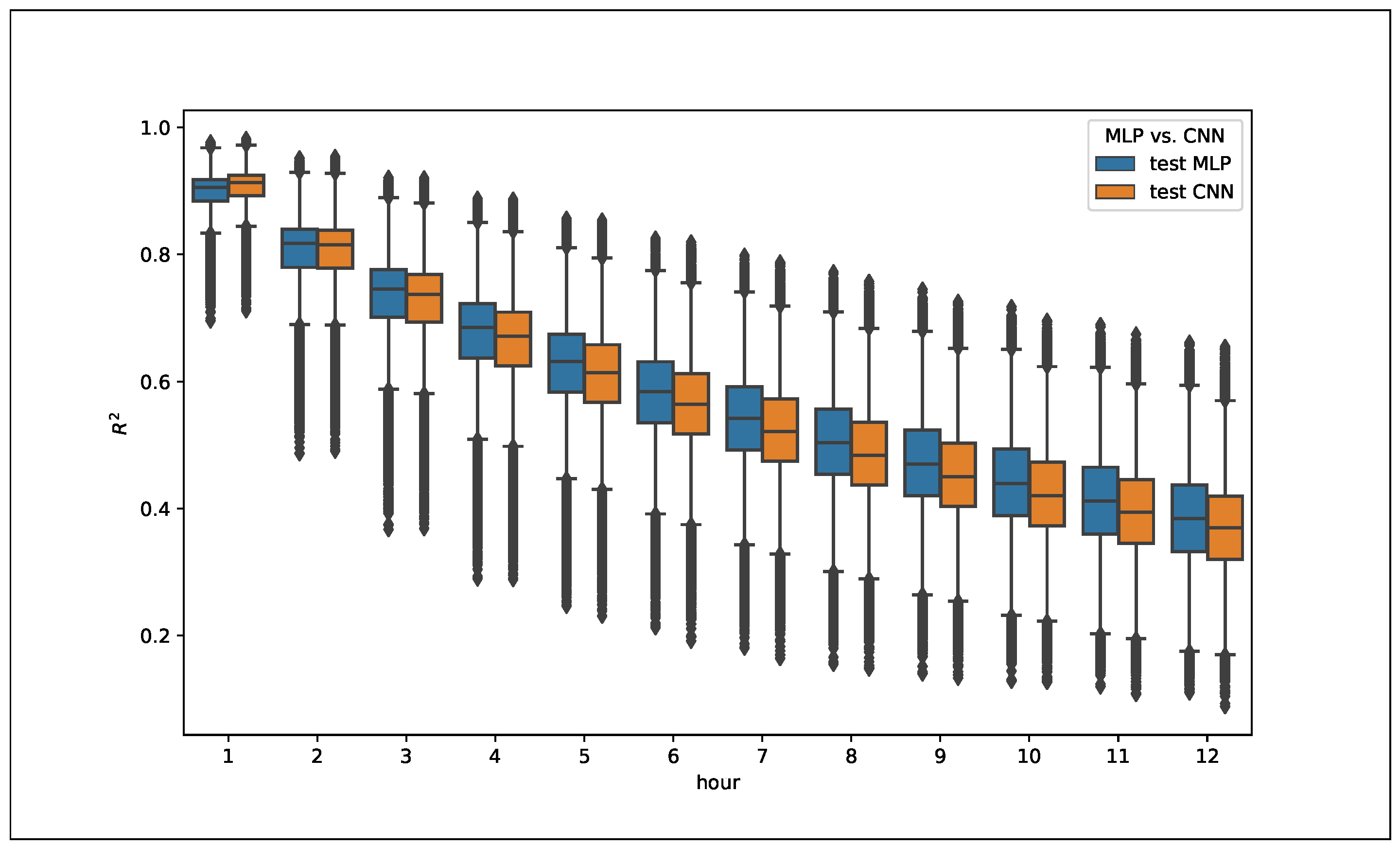
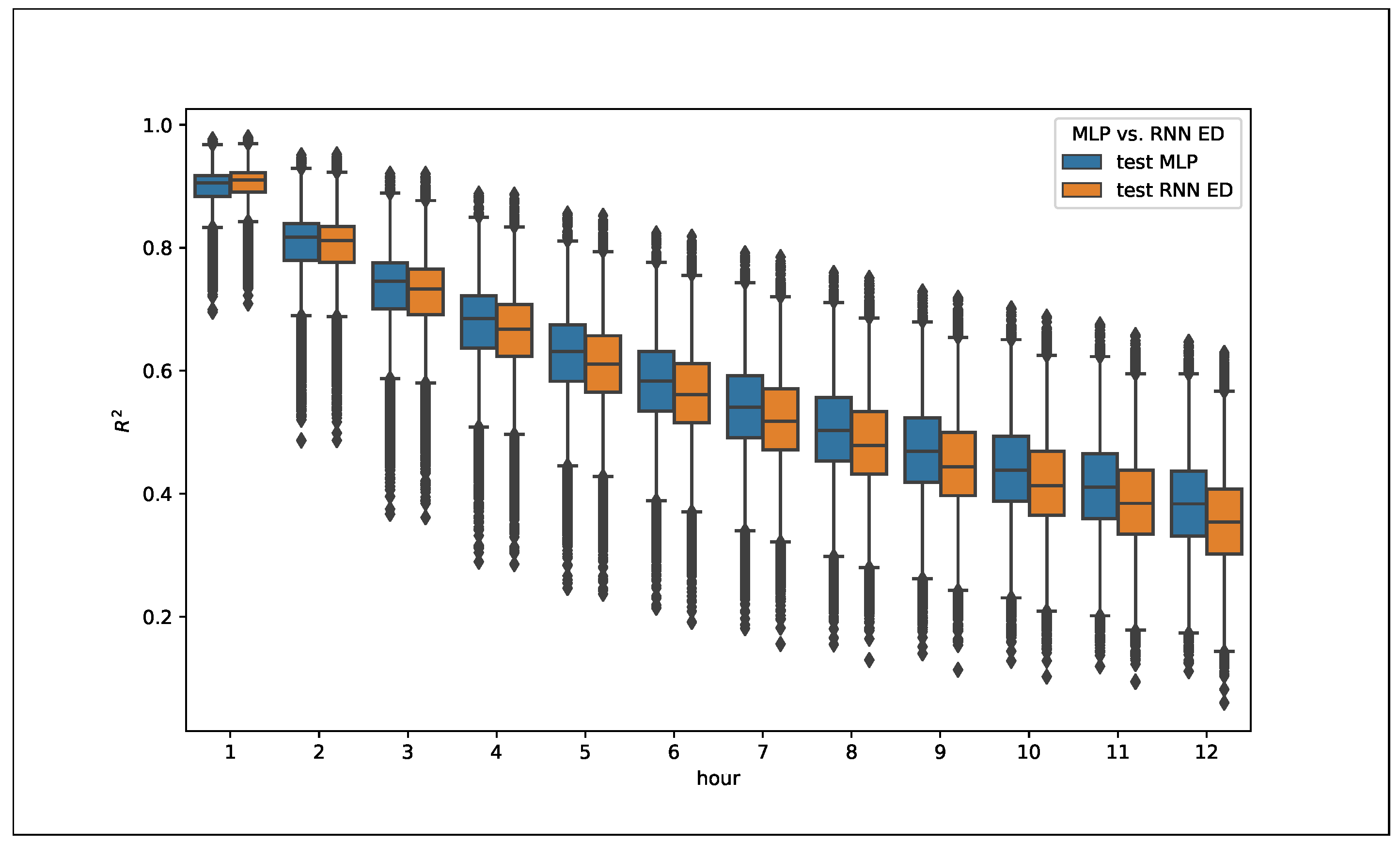
A boxplot of the distribution of $R^2$ for each time horizon (see Figure 6 and Figure 7) show also some relevant characteristics. The RNN and CNN models performed better in the short term (1–2 h) than the MLP ones, which showed better results in the 3–12-h interval. In this sense, it is observed that RNN and CNN are better at learning the short-term characteristics of the series, while MLP is more consistent in the full 12-h prediction. Again, the differences were small, but relevant, as calculated on the 126,692 sites, and showed a valid trend.

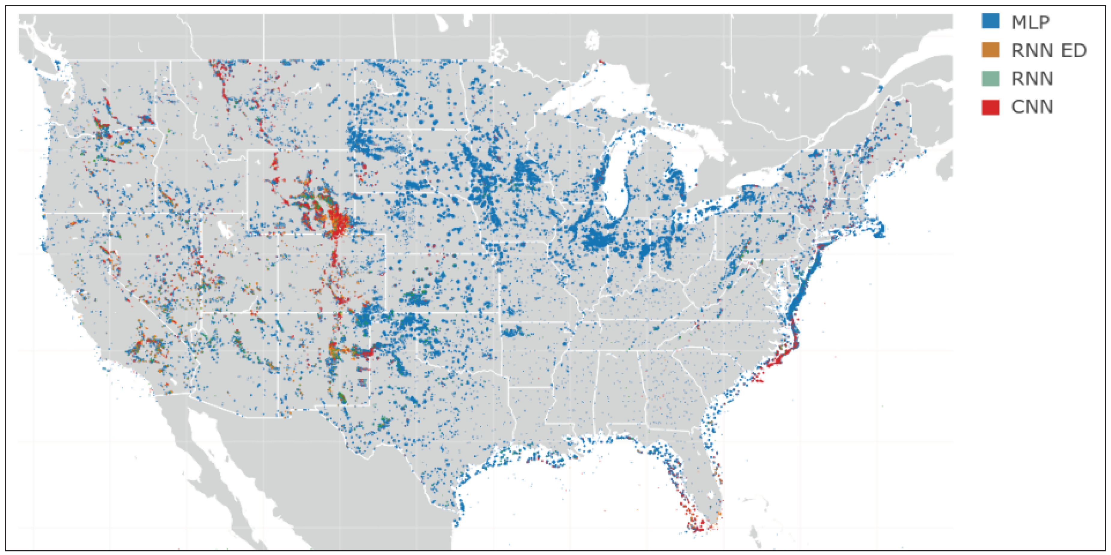
A map of the persistence accuracy across the North America geography has been presented (see Figure 3), and with all the experimental results obtained, a new map was developed showing the best architecture for each wind site (see Figure 8), allowing a graphical analysis of the results to identify geographical patterns related to architectures.

• MLP showed better accuracy in most places
• CNN showed the best accuracy in the Rocky Mountains and the Florida and North Carolina Atlantic Coastline.
• RNN (encoder-decoder) and RNN seq2seq became the best methods in the western area of the U.S. between the Rockies and the Pacific West Coast, especially in the Nevada and Arizona deserts.

From the information on the comparison map (see Figure 8), a relationship between site location (terrain and local characteristics) and the best model can be drawn. This relationship opens up some possible new areas of research, which are analyzed in the conclusions, Section 5.

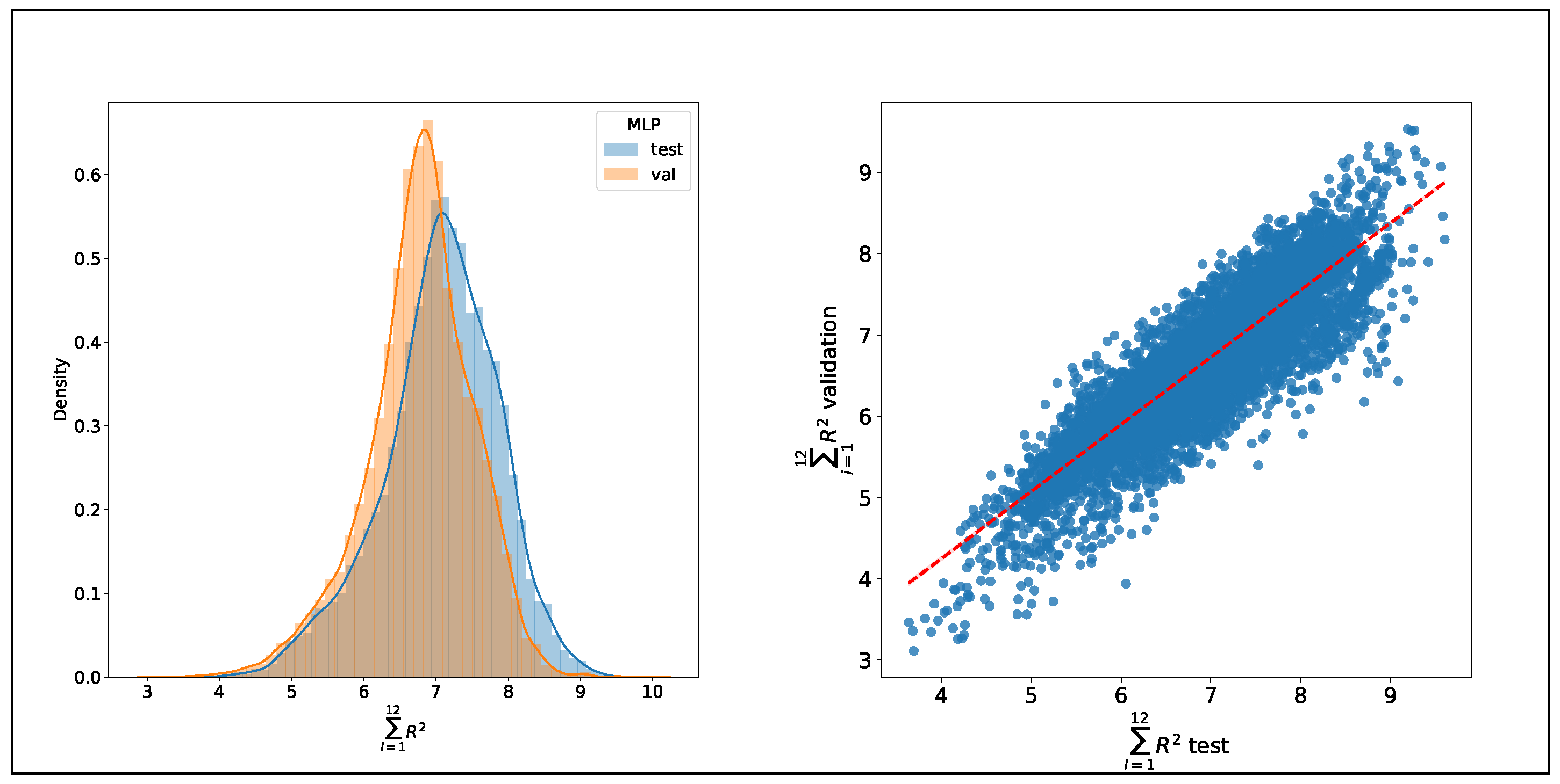
Is the accuracy constant over the years? If there are changes caused by drifting winds, seasonal weather model modifications, and climate change, then the accuracy will vary over time. With seven years of data available, five for the initial training, one year for test, and another for validation, an analysis of the accuracy evolution was made. The comparison between the test and validation datasets that used the sixth and seventh year respectively showed differences in their distributions. In this case, applying a t-test for two related samples, given that the scores were computed for the same population, resulted in a significant difference in means, as can be seen in Figure 5. Computing a linear regression for predicting the validation scores with the test scores, it gave a value of 0.97 for the weight of the test values. This means that even when there is a difference in the mean of the distributions, the model is still consistent, making the initial training still valid. The conclusion is that the wind regime changes slightly on this time frame (seven years), but not enough to interfere with the accuracy of the methods. With this result, it is not possible to establish the variability of wind over time, at least in series of seven years from 2007–2013.

Possibly with longer series, further analysis could be developed, as there are some findings in climatology assuring that wind is speeding up its pattern changes due to the effect of climate change [58].

5. Discussion and Conclusions

In this work, a novel set of projects was developed that implemented and applied deep learning architectures to wind time series. The results and discussion showed that deep learning is a useful prediction tool for wind time series, outperforming other statistical methods for a 12-h-ahead prediction. Forecasting wind speed using methods based exclusively on time series is not a common application, because, for this window horizon, weather forecasting information is usually included; however, this work shows that with the application of deep learning methods, the accuracy improves, with potential to be introduced into the commercial set of tools for wind prediction. The conclusions can be summarized with the following points:

• Deep learning methods showed better accuracy than the baseline statistical methods. This does not come as a surprise as the nature of the task (predicting from time series data only) is extremely difficult for linear statistical modeling.
• The best overall method was MLP seq2seq. This method obtained better averaged results over the whole dataset than the other methods tested. However, the differences between the methods were very small.
• MLP showed better overall results, but if a comparison hour per hour was performed, CNN and RNN outperformed MLP for the short-term prediction (i.e., less than two hours).
• There were geographical areas where one method performed better than the others, showing the geographical dependency between local wind behavior and the best method.
• The best architectures were not very deep, as the best results have been obtained by not very large architectures (number of neurons and layers).
• The optimal length of examples was 18, a result that concludes that series do not need to be very long to be useful; however, more examples will help to improve the networks. This limited number of examples may explain why the RNN and CNN were slightly worse than MLP, as they needed larger amounts of data

These conclusions sustain the affirmation that deep learning algorithms obtain meaningful results in the wind prediction task. They obtain consistent results in 12-h-ahead prediction, beating other traditional methods. The results have generated some new insights into understanding wind time series and open a discussion on how the results can be improved with more complex architectures.

The first alternative, taking into account the geographical-spatial relationship of methods and sites, would be to assemble different methods for each site, to obtain real improvements in accuracy [59] using the best method for each architecture. This way, the overall accuracy improves. Another ensemble development would be to integrate different methods for specific timelines; this would mean that a 12-h-ahead prediction will improve with the CNN/RNN input for the first hours, while MLP would be the main contributor from the third to the twelfth hour, and by increasing complexity in the approach (using a different method for each hour), a better accuracy result will be obtained overall.

One issue in the whole experimental process is that the data available were only seven years long. This length can be considered as too short to learn from the complexity of a wind time series. The data requirements of the deep learning algorithms, which perform better with very rich and long inputs, may require more extended time series. As can be seen in Section 3, the best performing models were not very deep, as a response to the mentioned data availability. To obtain the full value of the deep learning application, longer series are required, but as has been already discussed in Section 2.4, larger sets of real data are not available for research. The optimal length of wind time series to be used for deep learning has to be determined, as wind patterns change over time. This goal can be an interesting area for further research.

This work has been done at the individual wind site (or turbine) level, but further work could be performed developing models integrating sites located in the same areas, taking into account that energy is not generated at isolated sites, but on wind farms that can be quite large. Wind farms have additional dynamics due to two facts, the wake effect, which consists of the impact of the changes in wind by the upstream turbines that impact the others downstream, or the technical loses in the park due to connection issues, distances, or electricity transformation issues. By aggregating sites in clusters or farms, more data examples can be obtained for training, and this fact will open new possibilities for the application of deep learning, like the ones proposed in [15].

As a final conclusion, this work shows the validity of deep learning approaches for wind forecasting, conclusions obtained with the application of the models to wind sites distributed in all the North American geography. The variability of the 129,692 sites assures that the conclusions are based on data that contain all the possible real wind conditions.

Wind energy generation is a growing area that will see a steep increase in the near future, and this growth will increase the need to introduce novel deep learning tools to facilitate the management and control of the energy generation. Energy prediction with deep learning models will be a relevant application that will help the generation of periodical, accurate, and efficient forecasts of future electricity generation.