Multivariable Regression Equivalent Model of Interconnected Active Distribution Networks Based on Boundary Measurement

Abstract

With the increasing complexity of the active distribution network (ADN) due to distributed generation (DG) integration, together with the electricity market evolution, the traditional ADN is divided into multiple areas to operate independently. Due to technical problems or business privacy, the internal network regional control center cannot grasp the changes of the external regional network in time. In order to accurately reflect the distribution network operation state, a multivariable regression equivalent model is proposed in this paper. Firstly, the external network is made equivalent to a multi-port Norton model. The multivariable linear regression model is then derived based on the equivalent distribution network, and the regression model variables are constructed using boundary node information collected by the measurement equipment. Finally, the maximum likelihood estimation (MLE) is used to estimate the parameters of the multivariable linear regression model. Furthermore, case studies demonstrate the effectiveness and robustness of the proposed method, and detailed information of external ADN is unnecessary, except for the boundary node information. The proposed method can also be applied for three-phase unbalanced ADN efficiently.

1. Introduction

Due to the penetration of a large number of distributed generation (DG) in the distribution system, together with demand-side interaction enhancement, the traditional distribution network is gradually evolving into an active distribution network (ADN), and its topology and power flow are moving towards complexity and diversification [1]. In order to reduce the complexity of the distribution network model, together with the electricity market reformation, a single distribution network may be divided into interconnected distribution networks that are operated independently by different owners [2,3]. Due to technical issues or business privacy, information between regions cannot be exchanged in a timely and efficient manner. In order to give the regional management centers the required responsiveness, it is necessary to establish an equivalent method for the three-phase unbalanced interconnected distribution network. The multi-microgrid (MMG), defined as multiple interconnected small-scale power grid that is comprised of distributed energy resource systems, storage devices, and local demands, also has similar characteristics as the interconnected ADN [4,5]. Therefore, the established equivalent method of the interconnection ADN could also be applicable for MMG.

Various equivalent models have been proposed. The Ward equivalent model, REI equivalent model, and their expansion have been widely used [6,7,8,9,10]. However, detailed grid information of the external system is needed by these methods, which cannot make an equivalent for an unknown external system. In practice, to deal with this circumstance, the connected parts of boundary nodes were treated as loads, generators, or a combination of the two when constructing the equivalent model [11,12,13]. However, these methods ignore the coupling relationship among the interconnected external networks, which would lead to large errors when a strong coupling relationship among interconnected grids exists.

Therefore, more accurate equivalent models are needed to reflect the external network information. In [14,15,16,17], the external network equivalent models were built by acquiring the load data of each port, and good results were obtained. However, these models can be used for a single-phase system only, and cannot be applied to the equivalent modeling of three-phase systems. In [18,19,20], Thevenin’s theorem was used to make external network equivalence of multiphase transmission systems to study the transmission performance under different operating conditions. However, when the measurement interval is small and the number of conditions is large, the output may be unstable. The previously mentioned defects were well solved by the deployment of phasor measurement units (PMUs) in [21,22,23,24,25], but the proposed methods are only applicable to power transmission systems, and cannot be used for distribution networks with DGs. As for active distribution systems, equivalent models for the external system were established based on the data acquired by PMUs in [26,27]. A gray-box equivalent model of the external distribution network was conducted in [28]. In [29], the accuracy of the equivalent model was further optimized from the perspective of the reactive power response factor. However, the mentioned equivalent methods are appropriate for three-phase balanced distribution networks with a single port, but not applicable to interconnected three-phase unbalanced distribution networks.

Therefore, an equivalent model for interconnected ADN is proposed in this paper, which is suitable for three-phase balanced and three-phase unbalanced ADN. The contributions of this paper are as follows: (1) In order to enhance the adaptability of the method, a multi-port Norton equivalent model considering the coupling relationship of interconnected networks is proposed. (2) Regarding ADN with unknown external network information, a multivariable linear regression analysis-based method is developed. The multivariable regression model is strictly derived, and the parameters of the multi-port Norton equivalent model of interconnected ADN are estimated using boundary node measurement data. Furthermore, the external system can be a three-phase unbalanced system with unknown topology and state information. (3) For the equivalent accuracy in the operation process of ADN, the boundary information (i.e., complex current, complex voltage) flowing into the external system are selected as regression variables, which are fitted based on the maximum likelihood estimation. The fitting results are used as the external equivalent network parameters, which give the constructed equivalent model a certain dynamic adaptation characteristic.

The rest of the paper is organized as follows: In Section 2, the multivariable regression equivalent model for interconnected ADN is proposed. In Section 3, the estimation procedures of the regression model parameters are introduced. In Section 4, simulations are conducted and analyzed. Finally, conclusions are drawn in Section 5.

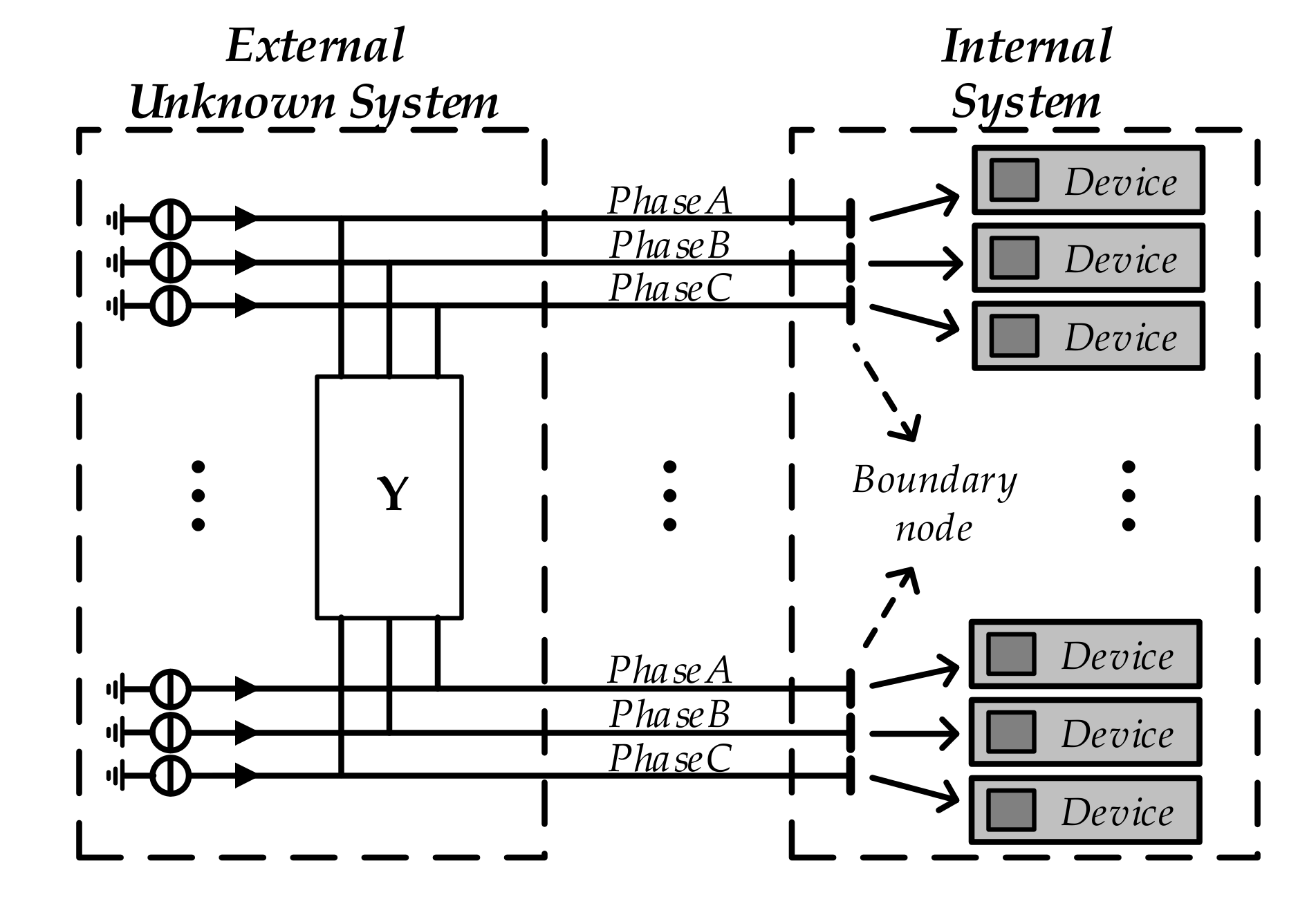
2. Multivariable Regression Equivalent Model

According to circuit principles, external networks connected with the internal network can be equivalent to multi-port Norton models, as shown in Figure 1. And the external Norton equivalent model consists of multiple current sources and admittance matrices [30]. U_E and U_B represent external node voltage and boundary node voltage matrix, respectively. Y_EE and Y_EB represent the external admittance matrix and the external-boundary admittance matrix, respectively. I_E and I_BE respectively represent the Norton equivalent current sources and the outputting current matrix from boundary nodes to external nodes. When the interconnected external grid is a three-phase system, the dimension of these matrixes would be expanded to three times that of the original matrix. Besides, the node number of external systems established by the equivalent model equals the number of boundary nodes.

According to circuit principles, the network equations described by an admittance matrix of the power system can be represented as:

$$[\mathit{Y}][\mathit{U}]=[\mathit{I}]$$

(1)

The network is divided into the internal node set {N}, the boundary node set {B}, and the external node set {E}, then Equation (1) can be re-expressed as:

$$\left[\begin{array}{ccc}{\mathit{Y}}_{\mathit{EE}}& {\mathit{Y}}_{\mathit{EB}}& \\ {\mathit{Y}}_{\mathit{BE}}& {\mathit{Y}}_{\mathit{BB}}& {\mathit{Y}}_{\mathit{BN}}\\ & {\mathit{Y}}_{\mathit{NB}}& {\mathit{Y}}_{\mathit{NN}}\end{array}\right]\left[\begin{array}{c}{\mathit{U}}_E\\ {\mathit{U}}_B\\ {\mathit{U}}_N\end{array}\right]=\left[\begin{array}{c}{\mathit{I}}_E\\ {\mathit{I}}_B\\ {\mathit{I}}_N\end{array}\right]$$

(2)

The voltage sub-matrix U_E corresponding to the external network in (2) can be eliminated through Gaussian elimination method, and the following linear equation is obtained:

$$\left[\begin{array}{cc}{Y}_{\mathit{BB}}-{\mathit{Y}}_{\mathit{BE}}{\mathit{Y}}_{\mathit{EE}}^{-1}{\mathit{Y}}_{\mathit{EB}}& {\mathit{Y}}_{\mathit{BN}}\\ {\mathit{Y}}_{\mathit{NB}}& {\mathit{Y}}_{\mathit{NN}}\end{array}\right]\left[\begin{array}{c}{\mathit{U}}_B\\ {\mathit{U}}_N\end{array}\right]=\left[\begin{array}{c}{\mathit{I}}_B-{\mathit{Y}}_{\mathit{BE}}{\mathit{Y}}_{\mathit{EE}}^{-1}{\mathit{I}}_E\\ {\mathit{I}}_N\end{array}\right]$$

(3)

Equation (3) contains the information of the internal network and external unknown network. Specifically, Y_BEY_EE⁻¹Y_EB contains admittance information of the external network and I_E contains the external network current information, which is unknown. Besides, the remaining parameters in the equation are known to be associated with the internal network, the following equation can be obtained according to (3):

$${\mathit{Y}}_{\mathit{BE}}{\mathit{Y}}_{\mathit{EE}}^{-1}{\mathit{Y}}_{\mathit{EB}}{U}_B=-{\mathit{I}}_B+{\mathit{Y}}_{\mathit{BN}}{U}_N+{\mathit{Y}}_{\mathit{BB}}{U}_B+{\mathit{Y}}_{\mathit{BE}}{\mathit{Y}}_{\mathit{EE}}^{-1}{\mathit{I}}_E$$

(4)

where Y_EB is the mutual admittance matrix between boundary nodes and external nodes. Since the number of external nodes of the established multi-port Norton model is equal to the boundary node number, and the phase loss portion of the boundary node of the unbalanced system can be further deleted, Y_EB is a nonsingular matrix. Therefore, (4) can be transformed into:

$${\mathit{Y}}_{\mathrm{BE}}{\mathit{Y}}_{\mathrm{EE}}^{{-}1}{\mathit{Y}}_{\mathrm{EB}}{U}_B=(-{\mathit{I}}_B+{\mathit{Y}}_{\mathrm{BN}}{U}_N+{\mathit{Y}}_{\mathrm{BB}}{U}_{\mathrm{B}})+{\mathit{Y}}_{\mathrm{BE}}{\mathit{Y}}_{\mathrm{EE}}^{-1}{\mathit{Y}}_{\mathrm{EB}}{\mathit{Y}}_{\mathrm{EB}}^{-1}{\mathit{I}}_{\mathrm{E}}$$

(5)

Let (Y_EB⁻¹I_E), (Y_BEY_EE⁻¹Y_EB)⁻¹ and (−I_B + Y_BNU_N + Y_BBU_B) be represented by U_E^eq, β, and K, then Equations (3) and (5) can be expressed as:

$${\mathit{U}}_B=\mathit{\beta }\mathit{K}+{\mathit{U}}_E^{eq}$$

(6)

$$\left[\begin{array}{cc}{\mathit{Y}}_{\mathit{BB}}-{\mathit{\beta }}^{-1}& {\mathit{Y}}_{\mathit{BN}}\\ {\mathit{Y}}_{\mathit{NB}}& {\mathit{Y}}_{\mathit{NN}}\end{array}\right]\left[\begin{array}{c}{\mathit{U}}_B\\ {\mathit{U}}_N\end{array}\right]=\left[\begin{array}{c}{\mathit{I}}_B-{\beta }^{-1}{\mathit{U}}_E^{\mathit{eq}}\\ {\mathit{I}}_N\end{array}\right]$$

(7)

Equation (7) is the mathematical equivalent model of the external grid with unknown parameters. It is vital to estimate the unknown parameters to obtain the real operation state.

The following equation is obtained through expanding (6):

$$\left[\begin{array}{c}{U}_1\\ ⋮\\ U_{b-1}\\ U_b\end{array}\right]=\left[\begin{array}{cccc}{\beta }_{(1,1)}& \cdots & {\beta }_{(1,b-1)}& {\beta }_{(1,b)}\\ ⋮& \ddots & ⋮& ⋮\\ {\beta }_{(b-1,1)}& \cdots & {\beta }_{(b-1,b-1)}& ⋮\\ {\beta }_{(b,1)}& \cdots & \cdots & {\beta }_{(b,b)}\end{array}\right]\left[\begin{array}{c}{K}_1\\ ⋮\\ K_{b-1}\\ K_b\end{array}\right]+\left[\begin{array}{c}{U}_1^{\mathit{eq}}\\ ⋮\\ U_{b-1}^{\mathit{eq}}\\ U_b^{\mathit{eq}}\end{array}\right]$$

(8)

where b is the number of boundary nodes.

In order to accurately estimate the unknown parameters in Equation (8), the following model is constructed according to the multivariable linear regression analysis method:

$$\left[\begin{array}{cccc}{U}_1^{(1)}& \cdots & U_{b-1}^{(1)}& U_b^{(1)}\\ U_1^{(2)}& \cdots & U_{b-1}^{(2)}& U_b^{(2)}\\ ⋮& \ddots & ⋮& ⋮\\ U_1^{(n)}& \cdots & U_{b-1}^{(n)}& U_b^{(n)}\end{array}\right]=\left[\begin{array}{cccc}1& K_1^{(1)}& \cdots & K_b^{(1)}\\ 1& K_1^{(2)}& \cdots & K_b^{(2)}\\ ⋮& ⋮& \ddots & ⋮\\ 1& K_1^{\left(n\right)}& \cdots & K_b^{(n)}\end{array}\right]\left[\begin{array}{cccc}{U}_1^{\mathit{eq}}& \cdots & U_{b-1}^{\mathit{eq}}& U_b^{\mathit{eq}}\\ {\beta }_{e(1,1)}& \cdots & {\beta }_{e(b-1,1)}& {\beta }_{e(b,1)}\\ ⋮& \ddots & ⋮& ⋮\\ {\beta }_{e(1,b)}& \cdots & {\beta }_{e(b-1,b)}& {\beta }_{e(b,b)}\end{array}\right]$$

(9)

Equation (9) is the multivariable linear regression model of the interconnected active distribution network. By solving the model, the external network equivalent parameters β and U_E^eq can be obtained to estimate the operating state of the system.

3. Algorithm for Regression Model

The algorithm for the multivariable linear regression model of the interconnected ADN is described in this section. Firstly, the boundary system data are collected by measuring equipment placed at boundary nodes. From the theoretical point of view, the equivalent parameters estimation method of the external network is then derived based on the maximum likelihood estimation. Finally, the estimation procedures are introduced.

3.1. Collection Boundary Nodes Information

Measuring equipment, such as PMUs and micro-PMUs, are placed at boundary nodes to synchronously collect the complex current flowing into the external ADN and the complex voltage of the boundary bus [31,32], as shown in Figure 2. The collected boundary information is transmitted to state estimator to constructed Equation (8).

3.2. Maximum Likelihood Estimation of Equivalent Parameters

Regression vertical outliers and poor leverage points can be suppressed by maximum likelihood estimation to achieve the highest statistical efficiency. When the system has a mean Gaussian distribution measurement noise, the Equation (9) can be expressed as follows:

$$\mathit{U}=\mathit{k}\mathit{\beta }+\mathit{\epsilon }$$

(10)

where U is the set of voltage values collected by the internal system measuring equipment, k is the current flowing into the external ADN, β is the constructed external network information matrix, which is called regression coefficient, and ε is the error vector.

The specific form of ε is shown as follows:

$$\mathit{\epsilon }=\left[\begin{array}{cccc}{\epsilon }_1^{(1)}& \cdots & {\epsilon }_{b-1}^{(1)}& {\epsilon }_b^{(1)}\\ {\epsilon }_1^{(2)}& \cdots & {\epsilon }_{b-1}^{(2)}& {\epsilon }_b^{(2)}\\ ⋮& \ddots & ⋮& ⋮\\ {\epsilon }_1^{(n)}& \cdots & {\epsilon }_{b-1}^{(n)}& {\mathit{\epsilon }}_b^{(n)}\end{array}\right]$$

(11)

The density function of error is as follows:

$$f\left({\epsilon }_i\right)=\frac{1}{\sigma \sqrt{2\pi }}\exp (-\frac{1}{2{\sigma }^2}{\epsilon }_i^2)$$

(12)

where the constant σ² represents the variance.

The maximum likelihood function is the joint density function of ${\mathit{\epsilon }}_1,{\mathit{\epsilon }}_2,\cdots ,{\mathit{\epsilon }}_n$, or ${\mathrm{\Pi }}_{i=1}^{n}f\left({\epsilon }_i\right)$, and its specific form is as follows:

$$\mathit{L}\left(\epsilon ,{\sigma }^2\right)=\underset{i=1}{\overset{n}{{\displaystyle \mathrm{\Pi }}}}\mathit{f}({\epsilon }_i)=\frac{1}{{(2\pi )}^{n/2}{\sigma }^n}\mathrm{e}\mathrm{x}\mathrm{p}(-\frac{1}{2{\sigma }^2}{\mathit{\epsilon }}^T\mathit{\epsilon })$$

(13)

Bring Equation (10) into (13), the likelihood function can be transformed as follows:

$$\mathit{L}\left(\mathit{U},\mathit{\beta },{\sigma }^2\right)=\frac{1}{{(2\pi )}^{n/2}{\sigma }^n}\mathrm{e}\mathrm{x}\mathrm{p}\{-\frac{1}{2{\sigma }^2}{(\mathit{U}-\mathit{k}\mathit{\beta })}^T(\mathit{U}-\mathit{k}\mathit{\beta })\}$$

(14)

For a constant value σ, to maximize the likelihood function, the optimal estimation matrix β is required to minimizing the term ${(\mathit{U}-\mathit{k}\mathit{\beta })}^T(\mathit{U}-\mathit{k}\mathit{\beta })$. And the residual squared function S(β) is introduced:

$$S\left(\mathit{\beta }\right)={\displaystyle \sum _{i=1}^n{\mathit{\epsilon }}_i^2}={\mathit{\epsilon }}^T\mathit{\epsilon }={(\mathit{U}-\mathit{k}\mathit{\beta })}^T(\mathit{U}-\mathit{k}\mathit{\beta })$$

(15)

It is noted that ${\mathit{\beta }}^{\mathit{T}}{\mathit{k}}^T\mathit{U}$ and ${\mathit{U}}^T\mathit{k}\beta$ are the same matrix due to the symmetry of the system admittance matrix, and S(β) can be further expressed as the following equation:

$$S\left(\mathit{\beta }\right)={\mathit{U}}^T\mathit{U}-2{\mathit{\beta }}^T{\mathit{k}}^{\mathit{T}}\mathit{U}+{\mathit{\beta }}^T{\mathit{k}}^T\mathit{k}\mathit{\beta }$$

(16)

Since all columns of the regression variable k obtained according to multiple sets of power flow are not linearly combined with other columns, k is a nonsingular matrix. Hence, the estimated vector of $\widehat{\beta }$ is as follows:

$$\begin{array}{ll}\hat{\mathit{\beta }}& =\arg \underset{\beta }{\min }S\left(\mathit{\beta }\right)\\ & =\arg \underset{\beta }{\min }\left({\mathit{U}}^T\mathit{U}-2{\mathit{\beta }}^T{\mathit{k}}^T\mathit{U}+{\mathit{\beta }}^T{\mathit{k}}^T,\mathit{k}\mathit{\beta }\right)\\ & =({\mathit{k}}^T\mathit{k}{)}^{-1}{\mathit{k}}^T\mathit{U}\end{array}$$

(17)

The obtained $\widehat{\beta }$ is the maximum likelihood estimation parameter matrix, and the detailed solution of the multivariable linear regression model can be found in [33]. The matrix U_E^eq can be obtained by bringing the estimated matrix $\widehat{\beta }$ into Equation (6). Bring $\widehat{\beta }$ and U_E^eq into Equation (7) to establish the multi-port Norton equivalent model of the external system. Thus, the operation state of the interconnected ADN can be effectively estimated accordingly.

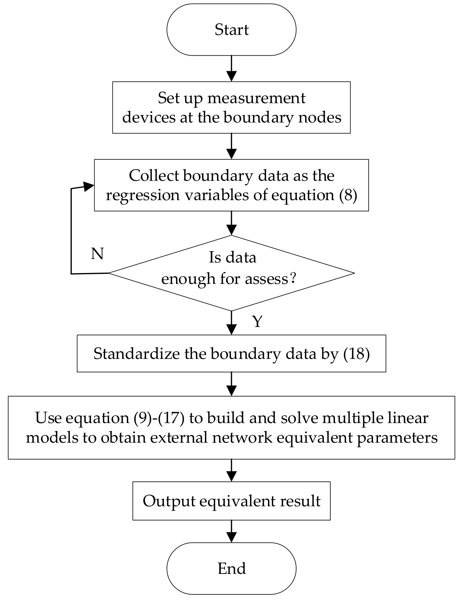
3.3. Equivalent Procedures

The external network equivalent method proposed in this paper consists of two phases. In the first phase, the measuring devices are used to synchronously collect the boundary node data (complex voltage and complex current, see Figure 1). In the second phase, the multiple regression equivalent models are established and solved to obtain the external network equivalent parameters. The external equivalent network is constructed by using the equivalent parameters to reflect the real operating state of the system.

The proposed external network equivalent algorithm can be summarized by the following steps:

Step 1: Set up the measuring devices to synchronously measure the complex voltage U_B and complex current K flowing into the external network.

Step 2: The collected boundary information is used as the regression variable in Equation (8). In order to estimate the external network parameters more accurately, the number of regression variables collected can be referenced to [34].

Step 3: Standardize boundary data according to the following equation:

$${\mathit{x}}^{*}=\frac{x_i-\overline{x}}{\sigma }$$

(18)

where

$$\sigma =\sqrt{\frac{1}{N}{\displaystyle \sum _{i=1}^N{\left(x_i-\overline{x}\right)}^2}}$$

$\overline{x}$ is the average of the collected data, and N is the number of collected data.

Step 4: A multivariate linear regression model is established based on Equation (9), and then the maximum likelihood estimation is used to solve the model based on Equations (10)–(17) to obtain external network equivalent parameters β and U_E^eq.

The external network equivalent procedures are shown in Figure 3.

4. Simulation Verification

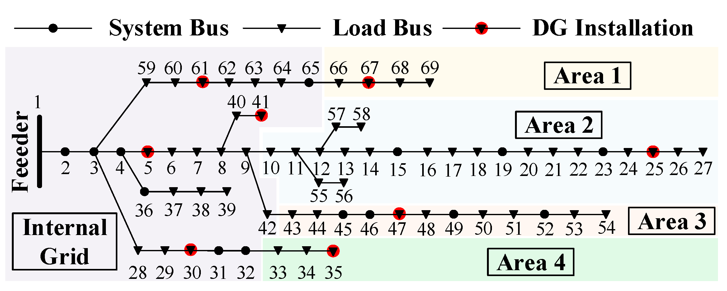
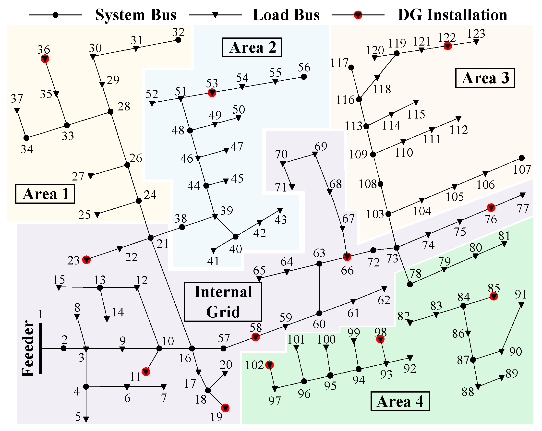
In this section, Matlab and Opendss interactive simulations are performed on the personal computer with a 1.9 GHz A8 processor and 8 GB RAM to verify the accuracy of the proposed algorithm. The method proposed in this paper named MEG is compared with three mainstream equivalent methods: (1) PQ equivalent: The external network is made equivalent to load according to the injected power of the boundary node. (2) PV equivalent: The external network is made equivalent to the generator according to the injected power of the boundary node. (3) COM equivalent: The external network is equivalent to the generator if the injected power of the boundary node is positive, otherwise, it is equivalent to load.

4.1. Test Systems

Simulation on the IEEE 69-node distribution test system and IEEE 123-node distribution test system are carried out to verify the effectiveness and accuracy of the proposed method. The two systems constructed are divided into an external network, boundary network, and internal network, and the node numbers are rearranged, as shown in Figure 4 and Figure 5. The external network consists of various areas with DGs installed.

Case I: The modified IEEE 69-node system is a three-phase balanced system, node 1 is the balanced node, and the initial voltage is 12.66 kV. The three-phase power base value is 10 MVA, and the total load is 3802.19 + j2694.6 kVA [35].

Case II: The modified IEEE 123-node system is a three-phase unbalanced system with a voltage level of 4.16 kV, the relaxation node voltage is set to 1.05 (per-unit value), the feeder capacity is 5.28 MW, the three-phase active power is 3490 kW, and the reactive power is 1925 kVar [36,37].

4.2. Scenarios Setting

The distribution system operator will adjust the operating condition by changing the structure of the distribution system accordingly [38]. Different scenarios are constructed to simulate the operation states of the distribution system based on the two cases above.

4.2.1. Three Scenarios based on Case 1

Scenario 1: modified IEEE 69-node three-phase balanced distribution system with DG integration. Information of installed DGs are shown in

Table 1. Distributed generation (DG) information in Case 1.

Internal Grid			External Grid
Name	Node	P(kW)	Name	Node	P(kW)
DG1	5	71.9	DG5	25	44.3
DG2	30	49.8	DG6	35	66.7
DG3	41	64.3	DG7	47	132.9
DG4	61	173.8	DG8	67	113.8

and the reactive power limits of DGs are [−0.1 Mvar, 0.2 Mvar].

Scenario 2: Based on Scenario 1, the normal loop closing operation is performed, and the nodes connected by the loop closing interconnection switch are node 15 and node 69.

Scenario 3: modified IEEE 69-node distribution system with random fluctuation load. It is a dynamic scenario, and the load curve is shown in Figure 6.

4.2.2. Three Scenarios based on Case 2

Scenario 1: modified IEEE 123-node three-phase unbalance distribution system with DG integration. The information of installed DGs are shown in

Table 2. DG information in Case 2.

Internal Grid				External Grid
Name	Node	Phase	P(kW)	Name	Node	Phase	P(kW)
DG1	11	B	16.3	DG7	36	C	82.6
DG2	19	C	20.1	DG8	53	A	184.9
DG3	23	A	18.0			B	202.1
DG4	58	A	12.3			C	303.3
		B	32.9	DG9	85	A	64.3
		C	62.9			B	77.2
DG5	66	A	42.3			C	67.5
		B	32.9	DG10	98	A	92.9
		C	62.9	DG11	102	B	62.9
DG6	76	C	67.3	DG12	122	A	51.6

and the reactive power limits of DGs are [−0.1 Mvar, 0.4M var].

Scenario 2: Based on Scenario 1, the normal loop closing operation is performed, and the nodes connected by the loop closing interconnection switch are node 56 and node 117.

Scenario 3: This is a dynamic scenario based on Scenario 1 with fluctuation load. The load curve is the same as Case I.

4.3. Equivalent Error Indicators

Since the basic requirement of the distribution system is to provide reliable voltage support for the demand, the voltage related indicators are used in this paper to evaluate the accuracy of the equivalent methods. The average absolute error e_avg and the maximum absolute error e_max of the node voltage amplitude are selected as the indicators during the static simulation scenarios, and expressions are as follows:

$$\left\{\begin{array}{c}{e}_{\mathit{max}}=\mathrm{m}\mathrm{a}\mathrm{x}\left\{\right|\frac{V_n-V_n^{\mathit{eq}}}{V_n^{eq}}|\times 100\%,n\in N\}\\ e_{\mathit{avg}}=\mathrm{a}\mathrm{v}\mathrm{g}\left\{\right|\frac{V_n-V_n^{\mathrm{eq}}}{V_n^{\mathit{eq}}}|\times 100\%,n\in N\}\end{array}\right.$$

(19)

where V_n is the voltage value of node n renumbered in the internal network under the original model, V_n^eq is the voltage value of node n under the equivalent model, and N is the internal network node set. The lower error indicators e_max and e_avg represent higher equivalent accuracy.

Under dynamic scenarios, the root mean square error of each node voltage before and after equivalent is used as the measuring indicator. The calculation formula is as follows:

$$V_{\mathit{RMSE}}=\sqrt{\frac{{\displaystyle \sum _{i=1}^m{\left(V_n-V_n^{\mathit{eq}}\right)}^2}}{m}}$$

(20)

where m is the number of collection points within a certain period of time. Lower V_RMSE value obtained under the load fluctuation scenario means higher equivalent accuracy.

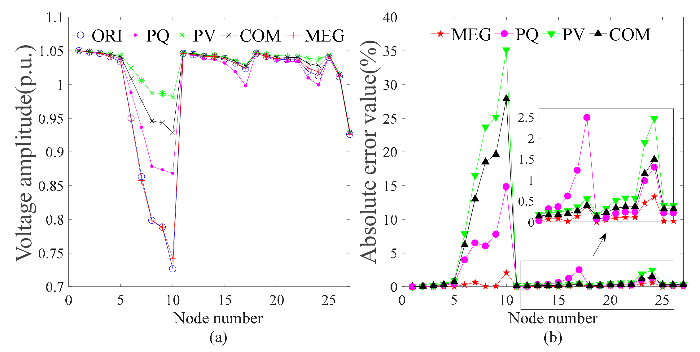
4.4. Simulation Results of Case 1

4.4.1. Scenario 1

Figure 7a and b respectively show the internal system voltage amplitude and the absolute error of four equivalent modeling methods under Scenario 1 of Case 1. ORI depicts the voltage amplitude of the original system. As can be seen from the figure, four different equivalent models can reflect the voltage of each node of the original system to some extent, but the voltage calculated by the method proposed in this paper is closer to the actual value. Which indicates that the proposed equivalent model improves the accuracy dramatically.

Table 3. Equivalent errors of four models with DG and without DG.

Method	Without DG		With DG
	emax (%)	eavg (%)	emax (%)	eavg (%)
MEG	0.48	0.21	1.823	0.03
PV	2.68	0.89	34.68	7.01
PQ	2.45	0.72	19.44	3.18
COM	1.78	0.63	27.34	5.23

shows the equivalent errors values of e_max and e_avg of the four methods with DG and without DG. It can be seen from the table that the equivalent accuracy drops significantly due to the integration of DG, especially for the methods of PV, PQ, and COM. However, the values of e_max and e_avg calculated by the equivalent model proposed in this paper are still relatively small compared with the other three methods, which indicates the robustness and the equivalent accuracy of the proposed method. Hence, the equivalent model proposed in this paper reveals the real situation of the original system.

4.4.2. Scenario 2

Figure 8a,b respectively show the internal system voltage amplitude (p.u.) and absolute error (%) as reflected by the equivalent model obtained by each method in Scenario 2. As can be seen from the figure, after the loop closing, the voltage of each branch connected to the loop closing interconnection switch has a significant drop. The equivalent model obtained by the above four methods can basically reflect the voltage of each node in the original system, but the internal node voltage calculated by the method proposed in this paper is closer to the actual value of the internal voltage of the system.

Table 4. Equivalent errors of four models in Scenario 2.

Error Indicator	MEG	PV	PQ	COM
emax (%)	1.769	26.97	8.07	18.76
eavg (%)	0.17	5.64	1.80	4.68

compares the equivalent results e_max and e_avg reflected by the above four equivalent modeling methods in Scenario 2. As can be seen from the table, under the loop closing state, the internal system voltage e_max and e_avg calculated by the equivalent model proposed in this paper are smaller than those obtained by the other three methods, indicating that compared with the other three models, the model proposed in this paper has a higher equivalent accuracy and can more accurately reflect the voltage states of the internal system.

4.4.3. Scenario 3

Load fluctuations are introduced in this scenario to further illustrate the dynamic characteristics of the proposed equivalent model for interconnected ADN. Figure 9a shows the dynamic variation of the voltage amplitude of each node in the internal network of the original model. It can be seen that the voltage of each node fluctuates slightly with the fluctuation of the load, but can be maintained within a certain range under the action of the relaxed node. Figure 9b shows the absolute error of the internal system voltage obtained by the equivalent model proposed in this paper. It can be seen from Figure 9b that the equivalent accuracy of the proposed method can be guaranteed even in this dynamic scenario (the equivalent error is lower than 1%). It can also accurately reflect the variation of the internal system voltage.

Figure 10 shows the voltage mean square errors (V_RMSE) for four different models before and after equivalent. It can be seen from the figure that under Scenario 3, the V_RMSE value (lower than 2.5%) obtained by the method proposed in this paper is lower than that of the other three methods (greater than 5%), indicating that the equivalent model proposed in this paper can reflect the actual voltage of the internal system under dynamic scenarios better and has better dynamic characteristics.

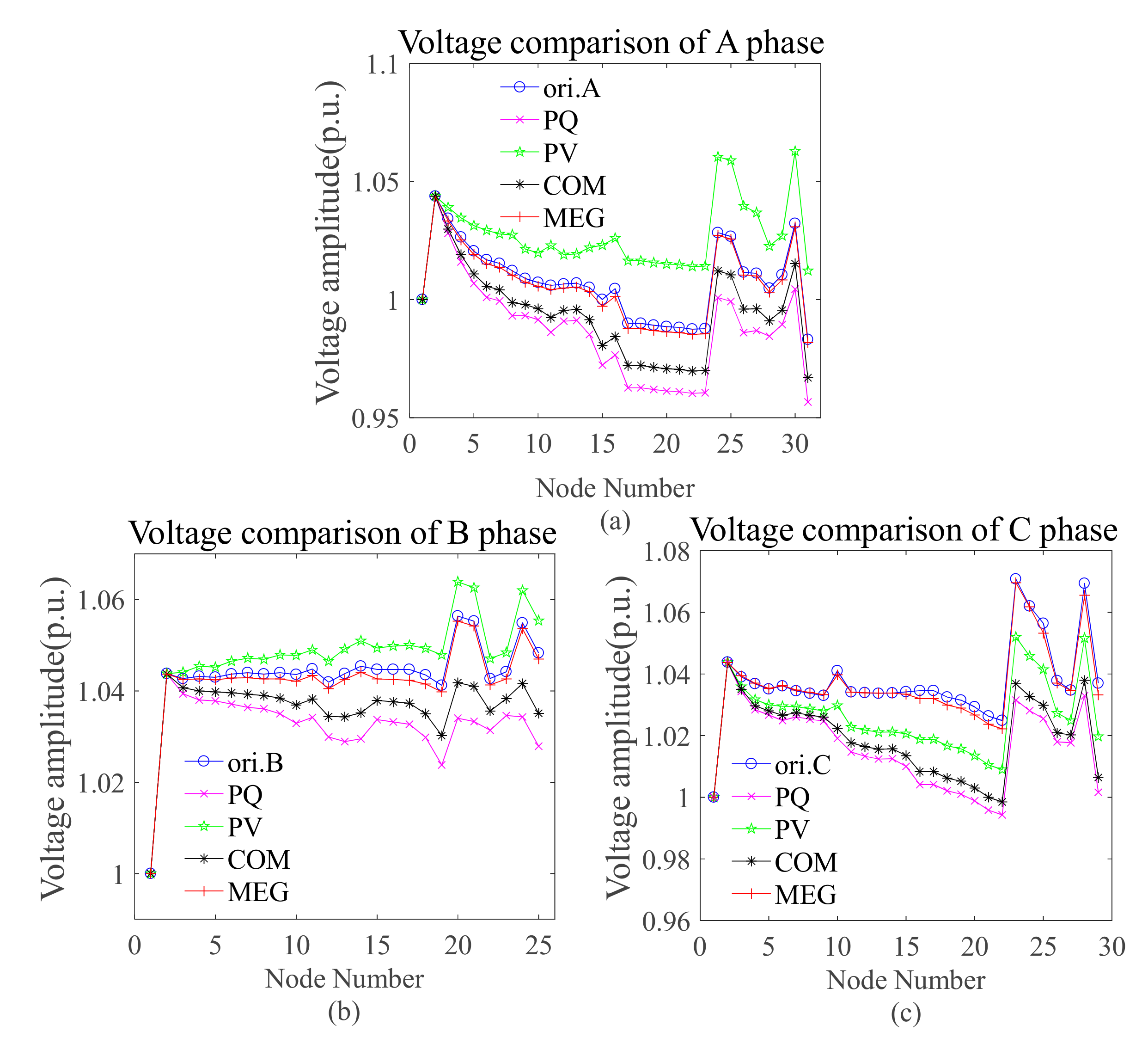
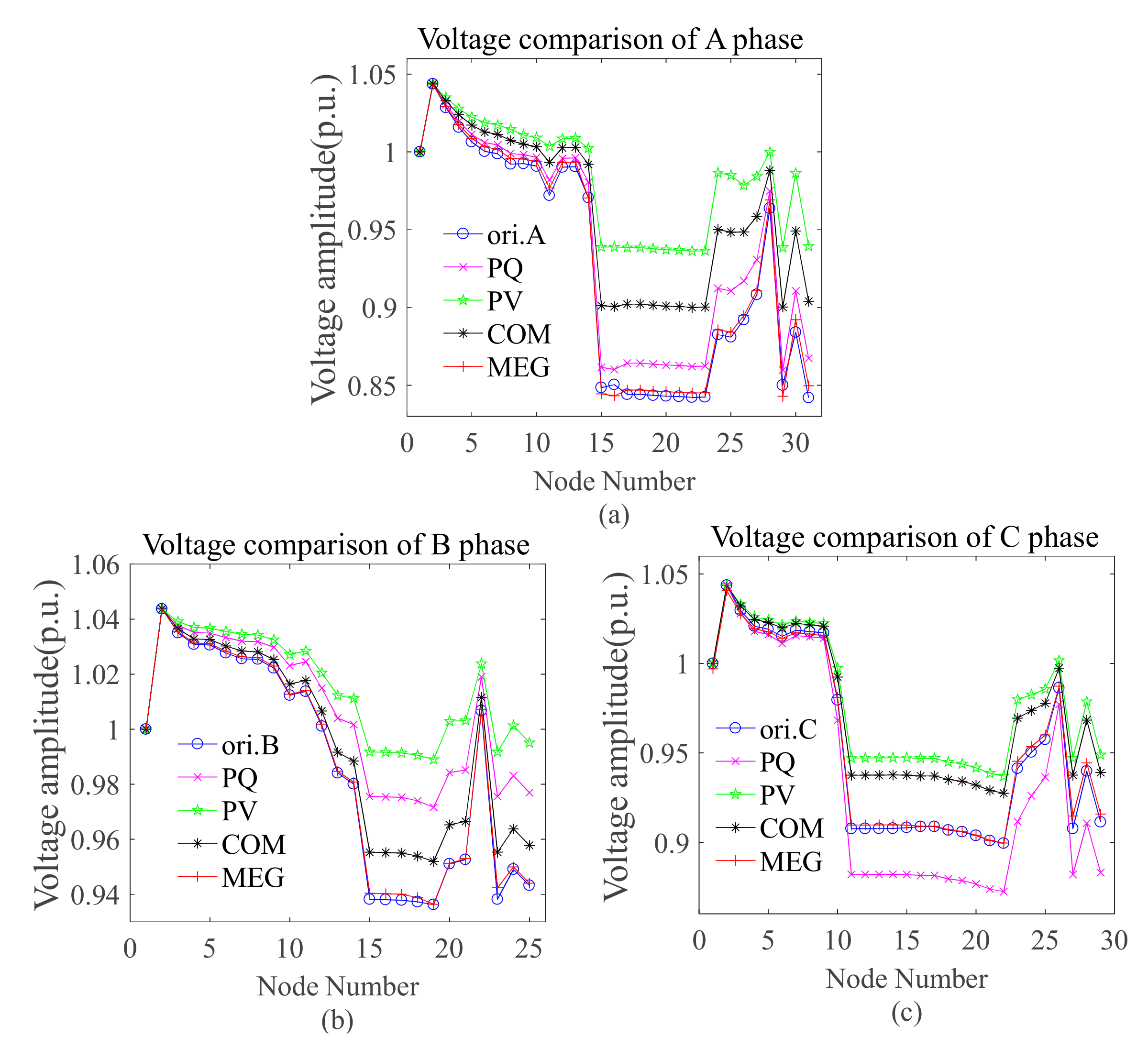
4.5. Simulation Results of Case 2

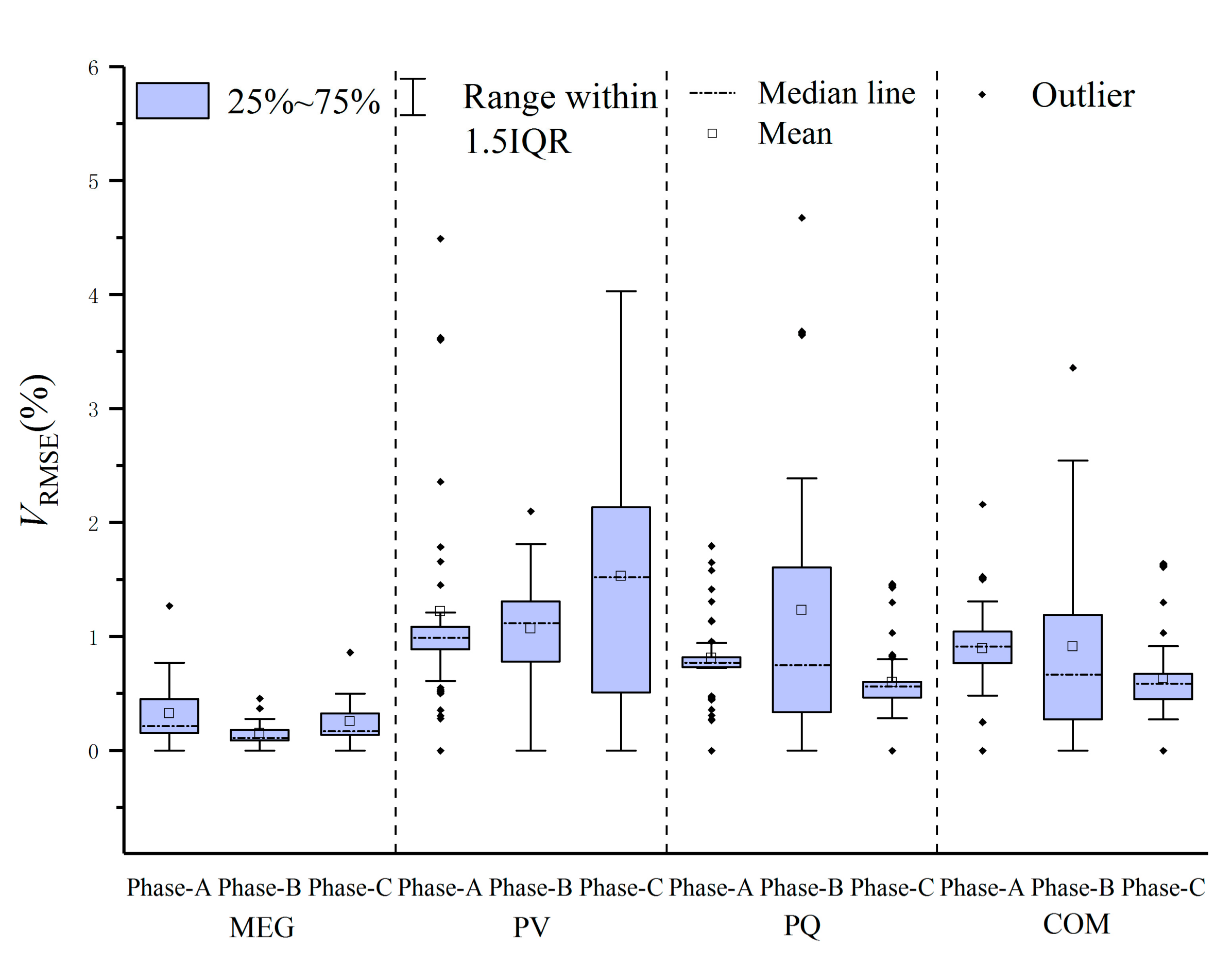
4.5.1. Scenario 1

In Scenario 1, The simulation results with different models are shown in Figure 11a–c, respectively. As we can see, the node voltages obtained by four methods are similar (some nodes lack a phase due to the three-phase unbalance characteristics). However, the voltage amplitude obtained by the method proposed in this paper is closer to the voltage using the original model, which indicates that the equivalent method proposed in this paper can reveal the actual voltage better than the other three methods, when large numbers of DGs are connected to the distribution networks.

The results of e_max and e_avg obtained by four methods are shown in

Table 5. Absolute errors of different models in Scenario 1.

Method	emax (%)			eavg (%)
	A	B	C	A	B	C
MEG	0.33	0.23	0.44	0.16	0.13	0.16
PV	3.15	0.71	1.76	2.13	0.49	1.14
PQ	2.82	2.80	3.67	2.20	1.31	2.21
COM	2.02	1.38	3.18	1.43	0.83	1.89

. It can be seen from the table that the absolute errors of each phase voltage obtained by the method proposed in this paper are the smallest compared with the other three methods, which indicates that the accuracy of the method proposed in this paper is higher.

4.5.2. Scenario 2

Figure 12a–c show the internal voltage amplitude obtained by different methods in Scenario 2. It can be seen from the figure that after the normal loop closing of the distribution system, the phase voltages of the internal system nodes are lower than the complete model. The voltage amplitudes of the nodes connected to the loop-closing line are significantly decreased, and the internal node voltages obtained by the respective methods are close to the original values of the system.

Table 6. Absolute errors of different models in Scenario 2.

Method	emax(%)			eavg(%)
	A	B	C	A	B	C
MEG	1.27	0.44	1.11	0.16	0.13	0.16
PV	11.83	5.71	4.35	6.93	3.40	2.45
PQ	3.37	3.99	3.16	1.78	2.32	1.69
COM	4.82	11.4	7.14	2.76	6.84	4.01

shows the e_max and e_avg of the above four methods in Scenario 2. It can be seen from the table that the equivalent accuracy of the four methods in the loop-opening state is significantly lower than that in Scenario 1. However, the absolute error value of voltage obtained by the method proposed in this paper is still the smallest compared with the other three methods, which indicates that the method proposed in this paper is more accurate in terms of equivalent than the other three methods in the original network loop-opening state, and has the best equivalent accuracy.

4.5.3. Scenario 3

The voltages of three-phase of the internal system using the original model are as shown in Figure 13a–c. As we can see, it shows obvious fluctuation with the load changing. However, the fluctuation is maintained within a certain range due to the existing compensation devices such as capacitors.

Figure 14 a–c shows the absolute error of the three-phase voltage of each node obtained by the equivalent model proposed in this paper. It can be seen from the figure that the maximum absolute error of three-phase voltage is lower than 2%, which indicates that the accuracy of the proposed equivalent model can be assured even under the dynamic scenario with fluctuation load.

Figure 15 shows the value of V_RMSE using different equivalent models. It can be seen that the V_RMSE of the internal nodes of each phase obtained by the method proposed is the smallest with dynamic fluctuation load, and the V_RMSE of three-phase is less than 0.5%, which indicates that the equivalent accuracy of the method proposed in this paper is much better than the other three methods under dynamic scenarios. In addition, it can be seen from the figure that the number of mean square error abnormal values of the method proposed in this paper is also lower than the other three methods, further indicating that the dynamic performance of the method proposed in this paper is better than the other three methods.

5. Conclusions

A multivariable regression equivalent method for interconnected active distribution networks is proposed in this paper. A multi-port Norton model considering the coupling relationship of interconnected networks is developed and the multivariable regression model is derived. The parameters of the equivalent model are estimated according to the boundary nodes measuring data. Besides, IEEE 69-node three-phase balanced active distribution system and IEEE 123-node three-phase unbalanced active distribution system are used to demonstrate the effectiveness of the proposed model. The advantages of this method are as follows: (1) The proposed method can establish an external equivalent model for multi-area interconnected active distribution network to accurately reveal the actual operating state of the internal system. (2) The proposed method can be used for three-phase unbalanced distribution system efficiently, and exchange information between interconnected distribution networks is unnecessary. (3) The equivalent model parameters have certain dynamic characteristics. The model maintains a certain accuracy even with load fluctuations.

References

1. Luo, T.; Dolan, M.J.; Davidson, E.M.; Ault, G.W. Assessment of a new constraint satisfaction-based hybrid distributed control technique for power flow management in distribution networks with generation and demand response. IEEE Trans. Smart Grid 2015, 6, 271–278. [Google Scholar] [CrossRef]
2. Zhang, C.; Wang, Q.; Wang, J.; Pinson, P.; Morales, J.M.; Ostergaard, J. Real-time procurement strategies of a proactive distribution company with aggregator-based demand response. IEEE Trans. Smart Grid 2018, 9, 766–776. [Google Scholar] [CrossRef]
3. Haghighat, H.; Kennedy, S.W. A bilevel approach to operational decision making of a distribution company in competitive environments. IEEE Trans. Power Syst. 2012, 27, 1797–1807. [Google Scholar] [CrossRef]
4. Millar, R.J.; Kazemi, S.; Lehtonen, M.; Saarijarvi, E. Impact of MV connected microgrids on MV distribution planning. IEEE Trans. Smart Grid 2012, 3, 2100–2108. [Google Scholar] [CrossRef]
5. Vaccaro, A.; Popov, M.; Villacci, D.; Terzija, V. An integrated framework for smart microgrids modeling monitoring control communication and verification. Proc. IEEE 2011, 99, 119–132. [Google Scholar] [CrossRef]
6. Aschmoneit, F.; Verstege, J. An external system equivalent for on-line steady-state generator outage simulation. IEEE Trans. Power Appar. Syst. 1979, 98, 770–779. [Google Scholar] [CrossRef]
7. Milano, F.; Srivastava, K. Dynamic REI equivalents for short circuit and transient stability analyses. Electr. Power Syst. Res. 2009, 79, 878–887. [Google Scholar] [CrossRef]
8. Deckmann, S.; Pizzolante, A.; Monticelli, A.; Stott, B.; Alsac, O. Studies on power system load flow equivalencing. IEEE Trans. Power Appar. Syst. 1980, 99, 2301–2310. [Google Scholar] [CrossRef]
9. Angelos, E.W.S.; Asada, E.N. Improving state estimation with real-time external equivalents. IEEE Trans. Power Syst. 2016, 31, 1289–1296. [Google Scholar] [CrossRef]
10. Liu, J.-H.; Chu, C.-C. Wide-area measurement-based voltage stability indicators by modified coupled single-port models. IEEE Trans. Power Syst. 2014, 29, 756–764. [Google Scholar] [CrossRef]
11. Ju, P.; Handschin, E.; Wei, Z.; Schlucking, U. Sequential parameter estimation of a simplified induction motor load model. IEEE Trans. Power Syst. 1996, 11, 319–324. [Google Scholar] [CrossRef]
12. Wang, Y.; Wang, C.; Lin, F.; Li, W.; Wang, L.Y.; Zhao, J. Incorporating generator equivalent model into voltage stability analysis. IEEE Trans. Power Syst. 2013, 28, 4857–4866. [Google Scholar] [CrossRef]
13. Shi, X.; Chen, G.; Ju, P.; Zhang, D. A new generalized load model of power systems and its applications. In Proceedings of the International Conference on Advanced Power System Automation and Protection, Beijing, China, 16–20 October 2011; pp. 2268–2271. [Google Scholar]
14. Arefifar, S.A.; Xu, W. Online tracking of power system impedance parameters and field experiences. IEEE Trans. Power Deliv. 2009, 24, 1781–1788. [Google Scholar] [CrossRef]
15. Milanovic, J.V.; Yamashita, K.; Villanueva, S.M.; Djokic, S.Z.; Korunovic, L.M. International industry practice on power system load modeling. IEEE Trans. Power Syst. 2013, 28, 3038–3046. [Google Scholar] [CrossRef]
16. Rouhani, A.; Abur, A. Real-time dynamic parameter estimation for an exponential dynamic load model. IEEE Trans. Smart Grid. 2015, 7, 1530–1536. [Google Scholar] [CrossRef]
17. Wang, Y.; Pordanjani, I.R.; Li, W.; Xu, W.; Chen, T.; Vaahedi, E.; Gurney, J. Voltage stability monitoring based on the concept of coupled single-port circuit. IEEE Trans. Power Syst. 2011, 26, 2154–2163. [Google Scholar] [CrossRef]
18. Heydt, G.T. Thévenin’s theorem applied to the analysis of polyphase transmission circuits. IEEE Trans. Power Deliv. 2017, 32, 72–77. [Google Scholar] [CrossRef]
19. Tomim, M.A.; Marti, J.R.; Filho, J.A.P.; Filho, J.A.P. Parallel transient stability simulation based on multi-area thévenin equivalents. IEEE Trans. Smart Grid 2017, 8, 1366–1377. [Google Scholar] [CrossRef]
20. Sun, T.; Li, Z.; Rong, S.; Lu, J.; Li, W. Effect of load change on the Thevenin equivalent impedance of power system. Energies 2017, 10, 330. [Google Scholar] [CrossRef]
21. An, T.; Zhou, S.; Yu, J.; Lu, W.; Zhang, Y. Research on illed-conditioned equations in tracking Thevenin equivalent parameters with local measurements. In Proceedings of the International Conference on Power System Technology, Chongqing, China, 22–26 October 2006; pp. 1–4. [Google Scholar]
22. Abdelkader, S.M.; Morrow, D.J. Online thévenin equivalent determination considering system side changes and measurement errors. IEEE Trans. Power Syst. 2015, 30, 2716–2725. [Google Scholar] [CrossRef]
23. Yu, J.; Dai, W.; Li, W.; Liu, X.; Liu, J. Optimal reactive power flow of interconnected power system based on static equivalent method using border PMU measurements. IEEE Trans. Power Syst. 2018, 33, 421–429. [Google Scholar] [CrossRef]
24. Mousavi-Seyedi, S.S.; Aminifar, F.; Afsharnia, S. Parameter estimation of multiterminal transmission lines using joint PMU and SCADA data. IEEE Trans. Power Deliv. 2015, 30, 1077–1085. [Google Scholar] [CrossRef]
25. Su, H.-Y.; Liu, T.-Y. A PMU-based method for smart transmission grid voltage security visualization and monitoring. Energies 2017, 10, 1103. [Google Scholar]
26. Arava, V.S.N.; Vanfretti, L. A Method to estimate power system voltage stability margins using time-series from dynamic simulations with sequential load perturbations. IEEE Access 2018, 6, 43622–43632. [Google Scholar] [CrossRef]
27. Abur, A.; Kim, H. Enhancement of external system modeling for state estimation [power systems]. IEEE Trans. Power Syst. 1996, 11, 1380–1386. [Google Scholar]
28. Milanovic, J.V.; Zali, S.M. Validation of equivalent dynamic model of active distribution network cell. IEEE Trans. Power Syst. 2013, 28, 2101–2110. [Google Scholar] [CrossRef]
29. Liu, J.-H.; Chu, C.-C. Long-term voltage instability detections of multiple fixed-speed induction generators in distribution networks using synchrophasors. IEEE Trans. Smart Grid 2015, 6, 2069–2079. [Google Scholar] [CrossRef]
30. Shu, D.; Xie, X.; Dinavahi, V.; Zhang, C.; Ye, X.; Jiang, Q. Dynamic phasor based interface model for EMT and transient stability hybrid simulations. IEEE Trans. Power Syst. 2018, 33, 3930–3939. [Google Scholar] [CrossRef]
31. Wang, C.; Qin, Z.; Hou, Y.; Yan, J. Multi-area dynamic state estimation with PMU measurements by an equality constrained extended kalman filter. IEEE Trans. Smart Grid 2018, 9, 900–910. [Google Scholar] [CrossRef]
32. Von Meier, A.; Stewart, E.; McEachern, A.; Andersen, M.; Mehrmanesh, L. Precision micro-synchrophasors for distribution systems: a summary of applications. IEEE Trans. Smart Grid 2017, 8, 2926–2936. [Google Scholar] [CrossRef]
33. Haase, R. Multivariate General Linear Models; SAGE Publications: Thousand Oaks, CA, USA, 2011; pp. 55–78. [Google Scholar]
34. Knofczynski, G.T.; Mundfrom, D. Sample sizes when using multiple linear regression for prediction. Educ. Meas. 2008, 68, 431–442. [Google Scholar] [CrossRef]
35. Baran, M.; Wu, F. Optimal capacitor placement on radial distribution systems. IEEE Trans. Power Deliv. 1989, 4, 725–734. [Google Scholar] [CrossRef]
36. IEEE PES, Distribution Test Feeders. 2010. Available online: http://www.ewh.ieee.org/soc/pes/dsacom/testfeeders/index.html (accessed on 21 May 2018).
37. Robbins, B.A.; Hadjicostis, C.N.; Dominguez-Garcia, A.D. A Two-stage distributed architecture for Voltage control in power distribution systems. IEEE Trans. Power Syst. 2013, 28, 1470–1482. [Google Scholar] [CrossRef]
38. Lim, I.H.; Lee, S.J.; Choi, M.S.; Crossley, P. Multi-agent system-based protection coordination of distribution feeders. In Proceedings of the International Conference on Intelligent Systems Applications to Power Systems, Toki Messe, Niigata, Japan, 5–8 November 2007; pp. 1–6. [Google Scholar]
Figure 1. Multi-port Norton equivalent model.
Energies 12 02339 g001
Figure 2. Setting the location of measuring devices.
Energies 12 02339 g002
Figure 3. External network equivalent procedures.
Energies 12 02339 g003
Figure 4. Modified IEEE 69-node system.
Energies 12 02339 g004
Figure 5. Modified IEEE 123-node system.
Energies 12 02339 g005
Figure 6. Output curve of each load of the internal system.
Energies 12 02339 g006
Figure 7. Static simulation result of the internal system in Scenario 1. (a) Voltage amplitude. (b) Equivalent errors of four models.
Energies 12 02339 g007
Figure 8. Static simulation result of the internal system in Scenario 2. (a) Voltage amplitude. (b) Equivalent errors of four models.
Energies 12 02339 g008
Figure 9. Dynamic simulation result of the internal system. (a) Voltage variation of the original system. (b) Voltage absolute errors of the proposed equivalent model.
Energies 12 02339 g009
Figure 10. Mean square errors for four equivalent methods.
Energies 12 02339 g010
Figure 11. Three-phase voltage static simulation using different models in Scenario 1.
Energies 12 02339 g011
Figure 12. Three-phase voltage static simulation using different models in Scenario 2.
Energies 12 02339 g012
Figure 13. Three-phase voltage dynamic simulation using the original model.
Energies 12 02339 g013
Figure 14. Three-phase voltage dynamic simulation using the original model.
Energies 12 02339 g014
Figure 15. Mean square errors of four equivalent methods.
Energies 12 02339 g015