Residential End-Use Energy Estimation Models in Korean Apartment Units through Multiple Regression Analysis

Abstract

The aim of this study was to develop a mathematical regression model for predicting end-use energy consumption in the residential sector. To this end, housing characteristics were collected through a field survey and in-depth interviews with residents of 71 households (15 apartment complexes) in Seoul, South Korea, and annual data on end-use energy consumption were collected from measurement systems installed within each apartment unit. Based on the data collected, correlativity between the field-survey data and end-use energy consumption was analyzed, and effective independent variables from the field-survey data were selected. Regression models were developed and validated for estimating six end uses of energy consumption: heating, cooling, domestic hot water (DHW), lighting, electric appliances, and cooking. Regression analysis for ventilation was not applied, and instead a calculation formula was derived, because the energy-consumption proportion was too low. The adj-R² of the estimation model ranged from 0.406 to 0.703, and the maximum error between measured and estimated values was around ±30%, depending on the end use.

1. Introduction

The Kyoto Protocol mandated a reduction in greenhouse gas emissions by some advanced countries, such as the United States and those of the European Union. In contrast, the 21st session of the Conference of the Parties (COP21) in the UN Framework Convention on Climate Change (UNFCCC), held in November 2015, adopted the Paris Agreement, which mandates that all parties should reduce greenhouse gas emissions. Based on the Paris Agreement, South Korea established an emission target of −37% relative to business as usual (BAU) by 2030. According to a 2017 energy-consumption survey [1], the building sector represents approximately 19% of the total energy consumption of South Korea. Within this sector, the residential sector accounts for approximately 51% of energy consumption. Thus, the energy consumption of residential buildings needs to be reduced to decrease the country’s greenhouse-gas emissions.

To practically reduce the energy consumption of residential buildings, it is crucial to induce residents to reduce their energy consumption. Thus, it is necessary to gather information on energy consumption by end use (e.g., heating, cooling, and domestic hot water (DHW)) rather than by energy source (e.g., electricity, natural gas) to facilitate an intuitive understanding by residents. Studies on end-use energy consumption have already been globally conducted. Swan and Ugursal [2] divided end-use energy consumption modeling approaches for residential buildings into top-down and bottom-up models. They then subdivided bottom–up models into engineering and statistical models (regression, conditional-demand analysis, and neural networks) and analyzed the strengths and weaknesses of each. Shimoda et al. [3] calculated 460 types of annual end-use energy consumption (23 household types × 20 dwelling types) through an engineering method and estimated the total energy consumption of the residential sector in Osaka City by multiplying the simulated energy consumption and number of households for each category and then summing them up. Aydinalp-Koksal and Ugursal [4] derived end-use energy-consumption estimation models by using a neural network, conditional-demand analysis (CDA), and an engineering method based on heating degree day (HDD), cooling degree day (CDD) and the 1993 Survey of Household Energy Use (SHEU) in Canada, which included the building structure, heating, cooling, and DHW device type, owned appliance type, social and economic information of the residents, and electricity and gas bills, and then compared the results of the models. Ryan et al. [5] and Ren et al. [6] investigated the national trends and developed prediction model for residential end-use energy consumption in Australia. Most previous studies compared energy-consumption estimation methodologies or estimated end-use energy consumption using established approaches. However, these studies were insufficient to analyze and estimate end-use energy consumption based on detailed sub metering data by end-use and relevant data. In this regard, Swan and Ugursal [2] concluded that studies on end-use energy consumption of residential buildings have the following limitations:

• Energy consumption is significantly affected by household characteristics, such as structure size, geometry, and resident behavior, but there are restrictions on collecting relevant information due to privacy issues.
• Installing end-use energy-consumption measurement systems is difficult because of the prohibitive cost.

The aim of the present study was to broaden the understanding of end-use energy consumption in the residential sector through developing a mathematical regression model based on measurement data. To this end, information on housing characteristics was collected through a field survey and in-depth interviews with residents for 71 households (15 apartment complexes) in Seoul, South Korea, and data on end-use energy consumption were collected from measurement systems installed in each apartment unit. Based on the collected data, a regression model was developed through multiple regression analysis and validated with a separate test set of 10 households.

2. Literature Review

Residential energy-consumption modeling approaches are divided into top-down and bottom-up models [2,7,8,9,10]. The top-down models focus on overall energy consumption or long-term changes rather than individual energy consumption. They use macro level variables, such as gross domestic product (GDP), employment rates, climatic conditions, housing construction/demolition rates, and estimates of appliance ownership and number of units in the residential sector [2]. In contrast to the top-down models, the bottom-up models extrapolate a certain area or a nation’s energy consumption from individual household energy consumption. Therefore, they aims to define characteristics of individual households or end-use energy consumption, and use micro level variables, such as dwelling area, envelop performance, number of occupants, and occupants’ socioeconomic conditions. Bottom-up models in particular can be classified into engineering and statistical models, and the statistical models can further be divided into regression, CDA, and neural networks [2,9,10]. The engineering models calculate energy consumption based on energy rating, dwelling characteristics, equipment usage and ownership, and so on, and can develop an energy-consumption model without any historical energy-consumption information. The statistical models, on the other hand, use energy billing information or consumption data, dwelling characteristics, occupant behavior, and so on, and form a relationship between household characteristics and energy consumption.

The regression technique uses regression analysis to determine the coefficient of the model corresponding to input parameters, and aggregates dwelling energy consumption onto parameters or combinations of parameters that are expected to affect energy consumption [2]. Fumo and Biswas [8] made a comparative study on various regression techniques (e.g., simple linear regression, multiple linear regression, and nonlinear regression), and then analyzed the results of simple and multiple regression analysis and a BEopt simulation through a case study. They used household electricity-measurement data as dependent variables, and outdoor dry-bulb temperature and global horizontal radiation as independent variables. Multiple regression analysis results showed the highest R² among all the cases (e.g., simple regression adj-R²: 0.512–0.701, multiple regression adj-R²: 0.540–0.705, BEopt adj-R²: 0.315–0.691), and the authors concluded that the statistical models can be a cost-effective approach to forecast energy consumption, because the statistical models can avoid the burden associated with the collection of needed information to develop the engineering models. Li [9] established four end-use models, water heating, space heating, space cooling, and appliances, by multiple regression analysis. This study used personalized data such as householders’ age, income, number of rooms, and construction year, obtained from the Residential Energy Consumption Survey (RECS), and a zip-code database obtained from the U.S. census. The adj-R² of the estimation models was as follows: space heating, 0.7458; space cooling, 0.7382; water heating, 0.2854; and appliances, 0.4495. This study suggested that the model developed can further be used as a template to predict end-use energy consumption for both the individual and zip-code-area level.

CDA performs regression based on the presence of end-use appliances. By regressing the total dwelling energy consumption onto a list of owned appliances that are each indicated as either a binary or count variable, the coefficients determined represent the use level and rating [2]. CDA disaggregates total energy consumption into specific energy consumption without theoretical engineering data or metering data. Parti and Parti [11] developed an air-conditioning, space-heating, and water-heating estimation model based on electric billing records of more than 5,000 households and appliance ownership. Larsen and Nesbakken [12] developed an end-use estimation model using two methods, the engineering model and CDA, and then compared the results. They concluded that both models had drawbacks; the most important drawback of the engineering model was the high need for detailed information, and for CDA it was insignificant results for appliances. However, they suggested that CDA has the potential for improvement by use of better data, and it is preferable for future studies.

A neural network (NN) utilizes a simplified mathematical model based on the densely interconnected parallel structure of a biological neural network [2]. Aydinalp-Koksal et al. [13] developed appliances, lighting, and cooling energy consumption estimation model using NN, and achieved high prediction performance (R² 0.909). Aydinalp-Koksal and Ugursal [4] investigated CDA to develop residential end-use energy consumption at the national level. They also established another model with a NN and the engineering method to compare the results. Average end-use energy consumption found by the three models was similar, but adj-R² was the highest in the NN model. This study focused on regression analysis, which can be a simple and exact approach for developing an end-use energy-consumption estimation model by using dwelling characteristic data, occupant information, and energy-consumption measurement data.

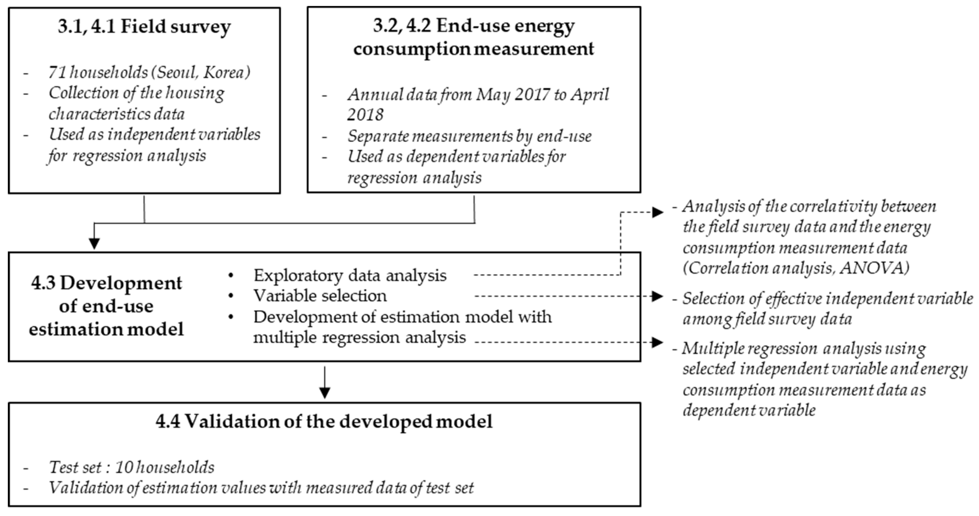
3. Materials and Methods

As shown in Figure 1, information on housing characteristics was collected through a field survey and in-depth interviews with residents of 71 households (15 apartment complexes) in Seoul, South Korea. Annual energy consumption data were collected from measurement systems installed to measure energy consumption by end use. Energy consumption was defined as 7 end uses: heating, cooling, DHW, lighting, ventilation, electric appliances, and cooking. Three energy sources were considered: city gas, electricity, and district heating. The annual end-use energy-consumption data were collected from May 2017 to April 2018. Variables affecting the energy consumption of each end use were identified through correlation analysis and analysis of variance (ANOVA) with SPSS 24. Effective variables for deriving a regression model were selected by repeating multiple regression by end use. Multiple regression analysis was conducted with the selected variables as independent variables, and the measured end-use energy consumption as the dependent variable, and then an end-use energy-consumption estimation model was developed. The regression model developed was validated through a separate test set of 10 households.

3.1. Field Survey Overview

For the 71 households (15 apartment complexes, 4 or 5 units per complex) in Seoul, South Korea, specialized researchers visited each household and collected information on housing characteristics through an in-depth investigation and interviews with residents and apartment managers as shown in Figure 2. The information collected included heat-source type, permit year, area for exclusive use, vertical and horizontal position of the apartment units, orientation, heating, cooling, DHW, lighting, ventilation, electrical- and cooking-equipment-related information (e.g., ownership, number of possessed appliances, usage schedule), and resident information (e.g., age, occupation, gender, and occupancy schedule).

This study also collected weather data (i.e., outdoor temperature and humidity) every hour from the Korea Meteorological Administration. Seoul, the subject area of this research, is located at 37° N latitude, 126° E longitude, and has a temperate climate. These climate zones generally have wider temperature ranges throughout the year, and typically feature 4 distinct seasons: summer is the warmest, winter the coldest, and spring and autumn are mild. Building energy consumption increased in summer and winter due to their severe outdoor conditions. Therefore, this study calculated HDD and CDD based on the collected weather data, and considered their effects for estimating and validating heating and cooling energy consumption. The HDD was calculated to be 2830 °C·day (based on 18.3 °C), and the CDD was calculated to be 186 °C·day (based on 24 °C) for the period between May 2017 and April 2018.

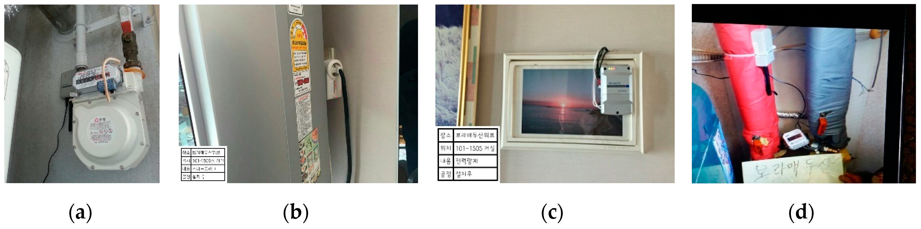
3.2. End-Use Energy-Consumption Classification and Measurement

In general, residential energy consumption is measured according to energy source (e.g., city gas, electricity, and district heating) to impose fees. In this study, energy consumption was classified and defined by end use for analysis of end-use energy consumption. ISO 12655:2013 [14,15] is an international standard for measuring the energy use of buildings that classifies building energy consumption into heating, cooling, DHW, ventilation, lighting, appliance, lift, auxiliary facilities, and so on. As shown in Figure 3, this study classified energy consumption into 7 end-uses: heating, cooling, DHW, lighting, ventilation, electric appliances, and cooking. These were selected in consideration of the energy-consumption proportion of apartments in South Korea based on the classification system of ISO 12655:2013. For heating and DHW, energy consumption was defined as the system main energy source (district heating or city gas) and system-operation energy consumption (electricity). For cooling, the energy consumption of the air conditioner, which is the main cooling equipment, was used (fans were classified as electric appliances). For lighting, the energy consumption of the main lighting equipment, composed of separate branch circuits, was used. For ventilation, the energy consumption of the ventilation unit and exhaust fans in the bathroom and kitchen was used. For electric appliances, the energy consumption of electric devices in the household, such as kitchen appliances (e.g., refrigerator and microwave), household appliances (e.g., washing machine and vacuum cleaner), and information technology devices (IT devices, e.g., computer, printer, etc.) was used. This was calculated by subtracting the energy consumption of heating, cooling, DHW, lighting, ventilation, and the electric cooktop from the total household energy consumption. For cooking, the energy consumption of the main cooking appliances (i.e., gas or electric cooktop) was used.

Measurement systems (e.g., watt-hour meters, smart plugs, calorimeters, and flowmeters) were installed in each household as shown in Figure 4 to measure and calculate energy consumption by end use (detailed process for measurement system installation was referred to [16,17]). Research was conducted on the annual end-use energy-consumption data from May 2017 to April 2018, and data were recorded every hour. All units of the energy consumption measured were converted into kilowatt hours (kWh) to facilitate comparison and analysis of end-use energy consumption.

4. Results

4.1. Field-Survey Results

Based on the housing-characteristics data collected through the field survey and previous studies [4,18,19,20,21], independent variables were classified into buildings, systems, and user-related characteristics, as given in

Table 1. Independent-variable setting.

Category	Variable		Units	Scale	Range
Building-related characteristics	AREA		m2	Ratio	26–137
	PYEAR 1		-	Nominal	(Dummy variable) 0: before 2000, 1: after 2001
	ATYPE		-	Nominal	(Dummy variable) 0: apartment house of staircase type 1: apartment house of corridor access type
	LOCATE_v		-	Nominal	(Dummy variable) (0,0) bottom floor, (1,0) middle floor, (0,1) top floor
	LOCATE_h		-	Nominal	(Dummy variable) 0: on the sides, 1: in the center
	ORIEN		-	Nominal	(Dummy variable) (0,0) southeast or east, (1,0) south, (0,1) southwest or west
	BALCONY		-	Nominal	(Dummy variable) 0: not extended, 1: extended
System-related characteristics	HEAT_temp		°C	Ratio	18–30
	HEAT_sub		-	Nominal	(Dummy variable) 0: not used, 1: used
	HEAT_source		-	Nominal	(Dummy variable) 0: District heating, 1: City gas (individual heating)
	nAIR 2		EA	Ratio	1–3
	AIR_type		-	Nominal	(Dummy variable) 0: stand type, 1: wall type
	AIR_hour 3		-	Nominal	(Dummy variable) (0,0) 2 h or less, (1,0) 12 h or less, (0,1) more than 12 h
	DHW_wm		-	Nominal	(Dummy variable) 0: not used, 1: used
	nDHW		EA	Ratio	3–8
	LD		W/m2	Ratio	2–21
	L_hour		h/day	Ratio	1–12
	LED		-	Ratio	(Dummy variable) 0: not used, 1: used
	V_bath_hour		h/day	Ratio	0.12–3.5
	V_kit_hour		h/day	Ratio	0.12–2
	V_unit		-	Ratio	(Dummy variable) 0: not used, 1: used
	nREF		EA	Ratio	1–5
	nTV		EA	Ratio	1–4
	nPC		EA	Ratio	0–2
	nWP		EA	Ratio	0–1
	nAP		EA	Ratio	0–1
	COOK		-	Nominal	(Dummy variable) 0: electric cooktop, 1: gas cooktop
User-related characteristics	nRES		person	Ratio	1–5
	by gender	nMALE	person	Ratio	0–4
		nFEMALE	person	Ratio	0–4
	by age	nAGE (≥65)	person	Ratio	0–3
		nAGE (20–64)	person	Ratio	0–5
		nAGE (8–19)	person	Ratio	0–3
		nAGE (≤7)	person	Ratio	0–1
	by economic activity 4	nECONO_act	person	Ratio	0–4
		nECONO_inact	person	Ratio	0–4

¹ Permit year is an indicator directly related to the building-envelope insulation performance because it can be estimated from legal regulations on thermal transmittance at the time of the permit year. The permit year of the samples ranged from 1985 to 2007, and South Korean regulations on the thermal transmittance were reinforced stepwise in 2001, 2008, 2010, 2013, and 2015. Thus, permit year was collected in interval scale but was converted into a dummy variable by being set to the nominal scales of before 2000 and after 2001. ² Households with zero cooling energy consumption (households with zero air-conditioners mainly used) were excluded from the samples for developing the estimation model. ³ The average daily air-conditioner operating hours were collected on a ratio scale, but were converted into dummy variables by being set to the nominal scales of 2 h or less, 12 h or less, and more than 12 h to consider frequency distribution, which was created based on the field-survey data. ⁴ Employed individuals 15 years or older with an actual income or unemployed individuals seeking jobs to immediately start working are collectively referred to as economically active people (Statistics Korea, statistical standard terms).

. There are four types of variable: ratio variables and interval variables, which are referred to as quantitative variables (variables that can be measured on numerical values such as weight and area), and nominal variables and ordinal variables, which are referred to as categorical variables (variables that take on a fixed number, assigning each observation to a particular group such as grade, blood type, and gender). For regression analysis, all variables had to be quantitative, so categorical variables were converted into dummy variables, as shown in Table 1. In addition, all sample households were located in the same area (i.e., Seoul); weather data were not used as independent variables.

4.2. End-Use Energy-Consumption Measurement Results

End-use energy consumption measurement results were applied as dependent variables in multiple regression analysis. From the total of 71 households, measurement values without annual data were excluded. To ensure the reliability of the data, it was 10% trimmed: the highest 10% and the lowest 10% of the data were excluded. The selected effective target samples were 42 households for heating, 39 households for cooling, 35 households for DHW, 54 households for lighting, 71 households for ventilation, 39 households for electric appliances, and 37 households for cooking.

Table 2. Annual end-use energy-consumption statistics (unit: kWh/yr).

		Heating	Cooling	DHW	Lighting	Ventilation	Electric Appliances	Cooking
Number of effective samples		42	39	35	54	71	39	37
Average (Ratio)		6926 (51.9%)	117 (0.9%)	1950 (14.6%)	429 (3.2%)	32 (0.2%)	3086 (23.1%)	816 (6.1%)
Max		14,325	292	5184	1147	149	4576	1646
Min		1226	29	386	137	0	2,014	312
Percentile	25th	3506	67	1109	263	14	2,487	530
	50th	6746	105	1693	374	22	3,064	811
	75th	9698	149	2426	581	43	3,586	979
Standard Deviation		3504	68	1111	217	29	641	332

shows the annual end-use energy-consumption statistics, and Figure 5 gives those of the box plot. Heating appeared as the largest proportion in household energy consumption based on annual average consumption, and electric appliances were next: 51.9% for heating, 0.9% for cooling, 14.6% for DHW, 3.2% for lighting, 0.2% for ventilation, 23.1% for electric appliances, and 6.1% for cooking. Because the energy-consumption proportion of ventilation was too low at 0.2%, regression analysis was not applied; instead, a calculation formula was derived based on the information collected on housing characteristics (see Section 4.3.3 for details).

4.3. Development of the End-Use Energy-Consumption Estimation Model

Variables that affect energy consumption were identified through correlation analysis and ANOVA between the information on housing characteristics collected through the field survey and energy-consumption measurement data. The multicollinearity between variables was examined (see Section 4.3.1). Based on this, multiple regression analysis was repeatedly conducted to select the final variables for deriving optimal regression equations by end use (see Section 4.3.2), and an end-use energy-consumption estimation model was derived (see Section 4.3.3).

4.3.1. Exploratory Data Analysis

Because energy consumption is affected by various variables in a complicated manner, the results of statistical analysis between energy consumption and each variable do not have an absolute meaning. This section presents the basic data for selecting the final variables that were required to derive a regression model for estimating end-use energy consumption.

Variables for the ratio scale were examined through correlation analysis. The relationship between each variable and energy consumption was interpreted with a correlation coefficient. This study analyzed that variables had a relationship with energy consumption when the correlation coefficient, as seen in the R column of

Table 3. Correlation analysis for ratio-scale and analysis of variance (ANOVA) for nominal-scale results ^1,2: heating, cooling, and DHW.

Variable			Heating		Cooling		DHW
			R	ANOVA	R	ANOVA	R	ANOVA
			p-R	Cramér	p-R	Cramér	p-R	Cramér
Building	AREA		0.620 *	-	0.177	-	0.264	-
	PYEAR		-	0.072	-	0.290	-	0.065
	ATYPE		-	0.000	-	0.627	-	0.283
				0.780 (AREA)
	LOCATE_v		-	0.012 *	-	0.942	-	0.646
	LOCATE_h		-	0.329	-	0.977	-	0.586
	ORIEN		-	0.527	-	0.188	-	0.322
	BALCONY		-	0.104	-	0.101	-	0.455
System	HEAT_temp		0.538 *	-	n/a	n/a	n/a	n/a
	HEAT_sub		-	0.006 *	n/a	n/a	n/a	n/a
	HEAT_source		-	0.462	n/a	n/a	n/a	n/a
	nAIR		n/a	n/a	0.373 *	-	n/a	n/a
	AIR_type		n/a	n/a	-	0.170	n/a	n/a
	AIR_hour		n/a	n/a	-	0.000 *	n/a	n/a
	DHW_wm		n/a	n/a	n/a	n/a	-	0.225
	nDHW		n/a	n/a	n/a	n/a	0.235	-
User	nRES		0.099	-	0.221	-	0.649 *	-
	By gender	nMALE	0.102	-	0.197	-	0.311	-
							−0.142 (n RES)
		nFEMALE	0.051	-	0.083	-	0.482	-
							0.142 (n RES)
	By age	nAGE(≥65)	−0.106	-	−0.342 *	-	−0.177	-
		nAGE(20–64)	0.114	-	0.241	-	0.516	-
							0.081 (n RES)
		nAGE(8–19)	−0.141	-	0.264	-	0.149	-
		nAGE(≤7)	0.153	-	−0.072	-	0.141	-
	by economicactivity	nECONO_act	0.287	-	0.078	-	0.529	-
							0.129 (n RES)

¹ R: correlation coefficient, p-R: partial correlation coefficients, ANOVA: variable’ p-value in ANOVA. Cramér: Cramér correlation coefficients. ² p-R and Cramér were presented only for multicollinearity occurring. ^* Variables with a relationship with end-use energy consumption.

and

Table 4. Correlation analysis for ratio-scale and AVOVA for nominal-scale results ^1,2: lighting, electric appliances, and cooking.

Variable			Lighting		Electric Appliances		Cooking
			R	ANOVA	R	ANOVA	R	ANOVA
			p-R	Cramér	p-R	Cramér	p-R	Cramér
Building	AREA		0.535 *	-	0.414 *	-	0.123	-
	PYEAR		-	0.017	-	0.299	-	0.798
				0.387 (AREA)
	ATYPE		-	0.007	-	0.033	-	0.548
				0.614 (AREA)		0.630 (AREA)
	LOCATE_v		-	0.283	-	0.677	-	0.733
	LOCATE_h		-	0.889	-	0.601	-	0.498
	ORIEN		-	0.356	-	0.417	-	0.058
	BALCONY		-	0.004	-	0.122	-	0.301
				0.524 (AREA)
System	LD		0.003	-	n/a	n/a	n/a	n/a
	L_hour		0.463 *	-	n/a	n/a	n/a	n/a
	LED		-	0.390	n/a	n/a	n/a	n/a
	nREF		n/a	n/a	0.360 *	-	n/a	n/a
	nTV		n/a	n/a	0.389 *	-	n/a	n/a
	nPC		n/a	n/a	0.272	-	n/a	n/a
	nWP		n/a	n/a	0.294	-	n/a	n/a
	nAP		n/a	n/a	0.183	-	n/a	n/a
	COOK		n/a	n/a	n/a	n/a	-	0.827
User	nRES		0.535 *	-	0.191	-	0.470 *	-
	by gender	nMALE	0.523	-	0.268	-	0.443	-
			0.058 (nRES)				0.185 (nRES)
		nFEMALE	0.321	-	0.027	-	0.092	-
			−0.049 (nRES)
	by age	nAGE(≥65)	−0.178	-	0.180	-	0.037	-
		nAGE(20–64)	0.361	-	−0.019	-	0.169	-
			−0.058 (nRES)
		nAGE(8–19)	0.378 *	-	0.136	-	0.401 *	-
		nAGE(≤7)	−0.186	-	−0.147	-	−0.201	-
	by economic activity	nECONO_act	0.310	-	0.020	-	0.127	-
			−0.310 (nRES)
		nECONO_inact	0.338	-	0.272	-	0.401	-
			0.109 (nRES)				0.291 (nRES)

¹ R: correlation coefficient, p-R: partial correlation coefficients, ANOVA: variable’ p-value in ANOVA. Cramér: Cramér correlation coefficients. ² p-R and Cramér were presented only for multicollinearity occurring. ^* Variables with a relationship with end-use energy consumption.

, was 0.3 or higher; Generally, the correlation coefficient is analyzed that 0.30–0.59 has a correlation, 0.6–0.0.74 has strong correlation, and 0.75 or higher has very strong correlation [22], and this study found that most of the variables with a correlation coefficient of 0.3 or higher presented as significant in regression analysis. In addition, the correlation coefficient between variables was examined for checking multicollinearity. If correlation between variables was observed, partial correlation analysis was conducted with setting the other as the control variable. Partial correlation coefficients were calculated for the variables with a correlation coefficient of 0.3 or higher, and Table 3 and Table 4 gave partial correlation coefficients, which was written in the p-R column, and corresponding control variable.

Variables for the nominal scale were examined through ANOVA. The statistical significance of the average energy-consumption difference between groups was verified with ANOVA. This study interpreted that variables indicated a relationship with energy consumption when an ANOVA p-value (significance probability), which is in the ANOVA column of Table 3 and Table 4, was 0.05 or lower (significance level, 5%). To examine multicollinearity, Cramér correlation coefficients between variables were calculated, and this study found that variables with a 0.3 or higher coefficient had a relationship. Cramér correlation coefficients were calculated for the variables with ANOVA p-value of 0.05 or lower, and Table 3 and Table 4 gave Cramér correlation coefficients, which is in the Cramér column, and the corresponding variable.

Table 3 and Table 4 present exploratory data analysis results for six end uses: heating, cooling, DHW, lighting, electric appliances, and cooking. For ventilation, statistical values were investigated for deriving the calculation formula: average bathroom ventilation fan power was 30 W, average kitchen exhaust fan power was 90 W, and annual average energy consumption of ventilation unit was 25 kWh/yr.

(1) Heating

AREA (area for exclusive use), LOCATE_v (apartment-unit vertical location), HEAT_temp (heating setting temperature), and HEAT_sub (use of auxiliary heating equipment) indicated a relationship with energy consumption. Although all building-related variables theoretically affect heat loss and heat gain, only AREA and LOCATE_v were found to be significant for heating. AREA showed a strong correlation with heating energy consumption at a correlation coefficient of 0.620. LOCATE_v exhibited a p-value of 0.012, which indicates that the average difference between heating energy consumption of the bottom, middle, and top floors was significant. In case of ATYPE, the average difference of heating energy consumption according to access type could be significant with an ANOVA p-value of 0.000. However, the Cramér correlation coefficient between ATYPE and AREA was 0.780; this is because apartment units with a large area are distributed more to the staircase type. Thus, ATYPE could not be an effective variable for heating energy consumption because there was multicollinearity between AREA and ATYPE. Among system-related variables, HEAT_temp and HEAT_sub were found to be significant. HEAT_temp was strongly correlated with heating energy consumption at a correlation coefficient of 0.538. HEAT_sub exhibited a p-value of 0.006, which indicated that the average difference in heating energy consumption according to the status of auxiliary heating-equipment use (e.g., electric heaters and electric heating pads) was significant. User-related variables did not exhibit significant correlations when residents were classified by gender, age, and economic activity. However, nECONO_act exhibited weak positive correlation at a correlation coefficient of 0.287, which means that the more economically active people are, the more heating energy consumption is likely to appear.

(2) Cooling

The nAIR (number of air-conditioners mainly used), AIR_hour (average daily air-conditioner operating hours), and nAGE (≥65, number of residents aged 65 or older) indicated a relationship with energy consumption. None of the building-related variables had a significant relationship with energy consumption. The correlation coefficient of nAIR was 0.373, which indicates that cooling energy consumption increased with the number of air conditioners. The p-value of AIR_hour was 0.000, which indicated that the average difference in cooling energy consumption in average daily air-conditioner operating hours (i.e., 2 h or less, 12 h or less, and more than 12 h) was significant. The correlation coefficient of nAGE (≥65) was higher than ±0.3, which indicates that cooling energy consumption decreased as the number of elderly people (aged 65 or older) increased.

(3) DHW

Only nRES (number of residents) exhibited a relationship with energy consumption, with a correlation coefficient of 0.649. No significant relationship was observed with other building-related and system-related variables. From gender, age, and economic-activity variables, nMALE, nFEMALE, nAGE (20–64), and nECONO_act were correlated with DHW energy consumption. However, when partial correlation analysis was conducted with nRES as the control variable, none of gender, age, or economic activity exhibited significant relation.

(4) Lighting

The AREA (area for exclusive use), L_hour (average daily lighting hours), nRES (number of residents), and nAGE (8–19, number of residents aged between 8 and 19) indicated a relationship with energy consumption. Only AREA exhibited correlation among building-related variables, with a correlation coefficient of 0.535. The ANOVA p-value was less than 0.05 for PYEAR, ATYPE, and BALCONY, but the Cramér coefficient with AREA was greater than 0.3, which indicates that these variables had a correlation with AREA. In other words, the difference was not caused by permit year, access type, and balcony-extension status, but rather by the fact that the area for exclusive use distribution was not uniform in the groups. Of the system-related variables, the correlation coefficient of L_hour was 0.463, which indicates positive correlation. Of the user-related variables, the correlation coefficient of nRES and nAGE (8–19) was 0.535 and 0.378, respectively, which indicate positive correlation. The nMALE, nFEMALE, nAGE(20–64), nECONO_act variables did not had a significant relationship with lighting energy consumption according to partial correlation analysis with nRES as a control variable.

(5) Electric appliances

AREA, nREF (number of refrigerators, including kimchi refrigerator), nTV (Number of TVs) indicated a relationship with energy consumption. AREA, nREF, and nTV exhibited a relationship with a correlation coefficient of 0.414, 0.360, and 0.389, respectively. nWP had a weak positive relationship with a correlation coefficient of 0.294, which was approximated to 0.3. From user-related variables, no variable exhibited a significant relationship with a correlation coefficient of 0.3 or higher.

(6) Cooking

nRES and nAGE indicated a relationship with energy consumption. None of the building-related and system-related variables exhibited a significant relationship. From user-related variables, nRES and nAGE were correlated with cooking energy consumption at a correlation coefficient of 0.470, 0.401 each. It was inferred that the more residents there were, the higher cooking energy consumption was; students (aged between 8 and 19) played an especially key role in cooking energy consumption. nECONO_inact was correlated with cooking energy consumption, but when partial correlation analysis was conducted with nRES as a control variable, it showed weak positive correlation, at a partial correlation coefficient of 0.291.

4.3.2. Variable Selection

Methods for selecting variables in multiple regression analysis are largely divided into forward, backward, and stepwise selection. Forward selection adds variables one by one in the order of the highest p-value. In contrast, backward selection deletes variables one by one in the order of the lowest p-value after all variables are entered. In stepwise selection, forward and backward selection are alternated; this is the most commonly used variable-selection method. This study conducted variable selection by hand, not by SPSS, using the stepwise selection approach for all variables in Table 1 to consider a relationship between variables and energy consumption, the importance of each variable, and so on, as well as the variable p-values. Addition and deletion of variables were repeated based on the correlation with end-use energy consumption or in the order of the highest p-value. The relationship with energy consumption can be found in the results of Section 4.3.1.

4.3.3. Development of Estimation Model with Multiple Regression Analysis

The final variables selected were used as independent variables, and end-use energy-consumption measurement data were used as dependent variables. A regression model for estimating end-use energy consumption (kWh/yr) was developed through multiple regression analysis, as shown in Equations (1)–(7), excluding Equation (5). Regression analysis was not performed for ventilation energy consumption because its proportion of the total energy consumption was extremely low. Instead, a calculation formula was derived using ventilation-fan power and operation hours based on the collected information on housing characteristics. In Section 4.3.1, the average bathroom ventilation fan power was 30 W, average kitchen exhaust-fan power was 90 W, and the annual average energy consumption of ventilation units was 25 kWh/yr. Equation (5) shows the calculation formula for estimating ventilation energy consumption.

Table 5. Regression analysis results of the estimation model.

-	Heating	Cooling	DHW	Lighting	Ventilation	Electric Appliances	Cooking
Equation	(1)	(2)	(3)	(4)	(5)	(6)	(7)
Adj-R2	0.643	0.703	0.406	0.548	-	0.407	0.429
F-ratio (p-value)	15.767 (0.000)	18.996 (0.000)	12.631 (0.000)	11.694 (0.000)	-	5.355 (0.001)	6.000 (0.001)

presents Adj-R², F-ratio, and the p-value of the regression model for estimating end-use energy consumption. All regression models were statistically valid at a p-value of 0.05 or less. Adj-R² was exhibited from 0.406–0.703, which means that the explanation power of the model is 40.6%–70.3%.

$$\begin{array}{l}{\mathrm{E}}_{\mathrm{Heating}}\\ =-10,686.1+68.6\times AREA-5,521.1\times LOCATE\_v\left(dummy1\right)-1,122.4\times LOCATE\_v\left(dummy2\right)\\ -1,434.2\times LOCATE\_h+782.5\times HEAT\_temp\end{array}$$

(1)

$$\begin{array}{l}{\mathrm{E}}_{\mathrm{Cooling}}\\ =-19.8+1.3\times AREA+46.9\times AIR\_hour\left(dummy1\right)+294.4\times AIR\_hour\left(dummy2\right)\\ -36.9\times nAGE\left(\ge 65\right)+13.9\times nAGE\left(8-19\right)\end{array}$$

(2)

$${\mathrm{E}}_{\mathrm{DHW}}=-407.7+5.2\times AREA+646.4\times nRES$$

(3)

$$\begin{array}{l}{\mathrm{E}}_{\mathrm{Lighting}}\\ =-73.6+2.9\times AREA+103.6\times BALCONY+24.4\times L\_hour+15.4\times nAGE\left(\ge 65\right)\\ +34.9\times nAGE\left(20-64\right)+125.9\times nAGE(8-19)\end{array}$$

(4)

$${\mathrm{E}}_{\mathrm{Ventilation}}=\left(30\times V\_bath\_hour+90\times V\_kit\_hour\right)\times 0.365+25\times V\_unit$$

(5)

$$\begin{array}{l}{\mathrm{E}}_{\mathrm{Electric}\mathrm{appliances}}\\ =185.9+6.7\times AREA+407.3\times nREF+334.1\times nTV+605.7\times nWP+101.9\times nECONO\_act\\ +373.8\times nECONO\_inact\end{array}$$

(6)

$$\begin{array}{l}{\mathrm{E}}_{\mathrm{Cooking}}\\ =-232.3+259.4\times nAGE\left(\ge 65\right)+175.3\times nAGE\left(20-64\right)+374.6\times nAGE\left(8-19\right)\\ +440.2\times COOK\end{array}$$

(7)

4.4. Validation of End-Use Energy-Consumption Estimation Model

The regression models derived were validated using measurement data of the test set. Ten apartment units from the training set, which had annual data for another measurement period, were selected for test set; it was difficult to make training and test sets for the same period due to the limited number of samples. Thus, the test set was formed by selecting samples that had complete annual data for the different measurement period from the training set. The measurement period of the test set was from June 2016 to May 2017, and for the training set was from May 2017 to April 2018. Because test and training sets had different measurement periods, the average difference between the two sets was verified through a paired T-test, as given in

Table 6. Paired T-test results for 10 households’ measurement data of test and training sets.

	Heating 1	Cooling	DHW	Lighting	Ventilation	Electric Appliances	Cooking
p-value	0.011	0.506	0.575	0.475	0.521	0.473	0.566

¹ Test set average heating energy consumption: 5644 kWh/yr. Training set average heating energy consumption: 6590 kWh/yr.

. If the p-value was lower than 0.05, it indicated that the average difference between the two groups was statistically significant at a significance level of 5%. In Figure 6, we can see that the heating energy consumption of most households in the test set was lower than that of the training set, but cooling energy consumption did not show specific patterns (the rest was the same as cooling).

For all end uses except for heating, the average difference between the test and training sets was statistically insignificant. For heating, the p-value was 0.011, which indicates that the average difference (=946, 6590–5644 kWh/yr) between the two groups was valid. The weather data for the measurement period of test and training set are as follows. It can be inferred that there was no noteworthy difference in energy consumption except for heating in spite of climate-condition differences. In addition, we can conclude that the average difference of heating energy consumption between the test and training set comes from the HDD difference.

• Test-set weather data: June 2016 to May 2017
  • HDD (based on 18.3°C): 2624 °C·day
  • CDD (based on 24.0°C): 236 °C·day
  • Average solar radiation: 149 Wh/m²
• Training-set weather data: May 2017 to April 2018
  • HDD (based on 18.3°C): 2830 °C·day
  • CDD (based on 24.0°C): 186 °C·day
  • Average solar radiation: 142 Wh/m²

Because the average difference of heating energy consumption (=946 kWh/yr) is statistically valid, the estimated heating energy consumption of the test set was calculated by subtracting 946 kWh from the results with Equation (1). For the other end uses, the estimated values were calculated with Equations (2)–(7). Measured and estimated consumption, and error by end use, are given in

Table 7. Validation of the estimation model with measured data.

End-use		Validation for 10 Households
		1	2	3	4	5	6	7	8	9	10
Heating	Measured (kWh/yr)	7008	5407	14,044	8955	6955	4674	2624	7839	5805	4349
	Estimated (kWh/yr)	5937	5296	12,022	6753	7529	6891	3136	6993	8773	4620
	Error (%)	−18	−2	−17	−33	8	32	16	−12	34	6
Cooling	Measured (kWh/yr)	274	78	52	80	236	183	32	157	139	77
	Estimated (kWh/yr)	308	89	49	77	246	221	24	154	149	90
	Error (%)	11	13	−9	−4	4	17	−31	−2	7	14
DHW	Measured (kWh/yr)	1811	1296	1296	2743	3806	2228	1981	3274	1148	892
	Estimated (kWh/yr)	1432	1153	1397	2024	4021	2876	1909	3567	1216	686
	Error (%)	−26	−12	7	−35	5	23	−4	8	6	−30
Lighting	Measured (kWh/yr)	576	302	247	698	520	262	241	510	456	311
	Estimated (kWh/yr)	633	301	278	726	531	282	222	565	425	333
	Error (%)	9	0	11	4	2	7	−8	10	−7	6
Ventilation	Measured (kWh/yr)	50	46	57	85	38	21	18	38	38	13
	Estimated (kWh/yr)	54	38	100	97	38	27	20	45	38	21
	Error (%)	6	−22	42	13	0	0	13	16	0	36
Electric Appliance	Measured (kWh/yr)	3782	3329	2361	4189	3282	2333	2647	2995	2662	3523
	Estimated (kWh/yr)	3995	3418	2427	4455	3352	2568	2980	2687	3019	3428
	Error (%)	5	3	3	6	2	9	11	−11	12	−3
Cooking	Measured (kWh/yr)	773	1029	795	969	1463	879	879	879	757	735
	Estimated (kWh/yr)	737	963	762	991	1508	975	922	1037	705	735
	Error (%)	−5	−7	−4	2	3	10	5	15	−19	6

. The maximum error between the measured and estimated values was around ±30%.

5. Discussion

Many previous studies have utilized weather-data-related variables (e.g., HDD, CDD) for estimating heating and cooling energy consumption. Fumo and Biswas [8] analyzed various residential energy-consumption prediction methodologies using regression analysis (e.g., linear and nonlinear regression), and then suggested simple and multiple regression models for electricity consumption in June 2013. They used dry-bulb temperature as an independent variable, and the regression coefficient was positive, which means that cooling energy consumption increases as outdoor temperature increases. In addition, Li [9] also used sqrtCDD65 as an independent variable for a cooling estimation model. However, in Section 4.4, actual measurement data showed that cooling energy consumption was rarely affected by weather data, while heating energy consumption decreased as HDD decreased. Related to this, follow-up research is needed with more samples over a longer period to present meaningful data.

The Adj-R² of the regression model for estimating end-use energy consumption was in the order of cooling (0.703) > heating (0.643) > lighting (0.548) > cooking (0.429) > electric appliances (0.407) > DHW (0.406), and a higher Adj-R² indicates that the regression model had a higher explanatory power for the samples. For cooking, electric appliances, and DHW, where Adj-R² was mediocre at the level of 0.4, further studies on variables capable of increasing the explanatory power or other statistical approaches are needed. Aydinalp-Koksal and Ugursal [4] developed a space heating, DHW and appliance, lighting, and cooling (ALC) estimation model using the neural-network, CDA, and engineering methods, and they applied the following variables: owner or rent status, household income, number of adults, number of children for DHW, refrigerators, secondary refrigerators, dishwashers, clothes dryers, and minor electric appliances. In this study, Adj-R² appeared as 0.795 for ALC, 0.814 for DHW, and 0.892 for space heating (with the CDA approach). On the other hand, Matsumoto [10] applied CDA methodology for estimating electric-appliance energy consumption. He utilized not only appliance ownership but also household income as independent variables, and divided appliances into old and new ones. However, Adj-R² appeared to be only between 0.400 and 0.428. Newsham and Donnelly [19] also use CDA approach and divided appliances into old one ( >10 years) and new one ( <10 years), and Adj-R² appeared to be 0.525 for electrical appliances, 0.792 for natural gas appliances.

6. Conclusions

The purpose of this study was to develop an estimation model for end-use energy consumption in the residential sector. In this study, information on housing characteristics was collected through a field survey of 71 households in Seoul, South Korea, and annual energy consumption by end use was collected from May 2017 to April 2018 from installed measurement systems. Based on the data collected, the relationship between end-use energy consumption and housing characteristics was analyzed by correlation analysis and ANOVA. Multicollinearity between variables was also analyzed. A correlation coefficient of 0.3 or higher was interpreted as significant in correlation analysis, and a p-value at the 5% level (0.05 or lower) was interpreted as significant in ANOVA. Significant variables were found to be AREA, LOCATE_v, HEAT_temp, and HEAT_sub for heating; nAIR, AIR_hour, and nAGE (≥65) for cooling; nRES (Number of residents) for DHW; AREA, L_hour, nRES, and nAGE (8–19) for lighting; AREA, nREF, nTV for electric appliances; and nRES and nAGE (8–19,) for cooking. For most end uses, AREA, nAGE (8–19), and nAGE (≥65) exhibited crucial variables.

The final variables by end use were selected using repeated multiple regression analysis with the stepwise selection method. The estimation model for end-use energy consumption was derived from where selected final variables were used as independent variables, and energy-consumption measurement data were used as dependent variables. For ventilation, a calculation formula was derived instead of a regression equation because its proportion of total energy consumption was very low. The Adj-R² of the estimation model ranged from 0.406 to 0.703 depending on end use. The end-use energy-consumption estimation model was validated with a separate test set (10 households), and the maximum error between the measured and estimated values was around ±30%. The error rates of heating, cooling, and DHW, which are affected by climate conditions, were especially greater compared to the error of lighting, ventilation, electric appliances, and cooking, with relatively less fluctuation in energy consumption throughout the year. However, in-depth analysis of the error between measured and estimated was difficult because of the limited number of samples. A follow-up study with more samples and related researches [23,24,25] is required to analyze the household characteristics that have a higher error and to improve the estimation models. In addition, the heating estimation model of this study was limited to Seoul, South Korea (HDD based on 18.3 °C: 2830 °C·day).

References

1. Korea Energy Economics Institute; Korea Energy Agency. 2017 Energy Consumption Survey; Ministry of Trade, Industry and Energy: Sejong, Korea, 2018.
2. Swan, L.G.; Ugursal, V.I. Modeling of end-use energy consumption in the residential sector: A review of modeling techniques. Renew. Sustain. Energy Rev. 2009, 13, 1819–1835. [Google Scholar] [CrossRef]
3. Shimoda, Y.; Fujii, T.; Morikawa, T.; Mizuno, M. Development of residential energy end-use simulation model at city scale. In Proceedings of the Eighth International IBPSA Conference, Eindhoven, The Netherlands, 11–14 August 2003; pp. 1201–1208. [Google Scholar]
4. Aydinalp-Koksal, M.; Ugursal, V.I. Comparison of neural network, conditional demand analysis, and engineering approaches for modeling end-use energy consumption in the residential sector. Appl. Energy 2008, 85, 271–296. [Google Scholar] [CrossRef]
5. Ryan, P.; Pavia, M. Australian residential energy end-use—Trends and projections to 2030. In Proceedings of the 2016 ACEEE Summer Study on Energy Efficiency in Buildings, Pacific Grove, CA, USA, 21–26 August 2016. [Google Scholar]
6. Ren, Z.; Foliente, G.; Chan, W.Y.; Chen, D.; Ambrose, M.; Paevere, P. A model for predicting household end-use energy consumption and greenhouse gas emissions in Australia. Int. J. Sustain. Build. Technol. Urban Dev. 2013, 4, 210–228. [Google Scholar] [CrossRef] [Green Version]
7. Min, J.; Hausfather, Z.; Lin, Q.F. A high-resolution statistical model of residential energy end use characteristics for the United States. J. Ind. Ecol. 2010, 14, 791–807. [Google Scholar] [CrossRef]
8. Fumo, N.; Biswas, M.A.R. Regression analysis for prediction of residential energy consumption. Renew. Sustain. Energy Rev. 2015, 47, 332–343. [Google Scholar] [CrossRef]
9. Li, C. Home Energy Consumption Estimation by End Use and Energy Efficiency Upgrade Recommendations. Master’s Thesis, Nicholas School of the Environment, Duke University, Durham, NC, USA, 2014. [Google Scholar]
10. Matsumoto, S. Electric Appliance Ownership and Usage: Application of Conditional Demand Analysis to Japanese Household Data; Working Paper E-98; Tokyo Center for Economic Research: Tokyo, Japan, 2015. [Google Scholar]
11. Parti, M.; Parti, C. The total and appliance-specific conditional demand for electricity in the household sector. Bell J. Econ. 1980, 11, 3029–3321. [Google Scholar] [CrossRef]
12. Larsen, B.M.; Nesbakken, R. Household electricity end-use consumption: Results from econometric and engineering models. Energy Econ. 2004, 26, 179–200. [Google Scholar] [CrossRef]
13. Aydinalp-Koksal, M.; Ugursal, V.I.; Fung, A.S. Modeling of the appliance, lighting, and space-cooling energy consumption in the residential sector using neural network. Appl. Energy 2002, 71, 87–110. [Google Scholar] [CrossRef]
14. ISO 12655:2013. Energy Performance of Buildings: Presentation of Measured Energy Use of Buildings; International Organization for Standardization: Geneva, Switzerland, 2013. [Google Scholar]
15. ISO 16346:2013. Energy Performance of Buildings: Assessment of All Overall Energy Performance; International Organization for Standardization: Geneva, Switzerland, 2013. [Google Scholar]
16. Choi, B.; Jin, H.; Kang, J.; Kim, S.; Lim, J.; Song, S. Measurement and normalization methods of energy consumption by end-use in apartment buildings for providing detailed energy information. J. Korean Inst. Archit. Sustain. Environ. Build. Syst. 2015, 9, 437–447. [Google Scholar]
17. Kang, J.; Kim, S.; Jin, H.; Lim, S.; Lim, J.; Song, S. Development of estimation model for end-use energy consumption by usage in apartment building units via conditional demand analysis. J. Korean Inst. Archit. Sustain. Environ. Build. Syst. 2017, 11, 131–141. [Google Scholar]
18. Chen, J.; Wang, X.; Steemers, K. A statistical analysis of a residential energy consumption survey study in Hangzhou, China. Energy Build. 2013, 66, 193–202. [Google Scholar] [CrossRef]
19. Newsham, G.R.; Donnelly, C.L. A model of residential energy end-use in Canada: Using conditional demand analysis to suggest policy options for community energy planners. Energy Policy 2013, 59, 133–142. [Google Scholar] [CrossRef] [Green Version]
20. Lee, K.; Yang, J.; Ryu, U. A study on the estimation model of the amount of the electric energy consumption according to the apartment heating type. J. Korea Inst. Ecol. Archit. Environ. 2010, 10, 57–64. [Google Scholar]
21. Bedir, M.; Hasselaar, E.; Itard, L. Determinants of electricity consumption in Dutch dwelling. Energy Build. 2013, 58, 194–207. [Google Scholar] [CrossRef]
22. Rea, L.M.; Parker, R.A. Designing and Conducting Survey Research: A Comprehensive Guide, 3rd ed.; Jossey-Bass: San Francisco, CA, USA, 2005; ISBN 978-0787975463. [Google Scholar]
23. Ruiz, G.R.; Bandera, C.F. Validation of calibrated energy models: Common errors. Energies 2017, 10, 1587. [Google Scholar] [CrossRef]
24. Katipamula, S.; Brambley, M.R. Methods for Fault Detection, Diagnostics, and Prognostics for Building Systems—A Review, Part II. HVAC R Res. 2005, 11, 169–187. [Google Scholar] [CrossRef]
25. Deshmukh, S.; Glicksman, L.; Norford, L. Case study results: Fault detection in air-handling units in buildings. Adv. Build. Energy Res. 2018, 1756–2201. [Google Scholar] [CrossRef]
Figure 1. Research flowchart for the development of the regression model.
Energies 12 02327 g001
Figure 2. Housing-characteristics data collection through a field survey.
Energies 12 02327 g002
Figure 3. End-use energy-consumption classification and definitions.
Energies 12 02327 g003
Figure 4. Energy-consumption measurement-system installation: (a) gas flowmeter for heating and domestic hot water (DHW), (b) watt-hour meter for cooling, (c) watt-hour meter for total household power, and (d) hot-water calorimeter for DHW.
Energies 12 02327 g004
Figure 5. Annual energy consumption by end use.
Energies 12 02327 g005
Figure 6. Ten households’ measurement data of test and training sets: (a) heating (b) cooling.
Energies 12 02327 g006