Short-Term Wind Speed Prediction Based on Variational Mode Decomposition and Linear–Nonlinear Combination Optimization Model

Abstract

Wind power, one of renewable energy resources, is a fluctuating source of energy that prevents its further participation in the power market. To improve the stability of the wind power injected into the power grid, a short-term wind speed predicting model is proposed in this work, named VMD-P-(ARIMA, BP)-PSOLSSVM. In this model, variational mode decomposition (VMD) is combined with phase space reconstruction (P) as data processing method to determine intrinsic mode function (IMF) and its input–output matrix in the prediction model. Then, the linear model autoregressive integrated moving average model (ARIMA) and typical nonlinear model back propagation neural network (BP) are adopted to forecast each IMF separately and get the prediction of short-term wind speed by adding up the IMFs. In the final stage, particle swarm optimization least squares support vector machine (PSOLSSVM) uses the prediction results of the two separate models from previous step for the secondary prediction. For the proposed method, the PSOLSSVM employs different mathematical principles from ARIMA and BP separately, which overcome the shortcoming of using just single models. The proposed combined optimization model has been applied to two datasets with large fluctuations from a northern China wind farm to evaluate the performance. A performance comparison is conducted by comparing the error from the proposed method to six other models using single prediction techniques. The comparison result indicates the proposed combined optimization model can deliver more accurate and robust prediction than the other models; meanwhile, it means the power grid dispatching work can benefit from implementing the proposed predicting model in the system.

1. Introduction

With the continuous reduction of traditional fossil energy and the salient environmental pollution problem, the global energy crisis is becoming more and more serious. From the dual demand of human society for energy and environmental protection, renewable energy is bound to become the direction of future energy due to its advantages of being clean, pollution-free, and recyclable. As a sort of renewable energy, wind energy has the advantages of wide source and convenient development, but it also exhibits strong volatility, intermittent, and non-control characteristics, which pose great challenges to the safety and stability of grid system. Accurate and reliable short-term wind speed prediction not only minimizes the economic losses caused by wind power grid connection, but also reduces the risk of grid dispatch and grid transmission [1].

Considering the development of the wind speed prediction method, the principle gradually changes from the physical method to the statistical, and the prediction method is developed from linear prediction to nonlinear. In recent years, the intelligent algorithm has been adopted and optimized gradually. Wanting to improve the accuracy of prediction and make up for the shortcomings of separate methods, more and more scholars have explored combined prediction methods. In summary, the wind speed prediction methods can be roughly divided into five categories: (a) Physical methods, (b) spatial correlation, (c) conventional statistical methods, (d) artificial intelligence algorithms, (e) combined methods.

The input indexes of the physical methods are geographical information of the wind farm such as meteorological message, topographical features, surface roughness, obstacles, etc. [2], then analyzing and calculating the input comprehensively can obtain the wind speed and direction of the fan hub height [3]. Physical methods regard NWP (numerical weather prediction system) as the chief technology, which has excellent performance in medium- and long-term wind speed prediction [4], but NWP has some disadvantages including complex calculation, time-consuming, and high accuracy requirements for basic physical quantities [5]. The position of the spatial correlation methods in the wind speed prediction field has been raised to the same height as physical methods and statistical methods since 2014 [6]. Spatial correlation believes that the wind speed of a certain place has a high correlation with the wind speed of neighborhood spaces, making it possible to use the weather and other information of the surrounding areas to improve the local wind speed prediction effect [7]. The key in spatial correlation prediction is establishing mapping relationship through the regression analysis method, so the optimizations of the method mean all of it.

The statistical models predict future wind speed by analyzing historical statistics [8]. Conventional statistical methods include AR (autoregressive) model [9], ARMA (autoregressive moving average) model [10], ARIMA (autoregressive integral moving average) model [11], and SARIMA (seasonal autoregressive integral moving average) model [12]. The most notable method is the ARIMA method proposed by Box-Jenkins [13], which has the advantages of a simple principle and high precision. Because ARIMA can effectively extract linear features of data [14] and improve the adaptability of time-series models [15], it performed well in wind speed prediction. Torres et al. [16] compared the ARIMA with the persistence model and found that the ARIMA always performed better in the prediction. The deformation of the ARIMA model has also been widely used already. Liu et al. [17] used ARIMA to determine the parameters of the KF (Kalman Filter) to optimize the model and improve the performance. Based on the ARIMA model, Erdem et al. [18] presented four prediction methods: Component ARMA, link AMRA, VAR (vector autoregressive), and restricted VAR, and applied them to forecast wind speed and direction of two wind farms in North Dakota, USA.

Yuan et al. [19] confirmed that wind speed has obvious chaotic fractal characteristics by using chaos theory, which means wind speed is nonlinear to some extent. Therefore, using the model with a strong ability to extract the nonlinear information can predict the wind speed accurately; meanwhile, the machine model is generally considered to display complex nonlinear relationships well because of its strong robustness and fault tolerance to noise. According to these, a lot of studies have verified that machine models have good pertinence and adaptability to wind speed prediction. In order to interconnect the chaos theory and machine model, Sun et al. [20] performed phase space reconstruction on the decomposed wind speed to determine the input and output matrix of BP. Nowadays, artificial intelligence techniques for predicting wind speed are divided into two categories according to different principles: ANN (artificial neural networks) and SVM (support vector machines). ANN mainly covers BP [21], ELM (extreme learning machines) [22], RBF (radial basis function neural networks) [23], RNN (recurrent neural networks) [24], and so on. As the main representative of ANN, BP has strong nonlinear mapping ability and is used in wind speed prediction widespread research. Qu et al. [25] optimized BP with FPA (flower-pollination algorithm) to predict the wind speed components and obtain excellent results. Yang et al. [26] combined Broyden family with wind driven optimization to determine initial weights and thresholds of BP, and the result proved that optimization increase the prediction precision and reliability effectively. The core of SVM is kernel function which avoids selecting the structure of neural network and handles local minimum points of BP. Kernel function and penalty factor are two important parameters of SVM, so many optimization algorithms are combined with the SVN to select the best parameters, such as cuckoo search algorithm [27] and improved chicken algorithm [28]. The PSO (particle swarm optimization) combined with LSSVM (least squares support vector machine) was proved have advantages of short training time and high precision according to the research of Zhang et al. [29].

Intending to extract effective information from wind speed series, the original signal is usually decomposed into stable sequences in the widespread wind speed prediction researche [30]. Existing decomposition techniques mainly contains WD (wavelet decomposition) and EMD (empirical mode decomposition). Liu et al. [31] proposed three hybrid models based on WD for wind speed prediction, which regard wavelet and wavelet packet as decomposition algorithms. Hu et al. [32] applied the data processed by WD to LSSVM for single-step and multi-step wind speed prediction. Additionally, Liu H et al. [33] used FEEMD (fast ensemble empirical mode decomposition) to process wind speed and established the FEEMD-MEA-MLP model to demonstrate its excellent effect. Wang et al. [22] put forward a hybrid model that amalgamates EMD with Elman neural network for wind speed prediction and confirmed that the proposed method has the smallest MAE (mean absolute error), RMSE (root mean square error), and MAPE (mean absolute proportional error) among the compared models. However, WD has to set the mother wavelet function artificially, while EMD exists as some intractable problems such as lacking mathematical theory, interpolation selection, and modal aliasing phenomenon [34]. In contrast, the VMD method proposed by Konstantin Dragomiretskiy [35] in 2014 not only overcomes the mode mixing, but also decomposes components of different frequencies adaptively. Both Ali Akbar Abdoos [36] and Ali M [37] have proved the outstanding performance of VMD in the wind speed data processing.

Correlation study of Bates et al. [38] evidenced the combined prediction is capable of breaking the limitations of separate prediction models, absorbing the advantages of two or more methods, and reducing the difficulty of model selection, thus, the results of combined prediction tend to be more accurate. According to the combination mode of separate models, it is usually to divide the combined model into series and parallel methods. The series method is making the second prediction of the first results or error correction of first residual by regarding the result or residual as the input of another model, such as [39] and [40]. Similarly, the parallel method uses several models to predict original data separately and then weight the results of the separate prediction models by other methods to form the combination prediction results such as [41] and [42]. Furthermore, more studies combine different signal decomposition techniques into predictions and various optimization algorithms. For example, Liu et al. [43] employed WPD (wavelet packet decomposition) and EMD to decompose the wind speed in turn to make the sequences more stable and then use ELM to make the prediction. Jiang et al. [44] combined BA (bat algorithm), FA (firefly algorithm), and CS (cuckoo search) to optimize the weight coefficients of the three neural networks in order to obtain higher prediction accuracy.

On account of the superiority of the parallel combination and the features of the wind speed being linear accompanied with chaotic, this study put forward a new combined prediction optimization model named VMD-P-(ARIMA, BP)-PSOLSSVM to forecast the wind speed in the short term. The novel model combines the emerging signal decomposition technology, chaos theory, with linear and nonlinear prediction technology to make contributions as follow: (a) Intending to collect the usable information from the original wind speed, a signal processing method based on VMD and phase space reconstruction is invented for the first time. Firstly, the raw data is decomposed into several stable sequences by using VMD, which has been newly proposed in recent years. Then, phase space reconstruction method based on the chaos principle is used to determine the input and output matrix of the prediction model to upgrade the prediction ability. (b) In order to express the strength of the separate models, the research adopts a parallel way to combine the typical linear prediction model and ANN model. Specifically, the processed components and residuals are predicted by ARIMA and BP, respectively, to obtain the predicted values by summing the IMFs. (c) In this study, two results predicted by ARIMA and BP in parallel are used as the input of the LSSVM optimized by PSO for the secondary prediction to obtain the final combined result. PSOLSSVM is a completely different model from the ARIMA and BP from the principle aspect and using this model to make secondary prediction can overcome the limitations of separate models. (d) The excellent performance of the new combined model is evaluated by comparing the prediction results to six other models. Moreover, another set of data was collected to repeat the same experiment and the result confirmed the versatility and application of the proposed model.

The schedule of the paper is showed as follow: Section 2 presents the rationales of VMD, phase space reconstruction, ARIMA, BP, and PSOLSSVM; the construction process of the combination model is given in Section 3; Section 4 uses the proposed model to predict the wind speed in the short term; Section 5 analyzes and discusses the results of Section 4; Section 6 demonstrates the repeatability of the experiment with different cases; Section 7 draws conclusions from two experiments.

2. Materials and Methods

2.1. Variational Mode Decomposition

As a novel non-recursive decomposition method based on the variational problem, VMD decompose nonlinear or non-stationary signals excellently. Compared with WD and EMD, VMD can not only determine the relevant band adaptively, but also avoid the modal aliasing phenomenon, which, because of VMD, has complete and rigorous mathematical theory system and balances the error between modes properly [45]. The existence of the variational problem is getting the bandwidth of each mode and specific construction process is expressed as: (a) Hilbert transform calculates the correlation analysis signal to obtain the unilateral spectrum. (b) Unilateral spectrum should be exponential, tuned to the corresponding estimated center frequency, and moved to the “baseband”. (c) Estimate the bandwidth by demodulating the Gaussian smoothness of the signal. The constrained variational problem established as follows:

$$\begin{gathered} \underset{\left\{u_k\right\},\left\{{\omega }_k\right\}}{min}\left\{{\displaystyle \sum }_k\parallel {\partial }_t\left[\left(\delta \left(t\right)+\frac{j}{\pi t}\right)\ast u_k\left(t\right)\right]{e^{-j{\omega }_{k}t}\parallel }_2^2\right\} \\ s.t.{\displaystyle \sum }_k{u}_k=f \end{gathered}$$

(1)

where $\left\{u_k\right\}:=\left\{u_1,\cdots .u_k\right\}$ and $\left\{{\omega }_k\right\}:=\left\{{\omega }_1,\cdots .{\omega }_k\right\}$ implicate the shorthand for the sets and center frequencies of modes respectively, $k$ denotes the total number of modes, $f$ implicates the original signal, and $\ast$ is the convolution operator. At the same time, ${\displaystyle \sum }_k:={\displaystyle \sum }_{k=1}^K$ denotes the sum of all modes.

Using the second penalty term and augmented lagrangian can unrestrain the above problem and express it as:

$$\begin{array}{ll}ℒ\left(\left\{u_k\right\},\left\{{\omega }_k\right\},\lambda \right):& =\alpha {\displaystyle {\displaystyle \sum }_k}\parallel {\partial }_t\left[\left(\delta \left(t\right)+\frac{j}{\pi t}\right)\ast u_k\left(t\right)\right]{e^{-j{\omega }_{k}t}\parallel }_2^2+\parallel f\left(t\right)-{\displaystyle {\displaystyle \sum }_k}{u}_k{\left(t\right)\parallel }_2^2\\ & +\langle \lambda \left(t\right),f\left(t\right)-{\displaystyle {\displaystyle \sum }_k}{u}_k(t)\rangle \end{array}$$

(2)

where $\alpha$ is the equilibrium parameter of the required data fidelity constraint.

Solving the variational problem is in need of ADMM (alternate direction method of multipliers), which is capable of finding the saddle point in Equation (2) to minimize Equation (1). The key points of ADMM is iteratively update the $u_k$ and ${\omega }_k$, and the process of $u_k$ can be expressed as:

$${{\widehat{u}}_k}^{n+1}\left(\omega \right)=\frac{\widehat{f}\left(\omega \right)-{{\displaystyle \sum }}_{i\ne k}{\widehat{u}}_k\left(\omega \right)+\frac{\widehat{\lambda }\left(\omega \right)}{2}}{1+2\alpha {\left(\omega -{\omega }_k\right)}^2}$$

(3)

where $n$ implicates the iteration times, ${{\widehat{u}}_k}^{n+1}$, $\widehat{f}\left(\omega \right)$, ${\widehat{u}}_k\left(\omega \right)$, $\widehat{\lambda }\left(\omega \right)$ are the Fourier transform of ${u_k}^{n+1}$, $f\left(\omega \right)$, $u_k\left(\omega \right)$, $\lambda \left(\omega \right)$, respectively. Similarly, the update of the center frequency ${\omega }_k$ is expressed as:

$${\omega }_k^{n+1}=\frac{{{\displaystyle \int }}_0^{\infty }\omega {\left|{\widehat{u}}_k\left(\omega \right)\right|}^{2}dw}{{{\displaystyle \int }}_0^{\infty }{\left|{\widehat{u}}_k\left(\omega \right)\right|}^{2}dw} .$$

(4)

The specific calculation steps of VMD can be referred to in [46].

2.2. Phase Space Reconstruction

Chaotic time series is an analysis method that applies chaos theory to nonlinear time series [47], and phase space reconstruction is a crucial procedure of it to analyze and process. The foundation of applying the phase space reconstruction to wind speed prediction is the embedded theorem proposed by Takens. The theorem indicates it is possible to reconstruct a one-dimensional chaotic time series into multi-dimensional time series, and according to this the input and output matrix of prediction model could be determined. Reconstruction of one-dimensional time series $x=\left\{x_i,i=1,2,3\cdots ,N\right\}$ based on embedded theorem can obtain the multi- dimensional input vector like Equation (5) as follows:

$$X=\left\{X_i|X_i={\left[x_i,x_{i+\tau },\cdots ,x_{i+\left(m-1\right)\tau }\right]}^T\right\}, i=1,2,\cdots N$$

(5)

where $\tau$ denotes time delay, $m$ implicates embedding dimension, $X_i$ is the phase point in the m-dimensional phase space, and the corresponding output vector is $\left\{x_{i+1+\left(m-1\right)\tau }\right\}$. It can be seen that $m$ and $\tau$ have a great influence on the reconstruction quality and as soon as they are determined, a phase space can be reconstructed [48]. Nowadays, there are two viewpoints of determining $m$ and $\tau$, one thinks that two parameters are completely independent and can be selected separately. The other point believes they are associated and must be defined simultaneously. In this paper, the two important parameters of the reconstructed phase space are jointly calculated according to the C-C method, and the values are determined at the same time.

C-C method is a statistical one based on associated integrals [49]; it needs to divide the time series $x\left(i\right),i=1,2,\cdots ,N$ into $t$ disjoint time subsequences $\left\{x\left(t\right),x\left(t+t\right),x\left(2t+t\right),\cdots \right\},t=1,2,\cdots ,t$, of which length is $I=\left[N/t\right]$ ($[·]$ means rounding and $N$ is the total length of the time series). Then, calculate the statistic $S\left(m,N,r,\tau \right)$ of each subsequence separately.

$$S\left(m,N,r,\tau \right)=\frac{1}{t}{\displaystyle \sum }_{l=1}^I\left\{C_I\left(m,N/t,r,\tau \right)-{\left[C_I\left(1,N/t,r,\tau \right)\right]}^m\right\}$$

(6)

where $C_I$ is the associated integral of the Ith subsequence, which indicates the probability that the distance between two points in the phase space is less than the radius of the domain. The defined is as follows:

$$C\left(m,N,r,\tau \right)=\frac{2}{M\left(M-1\right)}{\displaystyle \sum }_{1\le i<j\le M}\theta \left(r-\parallel X_i-{X_j\parallel }_{\infty }\right)$$

(7)

where $r$ is the radius of the domain, $M=N-\left(m-1\right)\tau$ denotes the number of phase points in the phase space, and $\theta (·)$ represents the Heaviside unit function (defined as $\theta \left(x\right)=0,if x<0;\theta \left(x\right)=1, if x\ge 0$ ). If $N\to \infty$, Equation (6) can be expressed as Equation (8):

$$S\left(m,r,\tau \right)=\frac{1}{t}{{\displaystyle \sum }}_{l=1}^I\{C_I(m,r,\tau )-{\left[C_I\right(1,r,\tau \left)\right]}^m\}$$

(8)

In the light of the BDS statistical theory, if the time series are i.i.d., $S\left(m,r,\tau \right)$ can reflect the autocorrelation property of it. Thus, the values of three indicators showed below can be calculated.

$$\overline{S}\left(t\right)=\frac{1}{16}{\displaystyle \sum }_{m=2}^5{\displaystyle \sum }_{j=1}^{4}S\left(m,r_j,t\right)$$

(9)

$$\Delta \overline{S}\left(t\right)=\frac{1}{4}{\displaystyle \sum }_{m=2}^5\Delta S\left(m,t\right)$$

(10)

$$S_{cor}\left(t\right)=\Delta \overline{S}\left(t\right)+\left|\overline{S}\left(t\right)\right|$$

(11)

The existing research on C-C considers that the first zero point of $\overline{S}\left(t\right)$ or the first local minimum point of $\Delta \overline{S}\left(t\right)$ is the optimal delay time $\tau$, and the global minimum point of $S_{cor}\left(t\right)$ is the embedded window width ${\tau }_w$. Employing the optimal delay time $\tau$ and embedded window width ${\tau }_w$ can figure embedding dimension $m$ by Equation (12).

$${\tau }_w=\left(m-1\right)·\tau$$

(12)

2.3. Autoregressive Integrated Moving Average Model

ARIMA is developed from the statistical model ARMA. Regarding the time series as a random sequence and expressing it as an approximate mathematical is the main content of the ARIMA, and it is available to employ the established ARIMA model to predict the future. ARIMA is displayed as ARIMA (p, d, q) generally, where d represents the number of differences for non-stationary sequences, p denotes the autoregressive order, and q is the moving average order. The mathematical expression of ARIMA is as follows:

$$\{\begin{array}{c}\varphi \left(B\right){\nabla }^d{x}_t=\theta \left(B\right){\epsilon }_t\\ E\left({\epsilon }_t\right)=0,Var\left({\epsilon }_t\right)={\sigma }_{\epsilon }^2,E\left({\epsilon }_t{\epsilon }_s\right)=0. s\ne t\\ E\left(x_s{\epsilon }_t\right)=0,\forall s<t\end{array}$$

(13)

where ${\epsilon }_t$ and $x_t$ represent the actual observations and white noise at time t, respectively. $B$ is a lag operator,$B{x}_t=x_{t-1}$, ${\nabla }^d={\left(1-B\right)}^d$, and $\varphi \left(B\right)=1-{\varphi }_{1}B-{\varphi }_2{B}^2-\cdots -{\varphi }_p{B}^p$ denote the autoregressive coefficient polynomial. $\theta \left(B\right)=1-{\theta }_{1}B-{\theta }_2{B}^2-\cdots -{\theta }_q{B}^q$ is a moving average coefficient polynomial.

There are four main steps of modeling using ARIMA: (a) Verifying the stability of the data; (b) determining the number of differences d to smooth the data if necessary; (c) using the differential data to determine q and p according to the trailing or truncation of ACF (autocorrelation function) and PACF (partial autocorrelation function), respectively; and (d) exploiting the model with definitive parameters to predict short-term wind speed.

2.4. Back Propagation Neural Network

BP is a classic ANN model with multi-layer feed-forward topology, so it has a wide application in time series prediction [50,51]. The difference between BP and other ANNs is the forward propagation of information and the back propagation of error. Due to the structure of BP as an input layer, an output layer, and one or more hidden layers, it has many interacting neurons to connect all layers. For example, the activation function of the $j$ neuron is $l_j$, $j^{\prime }$ as the associated neuron is the output signal $o_{j^{\prime }}$, if using ${\omega }_{j^{\prime }j}$ to represent the weight between the two neurons, the activation process of $j$ can be showed as Equation (14).

$$o_j=l_j({\displaystyle \sum }_{j^{\prime }}{\omega }_{j^{\prime }j}\ast o_{j^{\prime }})$$

(14)

Because the method adopted in the error back propagation program of BP is gradient descent, it can continuously correct the weight and threshold of the neural network. It has been proved that the unique structure of BP enhances the applicability and makes it good at distributing storage and fault tolerance. On account of the fact that BP has capacity for expressing complex nonlinear relationships, it performs well in the field of wind speed prediction.

2.5. Particle Swarm Optimization Least Squares Support Vector Machine

In essence, SVM is a classifier and apply it to regression problem is mapping the initial input to the high-dimensional feature space through the nonlinear function, and then performs linear regression on the high feature space. Kernel function is the core content of SVM when solving nonlinear problems and the center of each training samples. If the objective function is minimizing the structural risk, it is essential to choose a subset from all kernel functions during the training process. LSSVM [52] introduces the least squares linear theory into SVM and replaces the vector machine with traditional quadratic programming to solve the problem of function estimation. Caused by above, the inequality constraint of SVM becomes an equality constraint, meanwhile linear regression function and objective function of LSSVM change into Equations (15) and (16).

$$y\left(x\right)={\omega }^T\varphi \left(x\right)+b$$

(15)

$$\underset{\omega ,b,e}{min}\left(\omega ,e\right)=\frac{1}{2}{\omega }^T\omega +\frac{1}{2}\gamma {\displaystyle \sum }_{i=1}^N{e}_i^2$$

(16)

where $\varphi (·)$ denotes nonlinear transformation mapping function; $\omega$, $b$, $e_i$ represent weight vector, offset, and error amount, respectively; $\gamma$ as the regularization parameter must satisfy the requirement of greater than zero. Then, the constraints of the above objective function become Equation (17).

$$y_i={\omega }^T\varphi \left(x_i\right)+b+e_i,i=1,2,\cdots ,N$$

(17)

As the major parameters affecting the learning and generalization ability of LSSVM, kernel function $\sigma$ and regularization parameter $\gamma$ can improve the prediction effect of the model if they get optimal combination. PSO (particle swarm optimization) is an optimization algorithm proposed by American scholar Kennedy [53] based on group bird foraging in 1995. Applying global search strategy of PSO to optimize the parameters is a mature method. In order to combine PSO with LSSVM, it is scientific to regard $\sigma$ and $\gamma$ of LSSVM as two particles of PSO. Each particle continuously adjusts its state according to the current position, the empirical position, and the neighbor’s empirical position until the optimal combination is found. By substituting the optimal parameters obtained from PSO into the LSSVM, the corresponding time series can be analyzed and predicted. PSOLSSVM not only simplifies the algorithm, but also resolves most of the global optimal problems. Employing the optimized method to predict wind speed can solve the high-dimensional problem while simplifying the process of LSSVM parameters selection. The specific optimization process is shown in Figure 1.

3. Framework of the Combined Model

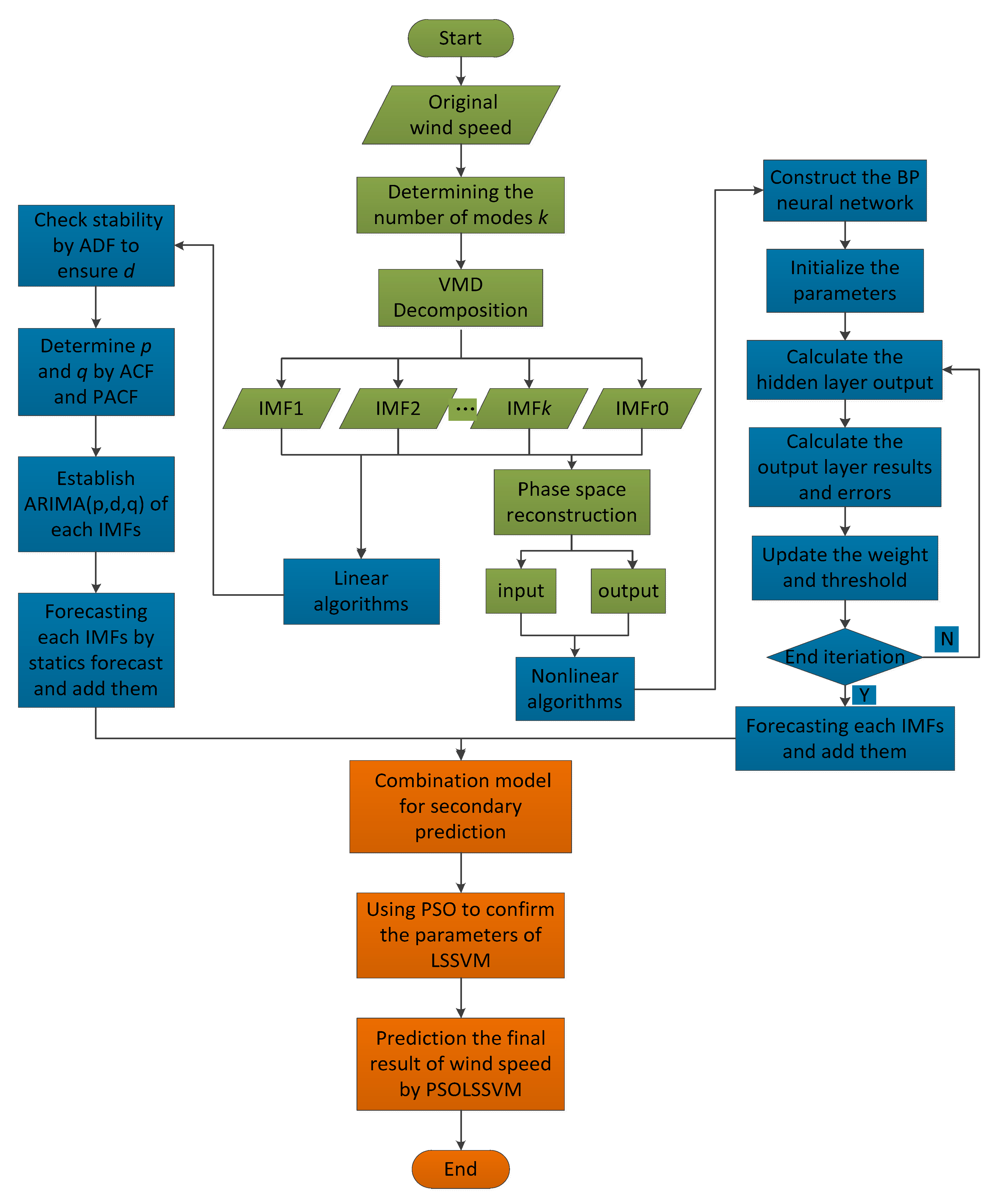
VMD is capable of defining the relevant bands adaptively and balancing the errors between the modes. The solid mathematical foundation that this non-recursive decomposition owns means it could display the local features of the signal effectively. Phase space reconstruction uses delay time to reconstruct the raw time series for maintaining the geometry and dynamic characteristics like the original system. ARIMA is a simple and convenient model that only requires endogenous variables could predict wind speed, but it could not capture nonlinear relationships very well. BP has strong distribution and storage ability to approximate complex nonlinear relationship substantially. However, plenty of parameters need to be fixed to ensure the accuracy of BP, so that the initial values will affect the credibility and acceptability of the results greatly. SVM could avoid the local minimum point and the structure selection of neural network; besides, two vital parameters can be optimized by PSO. Nonetheless, PSOLSSVM also has problems such as unclear directionality and low target during particle searching. According to the merits and demerits summed above, combining all models can give full play to the advantages of each model, and the place where a single model is defective will be compensated by other models. The main steps of the proposed combination model are listed below, and the flowchart is shown in Figure 2. The green part indicates the data processing process, blue indicates linear–nonlinear single prediction models, and orange represents the combination prediction model of PSOLSSVM.

According to all the analysis above, the combination model VMD-P-(ARIMA, BP)-PSOLSSVM is proposed. Research in this paper is based on three hypotheses: (a) Hypothesis 1—VMD and phase space reconstruction can achieve excellent effects, more so than any other data processing methods. (b) Hypothesis 2—regarding the prediction results of the linear–nonlinear single models as the input of the nonlinear combination prediction can effectively improve the accuracy and reliability of the prediction. (c) Hypothesis 3—the PSOLSSVM method for secondary prediction can make up for the shortcomings of the individual prediction models, and this nonlinear prediction is much more accurate than the linear weighted combination.

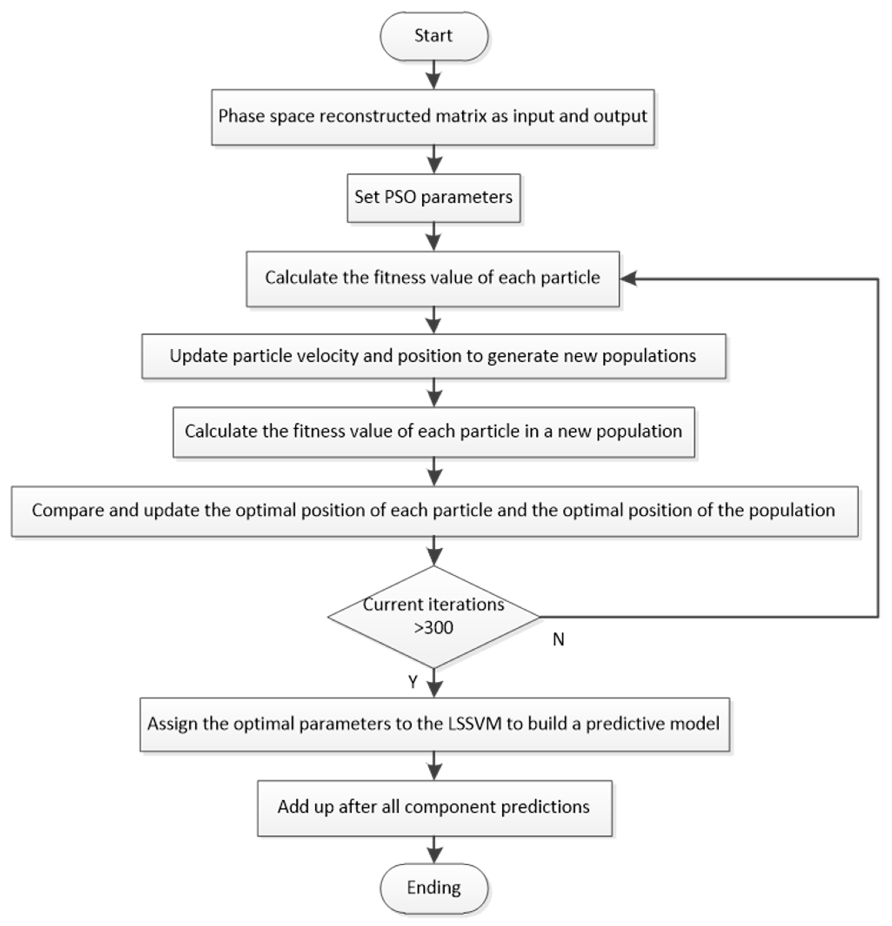
Firstly, VMD is applied to decompose the original wind speed and obtain more stable components. The number of modes k is mainly determined by the difference between the center frequencies of IMF (k) and IMF (k − 1). When the difference tends to stabilize, the value of k can be determined to obtain k patterns and a residual term, and the next step is to reconstruct the phase space for each IMF. The application of C-C method could arrange delay time $\tau$ and embedding dimension $m$ simultaneously and thereby define the input–output matrices of the prediction models. Thirdly, predict the k + 1 IMFs separately by paralleling ARIMA and BP methods. The prediction of ARIMA only needs original IMFs so reconstruction is optional. The detailed ARIMA construction is utilizing unit root test to define d, exploiting ACF and PACF to determine q and p partly, and then finishing the model construction and making a static prediction. The most significant parameter of BP neural network is the number of hidden layers. In order to ensure the accuracy of a single model, we conducted multiple BP network training and determined the best quantity according to accuracy of the test set. Adding up the prediction results of every IMF can obtain the prediction results of the individual models. The fourth step is to perform combined prediction with PSOLSSVM, which optimizes the parameters through the PSO and then uses the trained network for data prediction. Different with separate models, the input values of combined prediction are the prediction results of ARIMA and BP.

4. Short-Term Wind Speed Forecast

4.1. Data Collection

The applicability of the model presented in this paper should be confirmed by processing the actual data. To achieve the goal, the wind speed data are collected from the wind farm of Cheng De, of which the measured height is 70 m and the time interval is 5 min. Because the most representative windy season of Cheng De is winter, the article selects 1000 data from 1 January 2017 as samples; among which, the first 800 data are training sets, and the remaining 200 are used as prediction values. The error analyses of last 100 data are treated to prove the superiority of the combined model. Relevant statistics of 1000 data are described in

Table 1. Statistics information of data.

Mean (m/s)	Max. (m/s)	Min (m/s)	Var.	Skew.	Kurt.
6.4097	12.09	0.87	5.328	0.1027	−0.8186

and Figure 3. The decomposition program and most of the prediction models in the study are implemented in MATLAB 2018a. However, the ARIMA model uses EVIEWS 7 software, and the operating environment is Windows10 Professional.

4.2. Data Processing

It is crucial to set the number of modal components k and the penalty factor $\alpha$, where k directly determines whether the decomposition is correct [54]. According to the study of [55], the conclusion could be made that it is an effective method to select the optimal mode number by using the difference $\Delta f$ between the center frequencies of the components. The criterion for stopping decomposes is when the $\Delta f$ between IMF (k) and IMF (k − 1) decreases gradually and tends to be stable.

Table 2. Center frequency corresponding to different mode number, k.

K	IMF1	IMF2	IMF3	IMF4	IMF5	IMF6	IMF7	$\Delta \mathit{f}$
1	0.0002	-	-	-	-	-	-	-
2	0.0001	0.2597	-	-	-	-	-	0.2596
3	0.0001	0.0197	0.2759	-	-	-	-	0.2562
4	0.0001	0.0125	0.0357	0.2769	-	-	-	0.2412
5	0.0001	0.0125	0.0357	0.2744	0.3860	-	-	0.1116
6	0.0001	0.0100	0.0247	0.0622	0.2756	0.3870	-	0.1115
7	0.0001	0.0100	0.0244	0.0591	0.1383	0.2790	0.4080	0.1290

shows the process of determining k in this case.

It can be seen from Table 2 that this case should be decomposed into five modes on account of the $\Delta f$ between $k=4$ and $k=5$ becoming smaller suddenly. If they continue to decompose, the value of $\Delta f$ may go up instead of down, meaning the center frequency of the adjacent modes is too close and the decomposition will begin aliasing. Based on the above analysis, the optimal number of decompositions is 5, with an additional error term, so the study of this data is based on these six IMFs. The waveform of the obtained six IMFs is shown in Figure 4.

The study also uses the most popular decomposition method, EMD, to process this case for comparing with VMD. EMD can decompose the appropriate mode adaptively, and because of its completeness, the sum of the components is always the same as the source data without residual term. Eight components are obtained by EMD and the specific results are shown in Figure 5.

The IMFs obtained by VMD should be reconstructed in the phase space to receive the input–output matrix of each component. The first thing is calculating the reconstruction parameters one by one. With the help of C-C, the delay time $\tau$ and embedding dimension $m$ of per IMF decomposed by VMD is shown in

Table 3. Phase space reconstruction parameters for each component.

	IMF1	IMF2	IMF3	IMF4	IMF5	IMFR0
m	3	3	5	3	4	5
$\tau$	6	5	3	6	5	2
${\tau }_w$	12	9	12	12	15	7

.

Taking the IMF1 as an example, input–output matrix of the prediction models are Equations (18) and (19). The rest of the IMFs are similar to IMF1.

$$\left[\begin{array}{c}{X}_1\\ X_2\\ ⋮\\ X_{987}\end{array}\right]=\left[\begin{array}{ccc}{x}_1& x_7& x_{13}\\ x_2& x_8& x_{14}\\ ⋮& ⋮& ⋮\\ x_{987}& x_{993}& x_{999}\end{array}\right]$$

(18)

$$\left[\begin{array}{c}{x}_{14}\\ x_{15}\\ ⋮\\ x_{1000}\end{array}\right]$$

(19)

The matrix needs to be divided into a training set and prediction set for data simulation. Specific settings of each IMF are shown in

Table 4. Training set and prediction set settings for each intrinsic mode function (IMF).

Datasets	IMF1	IMF2	IMF3	IMF4	IMF5	IMFR0
Training set	$X_1~X_{787}$	$X_1~X_{789}$	$X_1~X_{787}$	$X_1~X_{787}$	$X_1~X_{784}$	$X_1~X_{791}$
Prediction set	$X_{788}~X_{987}$	$X_{790}~X_{989}$	$X_{788}~X_{987}$	$X_{788}~X_{987}$	$X_{785}~X_{984}$	$X_{792}~X_{991}$

.

Reconstruct the components acquired by EMD according to the same step could get the parameters and data settings as shown in

Table 5. Reconstruction parameters and datasets of raw data and IMFs decomposed by EMD.

IMFs	m	$\mathit{\tau }$	${\mathit{\tau }}_{\mathit{w}}$	Training Set	Prediction Set
O	3	6	7	$X_1~X_{787}$	$X_{788}~X_{987}$
IMF1	2	3	5	$X_1~X_{796}$	$X_{797}~X_{996}$
IMF2	4	6	20	$X_1~X_{781}$	$X_{782}~X_{981}$
IMF3	2	7	9	$X_1~X_{792}$	$X_{793}~X_{992}$
IMF4	5	4	18	$X_1~X_{783}$	$X_{784}~X_{983}$
IMF5	4	5	17	$X_1~X_{784}$	$X_{785}~X_{984}$
IMF6	3	10	22	$X_1~X_{779}$	$X_{780}~X_{979}$
IMF7	2	9	11	$X_1~X_{790}$	$X_{791}~X_{990}$
IMF8	3	10	22	$X_1~X_{779}$	$X_{780}~X_{979}$

.

4.3. Wind Speed Forecast by Separate Models

4.3.1. ARIMA Forecast

ARIMA is a statistics model for linear analysis and prediction; it analyzes the IMFs directly rather than the reconstructed sequences, but this model requires a certain stability of the data to ensure its prediction accuracy. In this paper, ADF (augmented Dickey–Fuller) is employed to test the stability of components so as to decide the difference number d. Supposing the significance level is 1%, this means that if the absolute value of t is greater than that of the critical value, it could estimate that data are stationary. If the absolute value of t is smaller, this indicates that the component is unstable, so it needs to perform the first-order difference and repeat the above steps until the requirement of rejecting the null hypothesis is satisfied. Because the components decomposed by VMD and EMD are more stable and have different frequencies and different periods, some of them can pass the stability test without differential processing, which denotes d = 0. For smooth data or differential data, q and p are determined according to the tailing or truncation of the ACF and PACF. The specific identification method is shown in

Table 6. The identification of autoregressive moving average (ARMA) method.

ACF	PACF	Model Identification
Trailing	p-order truncation	AR(p) model
q-order truncation	Trailing	MA(q) model
Trailing	Trailing	ARMA(p,q) model

.

The ARIMA model structure of each component should be defined before forecasting, therefore, the ADF verification and parameter analysis of each component has been processed in EVIEWS7. Final structures are shown in

Table 7. Autoregressive integrated moving average model (ARIMA) model structures of VMD components.

	IMF1	IMF2	IMF3	IMF4	IMF5	IMFR0
(p, d, q)	(2,2,1)	(4,0,2)	(4,0,2)	(6,0,2)	(2,0,4)	(3,0,5)

.

For comparison, the study also establishes the ARIMA model of original data and EMD components, and the results are expressed in

Table 8. ARIMA model structures of original data and EMD components.

	O	IMF1	IMF2	IMF3	IMF4	IMF5	IMF6	IMF7	IMF8
(p, d, q)	(6,2,1)	(5,0,3)	(5,0,2)	(2,0,4)	(6,2,1)	(2,0,0)	(1,2,0)	(3,4,2)	(6,3,2)

.

The paper utilizes the ARIMA model of every IMF to predict the last 200 data separately. There are two prediction methods when using EVIEWS to establish ARIMA, namely static prediction and dynamic prediction. According to [56], it can be concluded that the effect of dynamic prediction is not as good as static prediction, so this paper chooses static to predict these components. Adding the predicted values of all the IMFs could reconstruct the predicted results of short-term wind speed.

4.3.2. BP Forecast

BP is used to establish nonlinear prediction models for the phase space reconstructed IMFs. Before sending the matrices into the models, the numbers of nodes of three layers need to be confirmed. The numbers of nodes in the input layer should be determined according to the dimension of phase space reconstruction and the output layer with one node. As for the hidden layer, the numbers of nodes are determined due to the input layer separately. The cut-and-try method is mainly used. The reference equation is Equation (20).

$$m=\sqrt{n+1}+a$$

(20)

where $n$ denotes the number of input layer nodes, $m$ represents the number of hidden layer nodes, 1 is the number of output layer node, and $a$ is a constant of 0–10. After several processing, the paper chose six as the number of hidden layer nodes, because the output of the six hidden layers has the smallest error and the highest precision. The other parameters are set as follows: The number of iterations is 100, the learning rate is 0.01, and the error target is 0.00004. After determining model structure and parameters, BP training is carried out for each IMF. The trained model can be used to predict the last 200 data by function sim in order to obtain the short-term prediction results.

4.4. Combined Forecast

A total of 200 data predicted by the two methods served as input of the combined prediction, and the output is still the actual wind speed. In the secondary prediction, the training set is the first 100 data, and the other 100 are the final prediction set. The final prediction of this study is based on the PSOLSSVM, which exploits PSO to optimize the combination of $\sigma$ and $\gamma$. In the case of the parameters of PSO, the optimization interval of $\mathsf{\gamma }$ is set to [0.1, 300], and the optimization interval of $\mathsf{\sigma }$ is [0.1, 100], the number of iterations is adopted as 300, speed of particle optimization is 25, population is 20, initial weight is 0.9, and the final weight is set as 0.4. In addition, in order to evaluate the performance of the proposed model proposed in this paper, two linear weighted combinations including AW (average weighted) and EW (error weighted) are used as the comparisons. Using three preprocessing methods of the original data into the same prediction model could obtain the optimal processing method. The PSOLSSVM optimal parameters are listed in

Table 9. Optimal parameters obtained by particle swarm optimization.

	VMD-P-(ARIMA, BP)-PSOLSSVM	EMD-P-(ARIMA, BP)-PSOLSSVM	O-P-(ARIMA, BP)-PSOLSSVM
$\gamma$	239.25	207.40	248.40
σ	26.27	67.89	57.60

.

5. Results and Discussions

5.1. Model Performance Evaluation

It is valuable to employ a few error indicators when judging the prediction ability of the proposed model. Six indicators have been selected to evaluate the prediction results of the last 100 data. Statistical error measures such as MAE (mean absolute error), MAPE (mean absolute percent error), and RMSE (root mean squared error) are applied to assess the model according to the error between the predicted and actual values. Calculation equation is shown in (21)–(23).

$$MAE=\frac{1}{N}{\displaystyle \sum }_{i=1}^N\left|y_i-{\widehat{y}}_i\right|$$

(21)

$$MAPE=\frac{1}{N}{\displaystyle \sum }_{i=1}^N\left|\frac{y_i-{\widehat{y}}_i}{y_i}\right|\ast 100\%$$

(22)

$$RMSE=\sqrt{\frac{1}{N}{\displaystyle \sum }_{i=1}^N{\left(y_i-{\widehat{y}}_i\right)}^2}$$

(23)

where ${\widehat{y}}_i$ denotes the predicted value of the wind speed, $y_i$ represents the actual wind speed, and the value of N is 100 in this paper, which denotes the number of the error analysis.

To further describe the meliority of the combination model in this study and the indispensability of each step, improved percentages indicators including $P_{MAE}$, $P_{MAPE}$, and $P_{RMSE}$ are introduced to measure the amendment degree. The improvement indicators are designed as below:

$$P_{MAE}=\frac{MA{E}_1-MA{E}_2}{MA{E}_1}\ast 100\%$$

(24)

$$P_{MAPE}=\frac{MAP{E}_1-MAP{E}_2}{MAP{E}_1}\ast 100\%$$

(25)

$$P_{RMSE}=\frac{RMS{E}_1-RMS{E}_2}{RMS{E}_1}\ast 100\%$$

(26)

5.2. Error Comparison Analysis

Intending to test the excellence of the proposed model named VMD-P-(ARIMA, BP)-PSOLSSVM, multiple models are opted for error comparison analysis, including two separate models called VMD-ARIMA, VMD-P-BP, two combined model using different combination methods like VMD-P-(ARIMA, BP)-AW, VMD-P-(ARIMA, BP)-EW, and two different preprocessing methods named EMD-P-(ARIMA, BP)-PSOLSSVM and O-P-(ARIMA, BP)-PSOLSSVM. Statistical indicators of all seven methods are listed in

Table 10. Error indicators of all models.

NO.	Model	MAE (m/s)	MAPE (%)	RMSE (m/s)
M1	VMD-ARIMA	0.1134	3.5035	0.14955
M2	VMD-P-BP	0.2039	6.7225	0.25828
M3	VMD-P-(ARIMA,BP)-AW	0.1466	4.7203	0.1921
M4	VMD-P-(ARIMA,BP)-EW	0.1336	4.2618	0.1767
M5	VMD-P-(ARIMA,BP)-PSOLSSVM	0.0524	2.0055	0.0715
M6	EMD-P-(ARIMA,BP)-PSOLSSVM	0.0605	2.3106	0.0812
M7	O-P-(ARIMA,BP)-PSOLSSVM	0.0707	3.1773	0.1175

and the best prediction results are marked in bold.

For observing the prediction accuracy intuitively, the study turns the content in

Table 11. The statistics information of supplementary case.

Mean (m/s)	Max. (m/s)	Min (m/s)	Var.	Skew.	Kurt.
5.3123	16.63	0.37	11.417	0.9119	−0.0162

into three bar charts. In Figure 6, Figure 7 and Figure 8, the green bars represent separate prediction models, blue represents other combined models, and red denotes the proposed combined model with different preprocessing. It can be found that three indicators of M5 is the minimum among all methods, which means the proposed model is the best in terms of precision and stability. In the next analysis, the prediction results of all methods are grouped and evaluated to prove that each part of the proposed model is reasonable.

From observing Figure 9 and the comparison of the proposed and the separate models including M1 and M2, it can be detected that the MAE, MAPE, and RMSE of the M5 are virtually all less than those of the relevant separate models for the three horizons. As for the separate models, the performance of ARIMA is more accurate and stable than the BP. Compared with the ARIMA, $P_{MAE}$ of the proposed model is 53.8% while $P_{MAPE}$ and $P_{RMSE}$ is 42.8% and 52.2%, respectively. Simultaneously, matched with the result of BP, the value of $P_{MAE}$, $P_{MAPE}$, and $P_{RMSE}$ of the M5 is 74.3%, 70.2%, and 72.3% separately. Among this analysis, $P_{MAE}$ of three improved indicators is the maximum indicator that the proposed has a prominent contribution to increase the prediction accuracy. In the way of improving stableness, the proposed also has outstanding behavior, which may make some efforts to decrease the effect of wind power when entering the grid. Comparing the M1 with M2, 44.4%, 47.9%, and 42.1% correspond to $P_{MAE}$, $P_{MAPE}$, and $P_{RMSE}$ of the M1. The reason of this situation is because the signal decomposition technique treats the previously volatile wind speed into more stable series, so the linear model ARIMA could extract the signal preferably. Thereby, decomposition improves the accuracy and stability of the model to some extent. The analysis in this paragraph mainly expresses that the combined model in this paper is much better than the separate models from the accuracy and stability. In particular, the comparison not only shows that the outstanding contribution of PSOLSSVM during the secondary prediction, but also indicates the high volatility of wind speed after VMD processed can be dismissed partly. Individual prediction models have their own inherent characteristics, which causes them to have different merits and demerits in prediction. Different methods will collect different information from the data, so the separate models may ignore some information and only extract what it considers important. Thereby, using ARIMA and BP results as the input of the secondary prediction can optimize the individual models, while some defects and the inaccuracies of them can be complemented by the combination model; thus, the accuracy and stability of the prediction will be improved.

Figure 10 plots the predictions and the errors of the M3, M4, and M5 with the corresponding improvement indicators of them. The contrast of three combination models emphasizes the supremacy of the PSOLSSVM as the secondary prediction method. Linear weighting just averaged the results of two separate models to some extent, and the same for the errors, so it is difficult to play up strengths and avoid weaknesses. Moreover, the results of the individual models still have obvious nonlinear characteristics, thus, the prediction effect of the linear is theoretically inferior to the nonlinear combination. Using PSOLSSVM as the combination method is better than the linear weighted according to the study, which the $P_{MAE}$, $P_{MAPE}$ and $P_{RMSE}$ of the proposed model are all more than 50% compared to the AW and EW. The relevant value of proposed are 64.3%, 57.5%, and 62.8% for AW and 60.8%, 52.9%, and 59.5% for EW. Result of the EW is better than the AW because EW decreases the weight of the method with large error to a certain extent and increases that of the high precision. The $P_{MAE}$, $P_{MAPE}$, and $P_{RMSE}$ of M4 compared with M3 is 8.9%, 9.7%, and 8.1%. From the above analysis, it can be summarized that the secondary prediction method proposed in this paper is much more excellent than the linear weighting of the separate models and the PSOLSSVM improves much in precision and stability based on the $P_{MAE}$, $P_{MAPE}$, and $P_{RMSE}$ analysis.

M5, M6, and M7 have diverse pretreatments with the one prediction procedure M6 is decomposed by EMD and M7 utilizes original data directly, the relevant error comparison and improvement indicators are shown in Figure 11, The key point of the proposed model is the secondary prediction using the first results of the separate models, so comparing the different inputs of the first prediction will find the best decomposition method to upgrade the accuracy of the whole model. Sort results can be achieved by comparing the worst effect of the combination prediction using the original data, followed by the EMD, and the best is the proposed model in this study. The $P_{MAE}$ of the proposed compared with M7 is 25.9%, $P_{MAPE}$ is 36.9%, and $P_{RMSE}$ is 39.1%, and the same analysis with M6 has the relevant value of, respectively, 13.3%, 13.2%, and 11.9%. Furthermore, EMD battles with the original data to get the $P_{MAE}$, $P_{MAPE}$, and $P_{RMSE}$ at 14.5%, 27.2%, and 30.9%. Improvement degree in this group is smaller than the last comparison group, which represents that the preprocessing have weaker improvement ability than the secondary prediction. This diagnosis proved the validity and necessity of data processing for VMD and phase space reconstruction. For a wind speed sequence with large fluctuations, it is effective to decompose original data into stable components by some methods, and then prediction. On account of the excellent impact and strong mathematical principle of VMD, this paper combines it with phase space reconstruction to process wind speed data.

In summary, VMD-ARIMA is the better model in separate predictions because of the available decomposition and the useful linear prediction; secondary prediction of the proposed model can greatly optimize the combination of the separate models, while the optimized degree is superior to the linear weighting; PSOLSSVM suffices to compensate the shortcomings of individuals and capture the nonlinear information to enhance the prediction accuracy and stability; VMD is a novel and eligible technology to improve this combination model from the source; the optimization effect of the secondary prediction is higher than the VMD or any other combinations.

6. Additional Forecasting Case

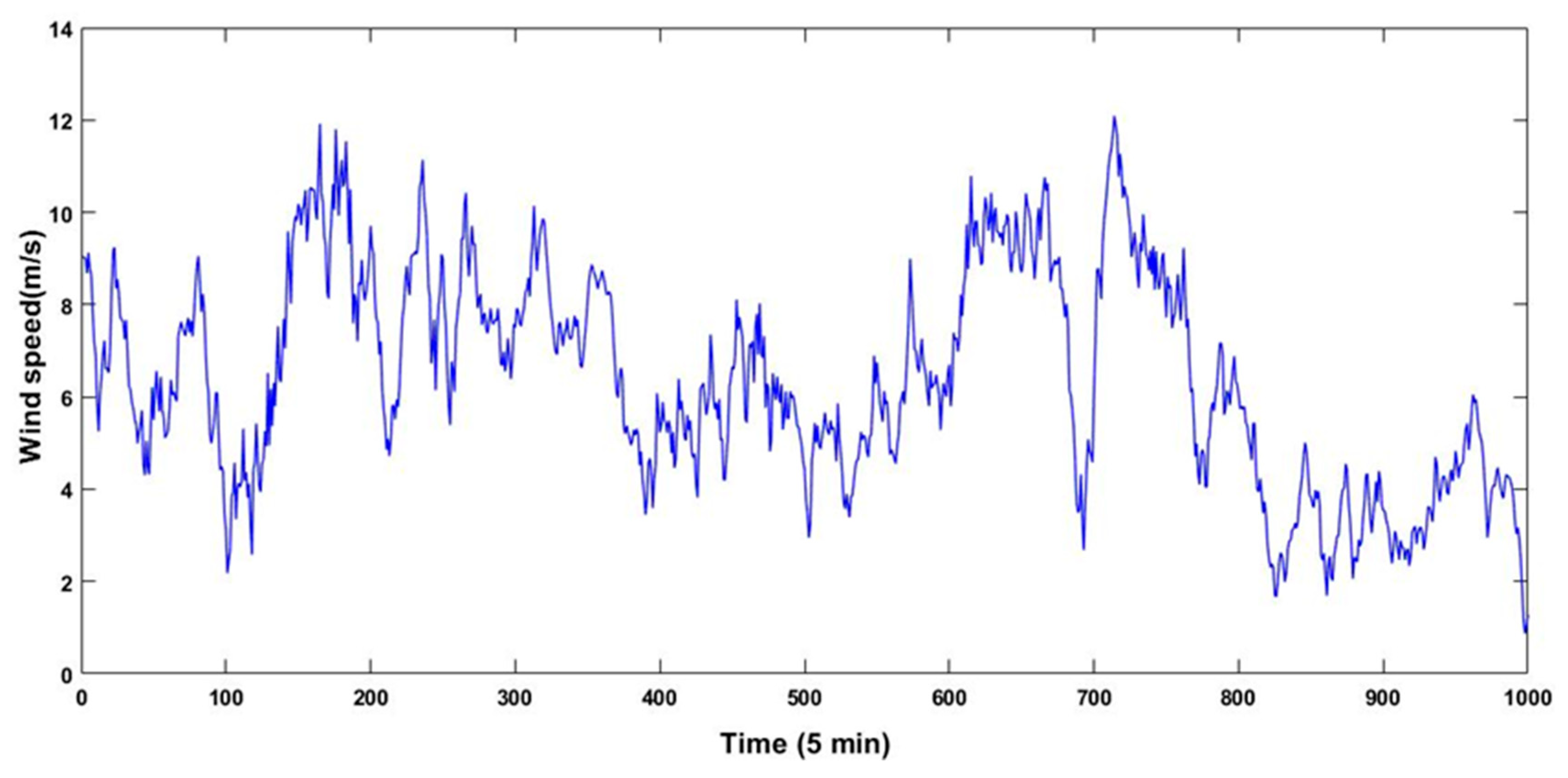
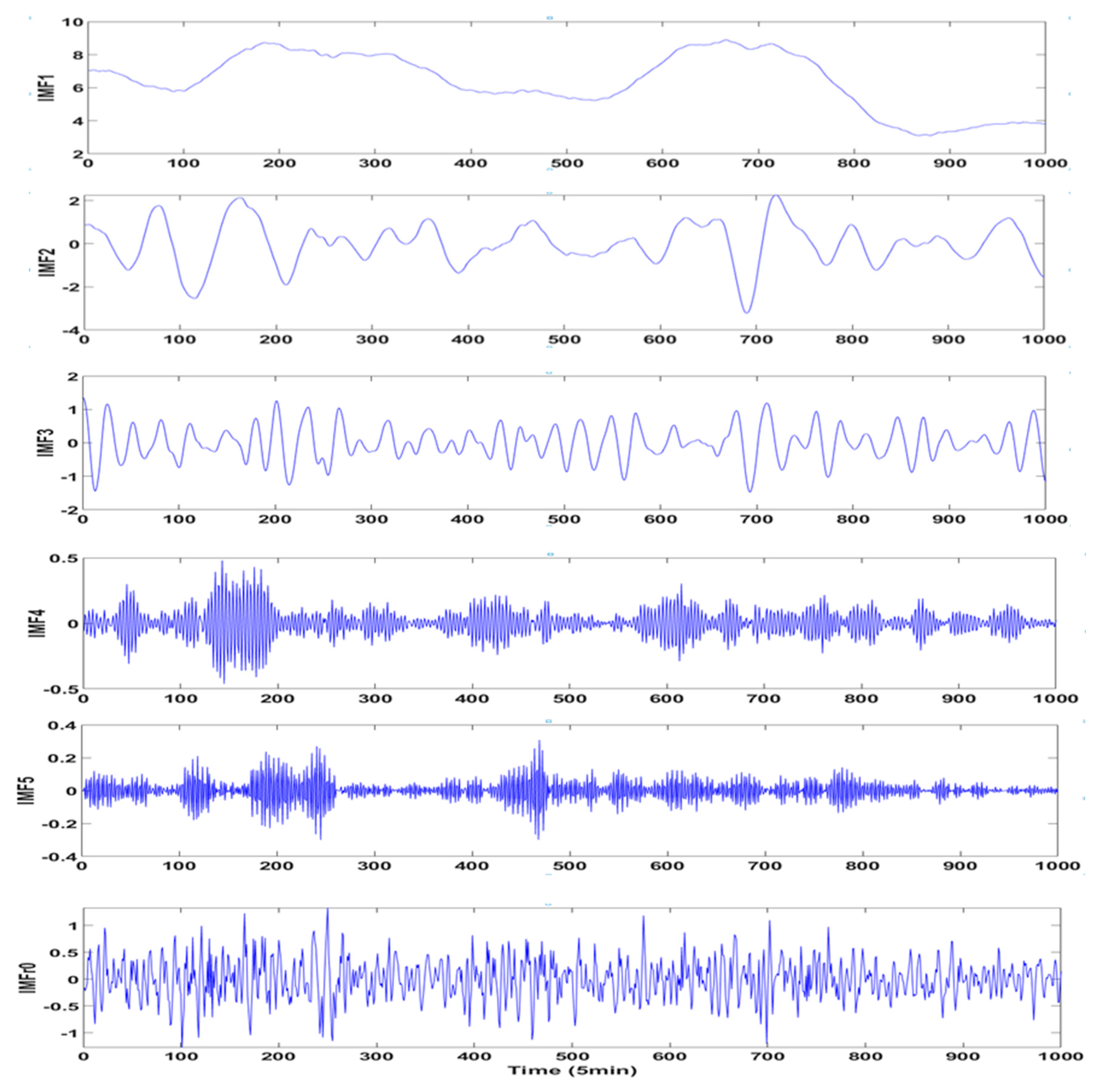
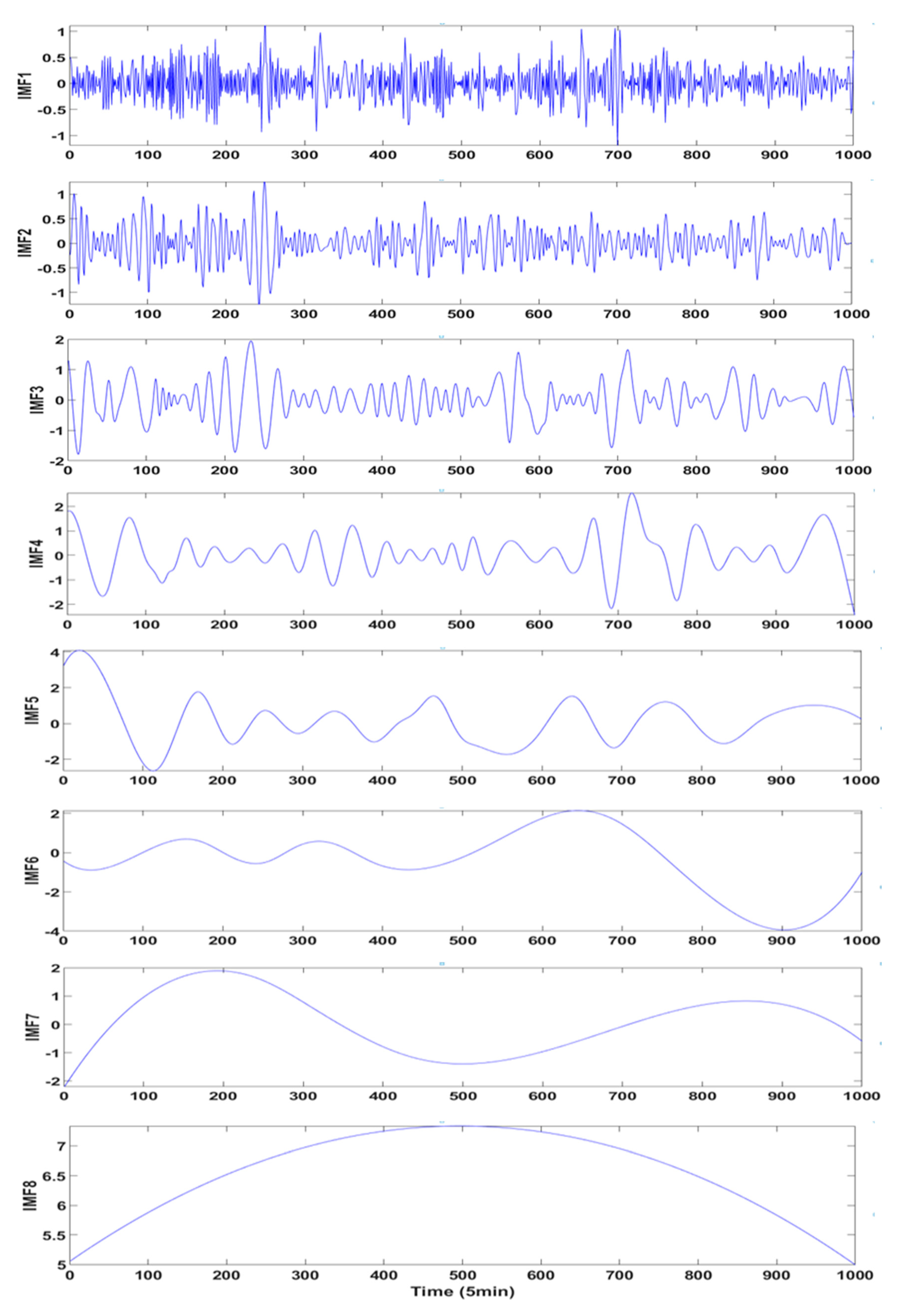
The universality and applicability must be proofed when a novel method proposed, so the spring data from the same district is applied to complete the study. In consideration of the most fluctuating wind speed, 1000 data start from 30 March of 2017 are picked as a supplementary case. After decomposition, six components and one residual term are obtained by VMD and nine components by EMD, and the specific phase space reconstruction and prediction steps are omitted for the sake of avoiding the duplication. The statistical information and the final prediction results are exhibited in Table 11 and

Table 12. Supplementary case prediction results analysis.

NO.	Model	MAE (m/s)	MAPE (%)	RMSE(m/s)
M1	VMD -ARIMA	0.1270	4.0226	0.1571
M2	VMD-P-BP	0.2028	6.4086	0.2487
M3	VMD-P-(ARIMA,BP)-AW	0.1572	4.9628	0.1956
M4	VMD-P-(ARIMA,BP)-EW	0.1483	4.6838	0.1851
M5	VMD-P-(ARIMA,BP)-PSOLSSVM	0.0591	1.8937	0.0729
M6	EMD-P-(ARIMA,BP)-PSOLSSVM	0.0682	2.1712	0.0887
M7	O-P-(ARIMA,BP)-PSOLSSVM	0.1124	3.6340	0.1389

, respectively.

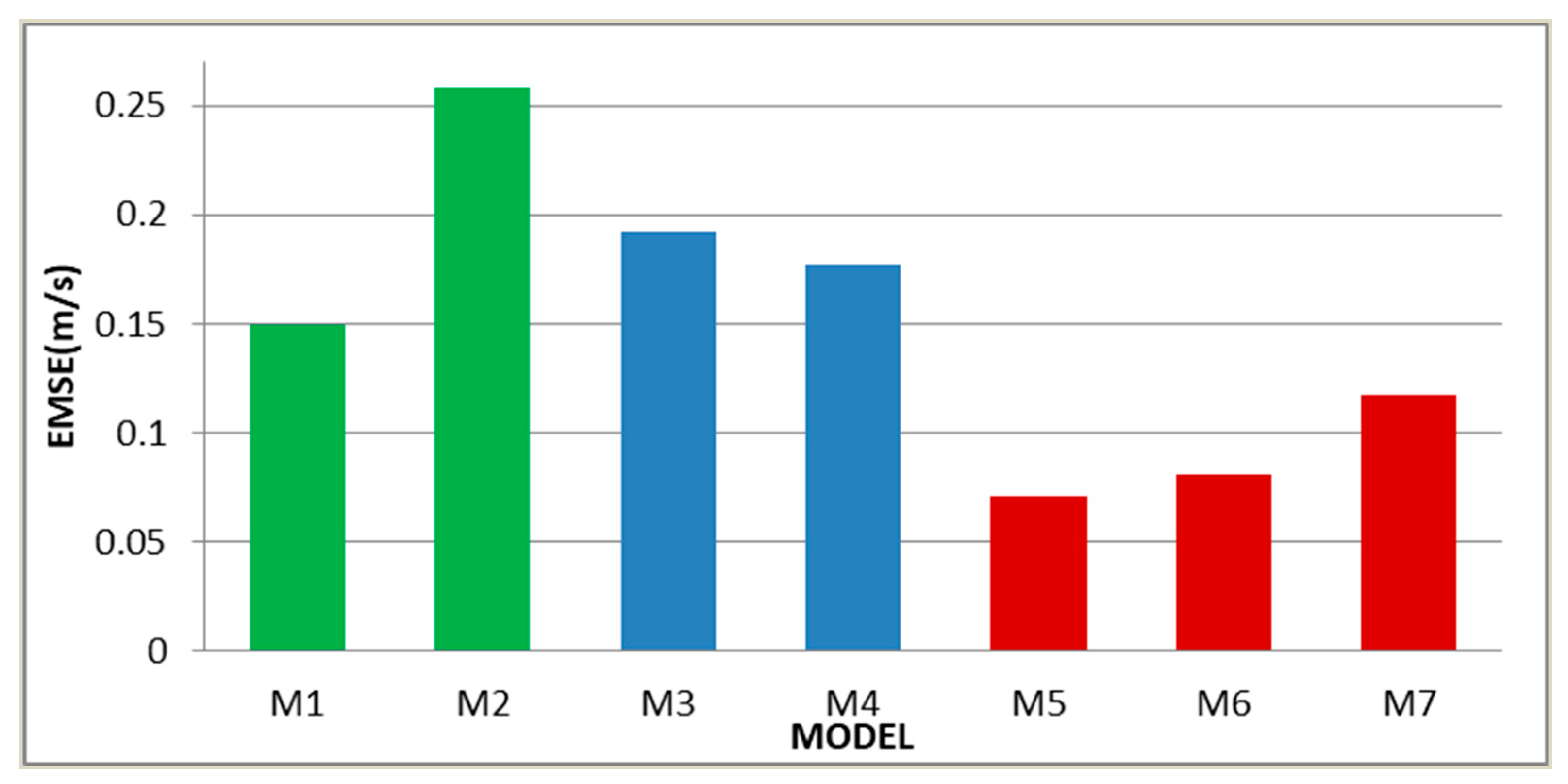
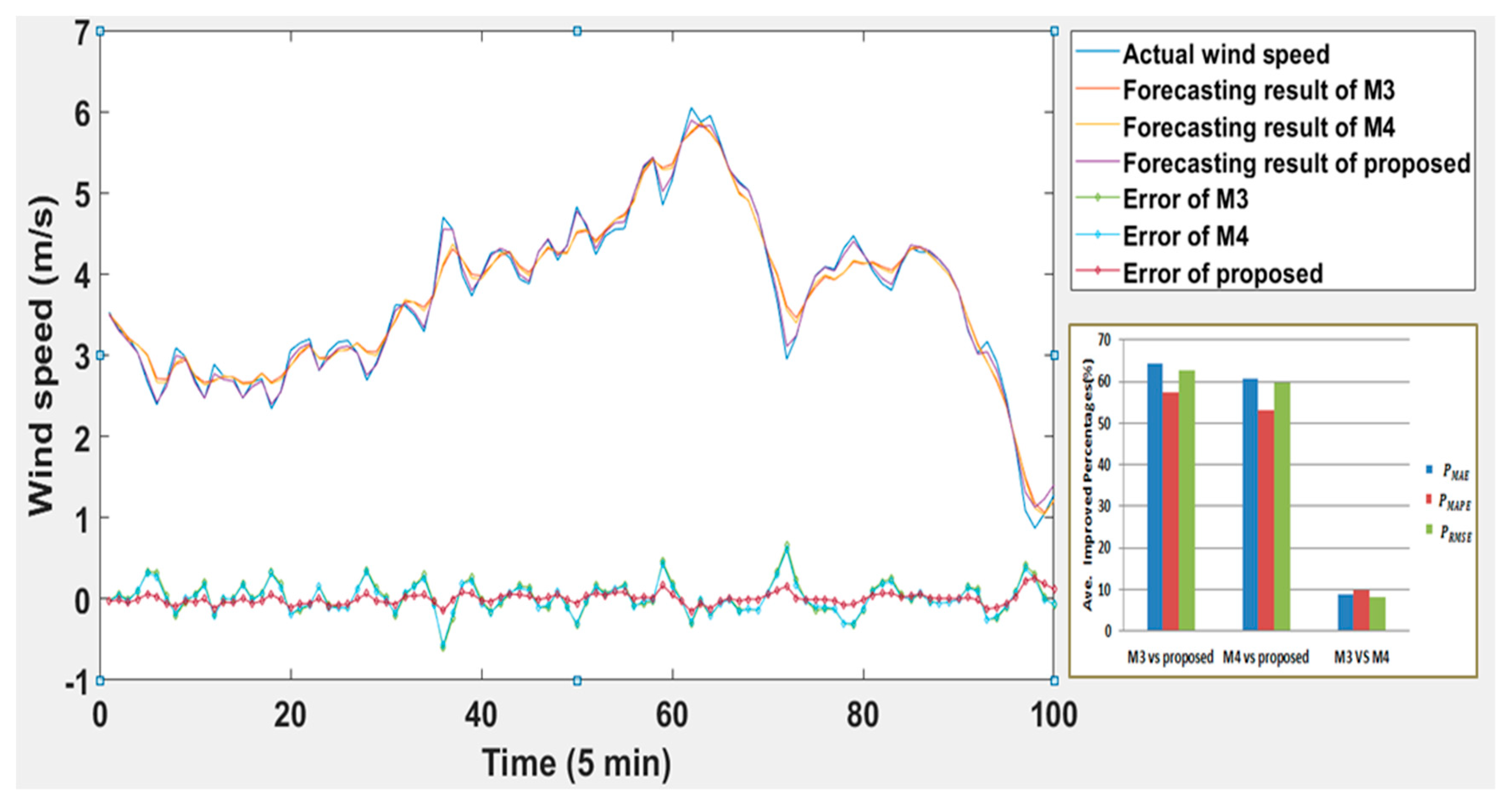
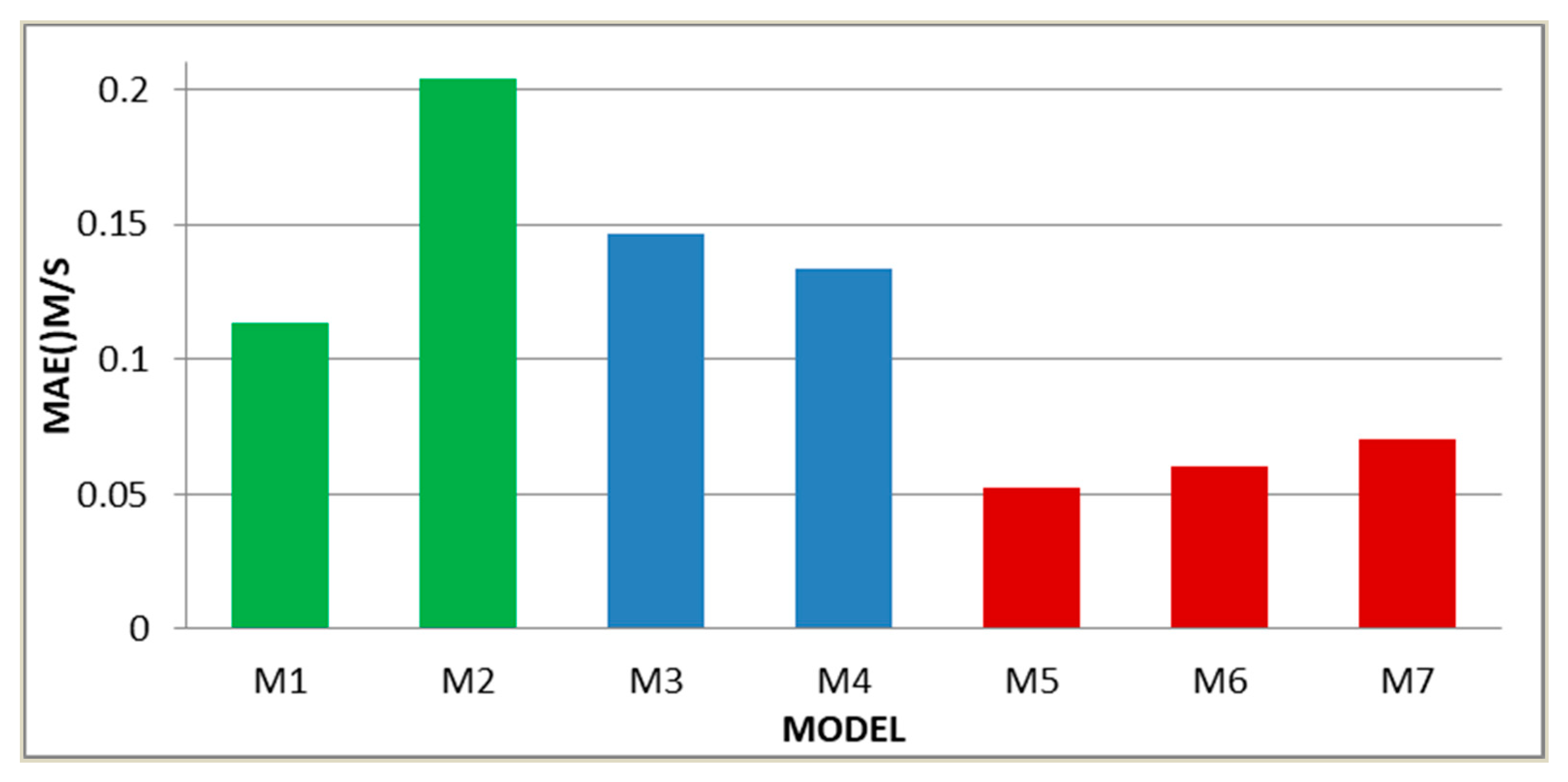
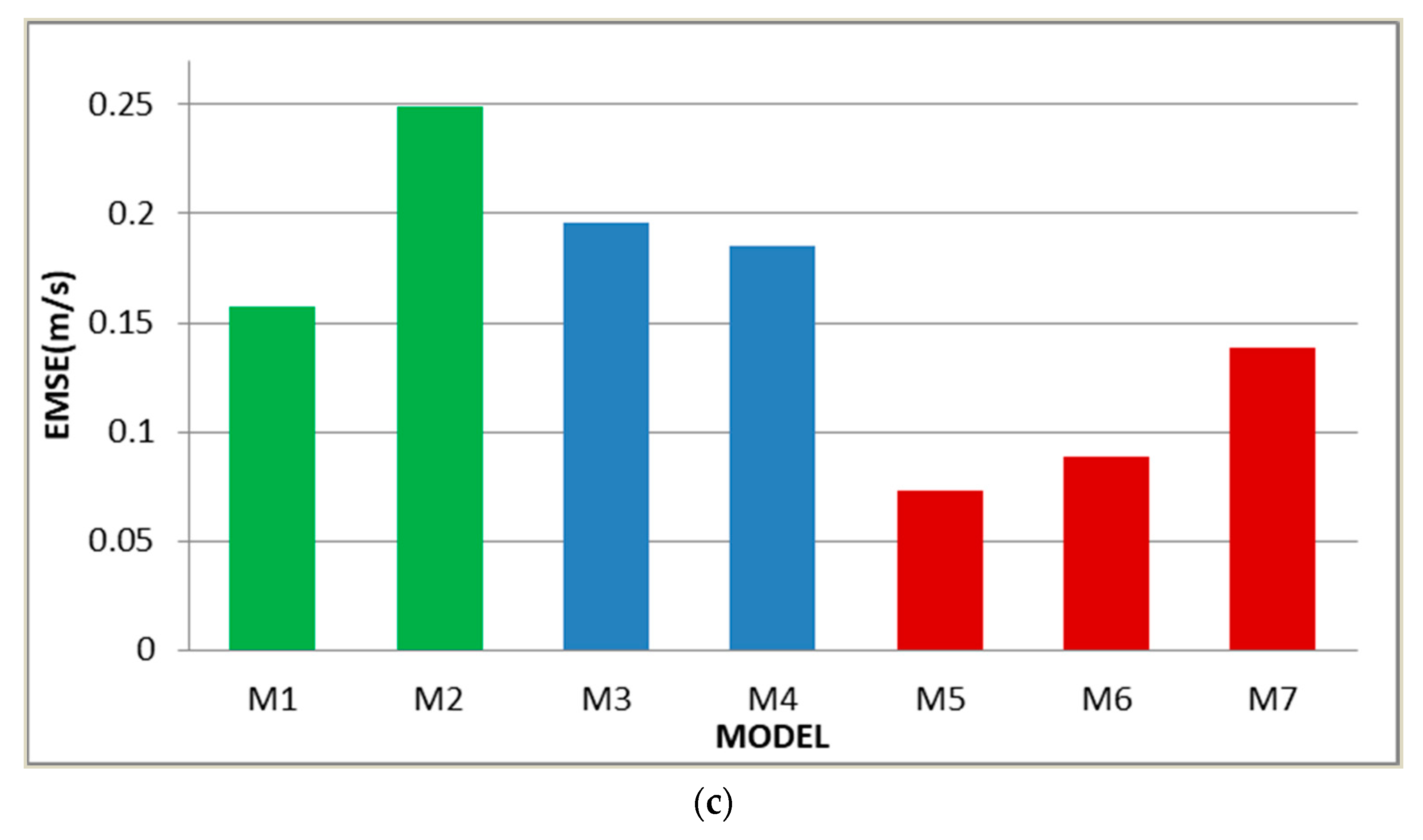
Different resources receive different prediction results is a natural phenomenon, while the error analysis results of the supplementary case are consistent with the main case to some extent. Original data of the supplementary case is more volatile, which makes the prediction precision and reliability of the proposed model lower than the previous case. But the model developed in this paper is still the best in the supplementary case according to the results that the value of MAE, MAPE, and RMSE is 0.0591 m/s, 1.8937%, and 0.0729 m/s, respectively. ARIMA is still the better one in the separate models, and the improved indicators of it compared with BP are 37.4%, 37.2%, and 36.8%. The secondary prediction in this case manifests much better than the linear weighted, which the performance is ranked as M5 > M4 > M3, where > represents better. For instance, the $P_{MAE}$ of the proposed compared with M3 is 62.4%, $P_{MAPE}$ is 61.8%, and $P_{RMSE}$ is 62.7%. When analyzing the M5, M6, and M7, it can be found that the data processed by VMD and phase space reconstruction is more excellent than unprocessed or processed by EMD. Synthetically speaking, the data have more fluctuation when the proposed model has worse results, but is still optimal compared to other methods. Figure 12 and Figure 13 show the specific comparison results and improvement degree of the supplementary case.

On the one hand, the supplementary case proves that the proposed model has universal applicability to short-term wind speed prediction from the aspects of the data processing method, secondary predictive idea, and the final prediction method. By comparing it with other methods, the best results of the proposed method confirm that the requirement of high prediction accuracy and stability has been satisfied. On the other hand, for different data, the performance of the proposed model is different, as well as the degree of improvement. However, though the data with sharp waves will predict poorly, it demonstrates the proposed method is not a completely theoretical application but a practicality one.

7. Conclusions

Precise and credible short-term wind speed prediction is conducive to ensure the stability of the power grid. It is convenient for wind farms to arrange the unit maintenance and maintenance reasonably. Moreover, it will help to promote the development of wind power and improve its competitiveness. This paper developed a novel combination optimization model for short-term wind speed prediction, which the main idea is using the processed data and separate models to predict the wind speed first, and then regarding the results of the separate models as the input of the other method to make a second forecast. VMD and phase space reconstruction were applied as the preprocessing method, of which the former decomposes the wind speed data and the latter determines the input–output matrix of the prediction model. Separate models contain ARIMA and BP, meanwhile the PSOLSSVM with diverse principle is employed to do the secondary prediction. After simulation of two sets of data, this study verifies that the secondary prediction could compensate the shortcomings of the separate models, and the proposed model VMD-P-(ARIMA, BP)-PSOLSSVM is more effective than any other methods in prediction field of short-term wind speed.

Several conclusions can be drawn from this paper: (a) Decomposing the original wind speed by VMD can reduce the instability effectively, and the connection to phase space reconstruction enhances the mathematical basis of the whole model. Chaos method applied with VMD makes the matrix of components decidedly more scientific. The applicability of the process is the confirmation of Hypothesis 1. (b) The biggest innovation of this paper is using the PSOLSSVM and the results of the separate models for secondary prediction, of which the accuracy and reliability surpasses any other models. It also proves that combining linear with nonlinear methods, whose principles are different, can avoid the defects of the individual model and improve the prediction preformance, which prove the correctness of Hypothesis 2. (c) Case studies from two seasons with high fluctuations indicate that the novel model developed in the study has scalable application prospects and can meet the requirements of wind farms. This is the relevant content of Hypothesis 3 in the modeling process, and the error analysis results confirm the correctness of Hypothesis 3. (d) The error results of the two empirical cases in this paper prove that it is a very practical method to predict the short-term wind speed according to the proposed research process and modeling steps. It also demonstrates that the model has universal applicability and wide applicability.