Energy Consumption Analysis and Optimization of the Deep-Sea Self-Sustaining Profile Buoy


1
State Key Laboratory of Precision Measuring Technology and Instruments, Tianjin University, Tianjin 300072, China
2
Shandong University of Science and Technology, Qingdao 266590, China
*
Author to whom correspondence should be addressed.
Energies 2019, 12(12), 2316; https://doi.org/10.3390/en12122316
Submission received: 5 April 2019
/
Revised: 11 June 2019
/
Accepted: 12 June 2019
/
Published: 17 June 2019
Abstract
:In order to reduce the energy consumption of deep-sea self-sustaining profile buoy (DSPB) and extend its running time, a stage quantitative oil draining control mode has been proposed in this paper. System parameters have been investigated including oil discharge resolution (ODR), judgment threshold of the floating speed and frequency of oil draining on the energy consumption of the system. The single-objective optimization model with the total energy consumption of DSPB’s ascent stage as the objective function has been established by combining the DSPB’s floating kinematic model. At the same time, as the static working current of the DSPB can be further optimized, a multi-objective energy consumption optimization model with the floating time and the energy consumption of the oil pump motor as objective functions has been established. The non-dominated sorted genetic algorithm-II (NSGA-II) has been employed to optimized the energy consumption model in the ascent stage of the DSPB. The results showed that the NSGA-II method has a good performance in the energy consumption optimization of the DSPB, and can reduce the dynamic energy consumption in the floating process by 28.9% within 2 h considering the increase in static energy consumption.
1. Introduction
In order to accurately measure the profile data of the global ocean such as temperature and salinity, a global ocean observation and experimental project “ARGO plan” [1,2,3] has been carried out in 2000. Self-sustaining profile detection buoys including the deep-sea self-sustaining profile buoy (DSPB) have been used in this project. The DSPB will work in the sea for more than years years until the power is exhausted and the working depth of which is up to 4000 m. The working life and operation are important for the DSPB because they involve the performance of the buoy and the reliability of the data. Effective reducing the energy consumption of DSPB’s working process is an urgent problem as the limited power supply that DSPB can carry.
The number of works on energy consumption for the DSPB is relatively smaller than similar works for autonomous underwater vehicle (AUV). The working mechanism of the AUV is similar to the DSPB, so related researches of the AUV can be referenced in this paper. The energy consumption optimization of AUVs are mainly from optimizing parameters such as dynamic resistance model, gliding pitch angle and speed, the force applied by thrusters and their opening times [4,5,6,7].
As the movement mode of the DSPB only considers a single degree of freedom, the energy consumption optimization can be developed by reducing the static working current, reducing the dynamic resistance and reducing the dynamic energy consumption by optimizing the motion control mode. Koh et al. [8] have proposed an optimized design process for multi-target model of the buoy for the resonant-type wave energy converter. The multi-objective genetic algorithm has been used to get the Pareto-optimal set and the weighted method has been used to make optimal decisions.
The energy consumption optimization model of AUVs and profile buoys are always established to the multi-objective model as optimization parameters of them are complicated [7,8]. The non-dominated sorted genetic algorithm-II (NSGA-II) method has been widely used in multi-objective optimization problems and has been proved to be one of the most effective algorithms at present [9,10]. The NSGA-II method has been applied in different fields such as power management in HEVs [11], embedded real-time system [12], energy system [13,14,15], power system reconstruction [16], generation expansion planning (GEP) problem [17,18,19], thermal generating optimization problem [20,21], land use scenario [22], machine and engine efficiency problem [23,24].
There is much research about parameter optimization of the multi-objective model with NSGA-II. Krzyszt et al. [25] have proposed a multi-objective optimization of the selected design parameters in a single-family building intemperate climate conditions and optimized by NSGA-II method. Panda [26] has investigated the application of NSGA-II technique for the tuning of a proportional integral derivate (PID) controller for a flexible AC transmission system (FACTS) based stabilizer. Zhong et al. [27] have used the NSGA-II to optimize an organic Rankine cycle with evaporation temperature and condensation temperature as the decision variables. Reed et al. [28] have applied the NSGA-II on a multi-objective long term groundwater monitoring and solved multi-objective optimization problems with only a few simple user inputs automatically. Bogdan et al. [29] have proposed an original method to optimize the reconfiguration of distribution systems considered various criteria with NSGA-II. Lakshminarasimman et al. [30] have used NSGA-II and modified NSGA-II (MNSGA-II) to obtain better compromised solutions of various parameters of cellular base station (BS) placement problem such as site coordinates, transmitting power, height and tilt angle.
In other multi-objective optimization problems, the NSGA-II method can show unique advantages. Mariano et al. [31] have introduced a memetic algorithm based on the NSGA-II to solve the flexible job-shop scheduling problem. Agrawal et al. [32] have used the NSGA-II and its jumping gene (JG) adaptations to solve the design stage optimization of an industrial low-density polyethylene (LDPE) tubular reactor. Gopal et al. [33] have attempted to explore the pervaporation process economics by employing artificial intelligent method of NSGA-II. Ye et al. [34] have used NSGA-II to solve the proposed multi-objective optimization problem around the transient stability constrained optimal power flow (OPF). Agarwal et al. [35] have carried out the optimal design of the shell and tube heat exchanger (HX) and used a compact formulation of the Bell–Delaware method, coupled with NSGA-II-sJG. Bekele et al. [36] have developed an automatic calibration routine and the NSGA-II has been applied to the study on multi-objective automatic calibration of a physically based, semi-distributed watershed model. Nemmani et al. [37] have used NSGA–II to solve the two- objective optimization problem of minimization of the treatment cost with simultaneous maximization of percent removal of toluene. Majumdar et al. [38] have used real-coded NSGA-II to guarantee the maximization of concentration of desired species in a semibatch epoxy polymerization process. Li et al. [39] have used the NSGA-II for power-split plug-in hybrid electric vehicle (PHEV) applications. Sharma et al. [40] have proposed the use of NSGA-II for joint allocation of bits and subcarriers in the downlink of MIMO-OFDMA system. Bahram et al. [41] have used two single-objective and a NSGA-II two-objective genetic algorithms to minimize thermodynamic properties and economic values of the integrated structure, simultaneously. Li et al. [42] have used NSGA-II to solve a type of biobjective bilevel programming problem.
Katiani et al. [43] have used NSGA-II to perform an optimized, coordinated, and selective allocation of control and protection devices in distribution networks with distributed generation (DG). Dai et al. [44] have used NSGA-II to solve Gini-coefficient based stochastic optimization (GBSO). Cavalcante et al. [45] have used NSGA-II to determine non-dominated solutions of an evolutionary multi-objective regenerator placement strategy for elastic optical networks (eMORP). Muhuri et al. [46] have used NSGA-II to solve the multi-objective reliability redundancy allocation problem (MORRAP). Cheraghchi et al. [47] have verified that NSGA-II performs better than other multi-objective optimal evolutionary algorithms (MOEAs) in predicting disruptive factors of Liner shipping through experiments. Paul et al. [48] have used NSGA-II to optimize two cluster validity indices named separation and cohesion. Zhu et al. [49] have developed NSGA-II to explore an optimal design space of Hybrid electric propulsive systems (HEPSs). Wang et al. [50] have proved that the novel crash box optimized by NSGA-II can improve the energy absorption characteristics and comprehensive crashworthiness more effectively, and make the collision process controllable and stable. Lotfi et al. [51] have applied NSGA-II to solve both cell planning and joint cell and backhaul planning problem to minimize the cost of planning, while maximizing the coverage simultaneously.
In order to effectively improve the service life of the DSPB, the energy consumption of the DSPB’s whole working process has been analyzed in this paper. The stage quantitative oil draining control mode has been innovatively adopted to replace the traditional one-time oil draining method. The single-objective optimization model has been established based on the DSPB’s floating kinematic model with the total energy consumption of DSPB’s ascent stage as the objective function. In order to enhance the applicability of the energy consumption optimization model, the multi-objective optimization model has been established with the floating time and energy consumption of oil pump motor as objective functions. The multi-objective optimization model can be suitable for different static working current as the static working current of the DSPB can be further optimized. Key parameters contain oil discharge resolution (ODR), judgment threshold of the floating speed and frequency of oil draining have been considered as the decision variables. The NSGA-II method has been employed to optimize the parameters and minimize the energy consumption of the DSPB’s ascent stage. The traversal method has been adopted to verify the accuracy and timeliness of the NSGA-II method.
2. Analysis Methods
The first section of this chapter will analyze the energy consumption of the DSPB, the second section will establish the kinematics model of the DSPB, the third section will combine the kinematics model of the DSPB to establish the energy consumption model, and the fourth section will introduce the workflow of the stage quantitative oil draining control mode, the fifth section will combine the stage quantitative oil draining control mode to establish energy optimization models, and the sixth section will introduce the optimization method of the energy optimization models.
2.1. Energy Consumption Analysis
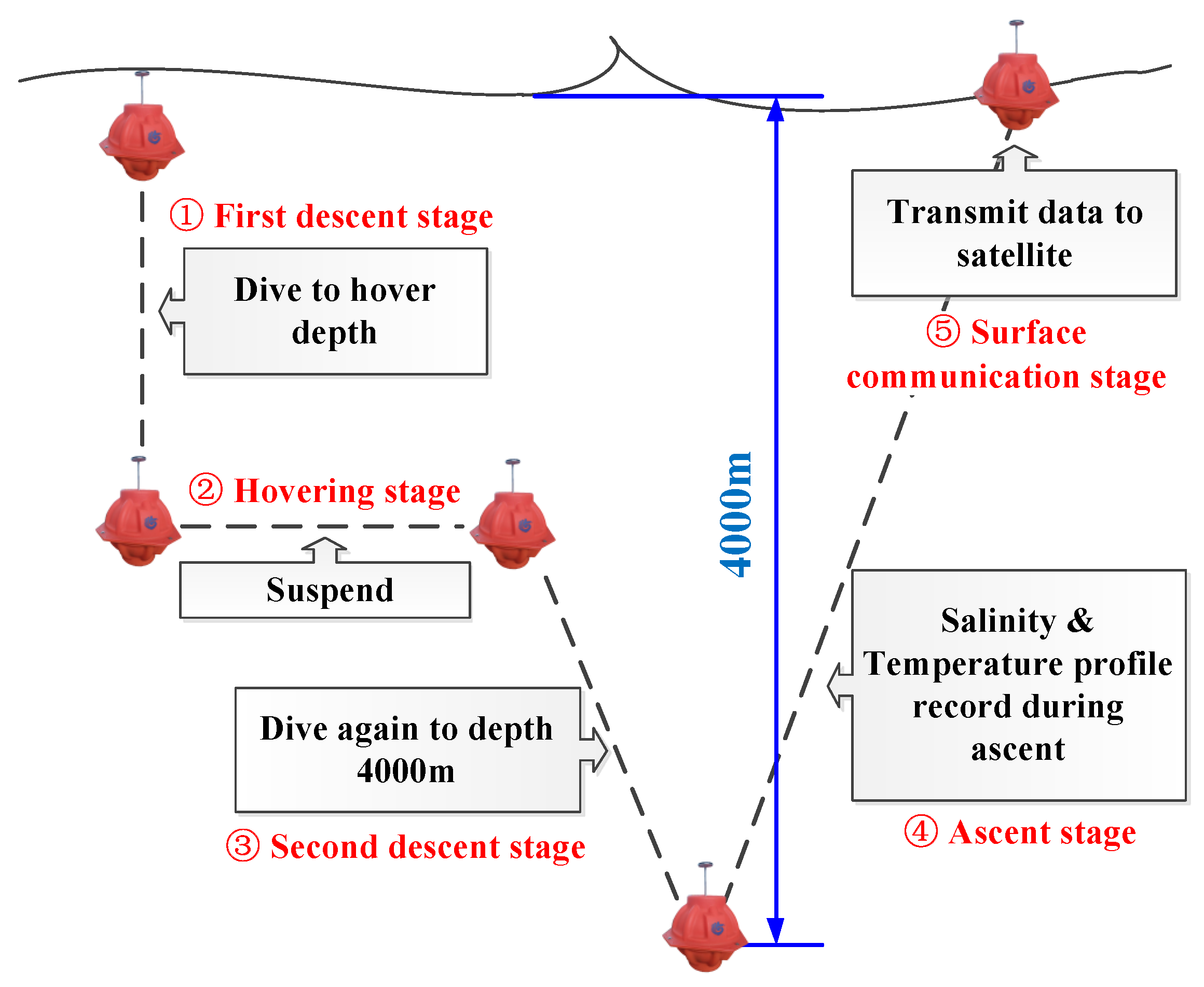
The working process of the DSPB can be divided into: first descent stage, hovering stage, second descent stage, ascent stage and surface communication stage. The specific process is shown in Figure 1 and the running states of devices and sensors of the DSPB are shown in Table 1.
The energy consumption of each working stage indicates that the hovering stage followed by the ascent stage accounts for the highest energy consumption due to long running time compared with remaining stage which is shown in Figure 2.
Reducing the dynamic resistance was not the focus of research in this paper as the design of the DSPB’s shape has been finalized. In addition to the ascent stage, the energy optimization method in other stages are reducing the static energy consumption which is independent of the DSPB’s motion state. As the energy consumption in the ascent stage accounts for a higher proportion, this paper proposes a stage quantitative oil draining control mode to reduce the dynamic energy consumption in the DSPB’s ascent stage. In this mode, the floating speed will definitely decrease resulting in an increase in static energy consumption. Therefore, static energy consumption needs to be considered when establishing the energy consumption optimization model.
2.2. Kinematic Model
The force analysis of the DSPB in the ascent stage is shown in Figure 3.
The gravity of the DSPB is calculated as:
where is the total mass of the DSPB which is 54.53 kg, and g is the gravity acceleration takes 9.8 m/s. The Resistance of the DSPB in ascent stage is expressed as:
is the frictional resistance coefficient of the DSPB which is 0.46 during the ascent stage. S is the DSPB’s total wet area takes 0.77 m after calculate. is the floating speed of the DSPB and t is the floating time. is the density of seawater. The double exponential function and the linear function are used to fit the measured density data of marine experiment at 18.035 N and 114.849 E respectively. The fitting effect is shown in Figure 4 and can be calculated as Formula (3).
There are differences in seawater’s density due to different seasons in different regions. In order to verify the universality of the proposed algorithm, this paper collects seawater’s temperature, salinity and depth data in the southern hemisphere, the equator and the northern hemisphere from the Argo data sharing service platform, and solves the density data through the sea state equation. The double exponential function and polynomial function are used to fit the collected data.
The seawater’s density in the southern hemisphere in summer can be calculated as Formula (4) and data in winter can be expressed as Formula (5) The related parameters are shown in Table 2. The fitting result is shown in Figure 5.
The seawater’s density in the equator area in summer can be calculated as Formula (6) and data in winter can be expressed as Formula (7). The fitting result is shown in Figure 6.
The seawater’s density in the nouthern hemisphere in summer can be calculated as Formula (8) and data in winter can be expressed as Formula (9). The fitting result is shown in Figure 7.
The buoyancy of the DSPB in the ascent stage is calculated as:
is the motor’s oil draining volume which can be expressed as Formula (21). Variety of the DSPB’s body volume is mainly related to two parameters: pressure and temperature of seawater. So the body volume is expressed as:
is the DSPB’s body volume at sea surface which is 0.052884 m. is the body volume variety related to pressure and is body volume variety related to temperature. The pressure at depth 0 m to 4000 m is considered to be varying linearly with depth. Influences of pressure and temperature on the DSPB’s body volume are considered to be linear and can be calculated as:
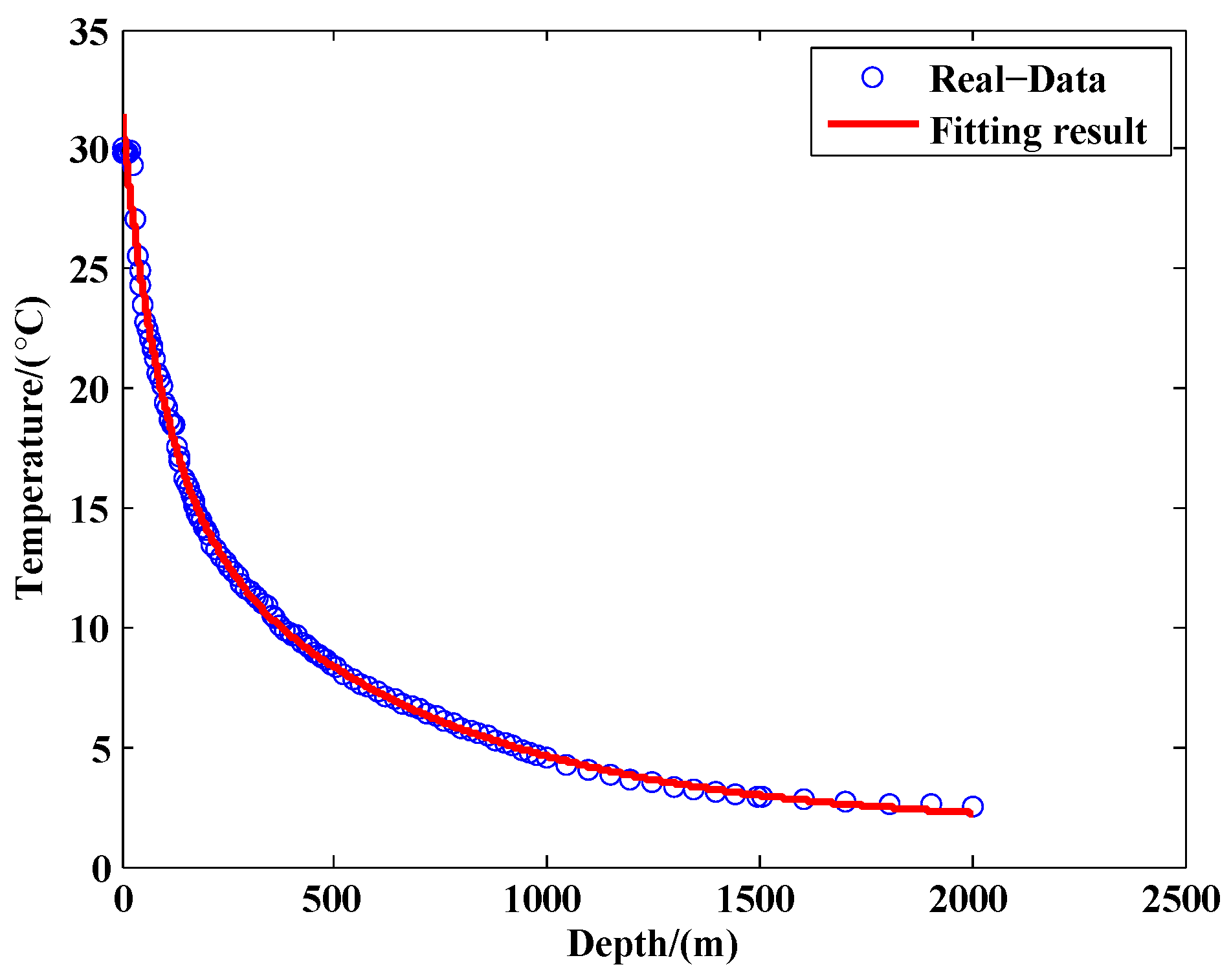
The measured value of marine experiment is used to analyze the temperature changed with depth at 18.035 N and 114.849 E. The temperature at depth of 0 m to 2000 m is fitted using the double exponential function. The temperature at depth of 2000 m to 4000 m can be regarded as a constant. The fitting effect is shown in Figure 8 and can be calculated as Formula (14).
There are differences in seawater’s temperature of different areas and different seasons. In this paper, the temperature data corresponding to the discussed density is fitted by double exponential function and polynomial function.
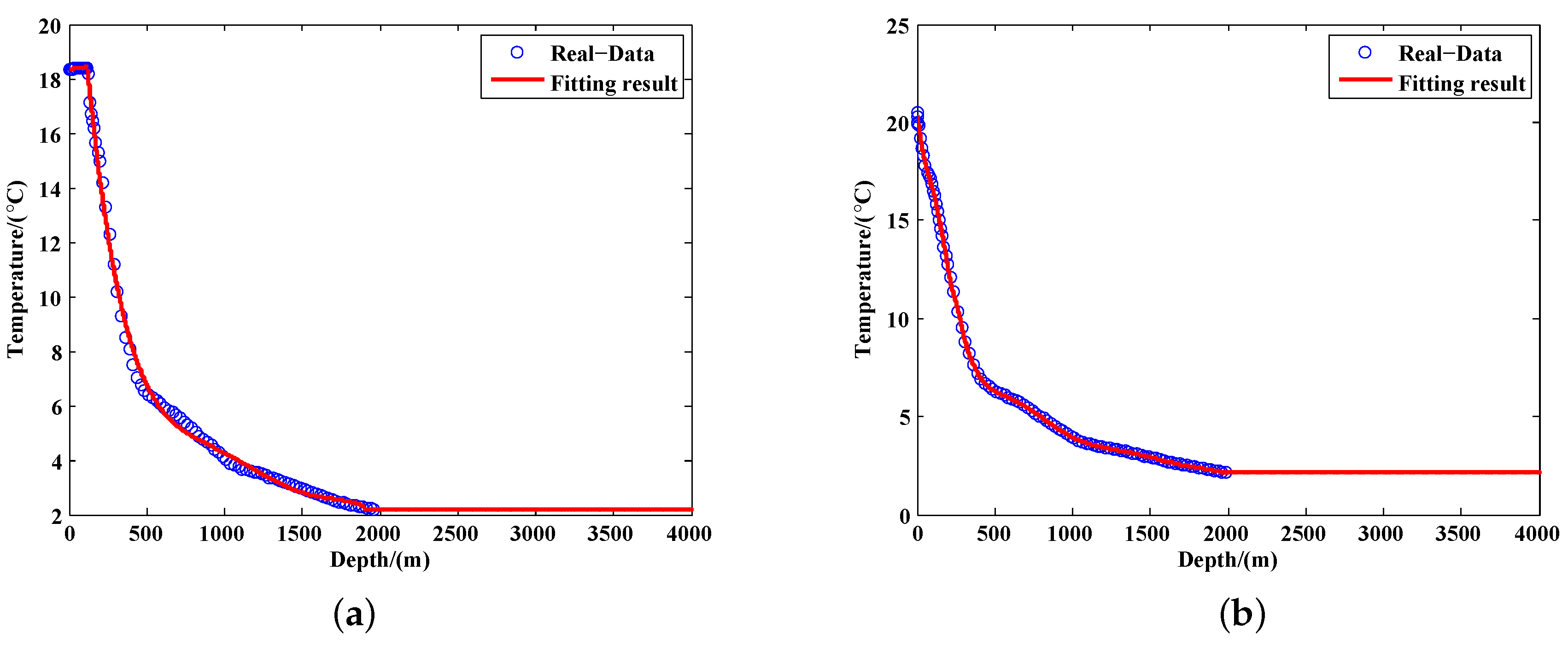
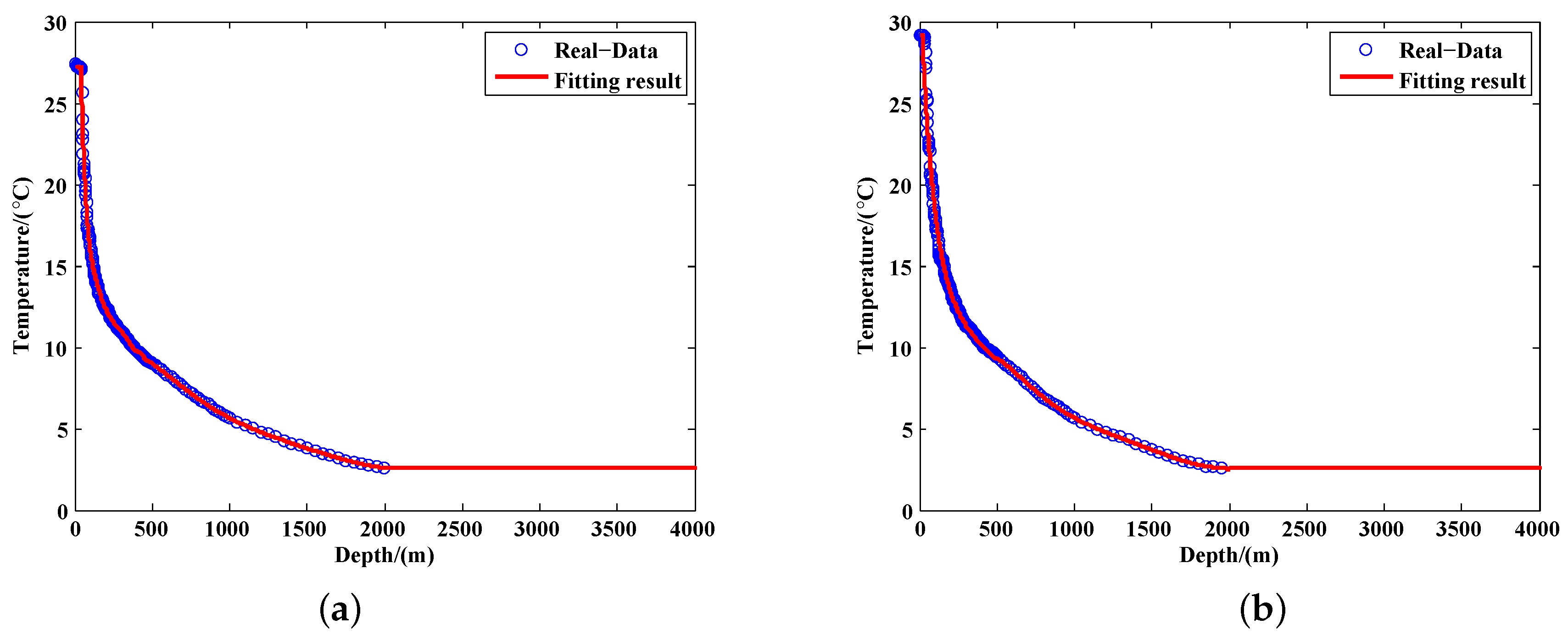
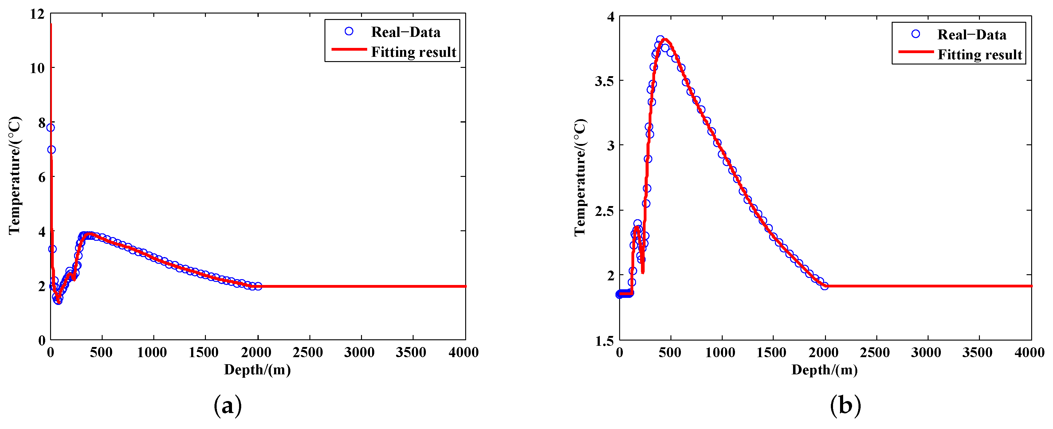
The seawater’s temperature in the southern hemisphere in summer can be calculated as Formula (15) and data in winter can be expressed as Formula (16). The related parameters are shown in Table 3 and Table 4. The fiting result is shown in Figure 9.
The seawater’s temperature in the equator area in summer can be calculated as Formula (17) and data in winter can be expressed as Formula (18). The related parameters are shown in Table 5 and Table 6. The fitting result is shown in Figure 10.
The seawater’s temperature in the northern hemisphere in summer can be calculated as Formula (19) and data in winter can be expressed as Formula (20). The related parameters are shown in Table 7 and Table 8. The fiting result is shown in Figure 11.
The oil draining volume is expressed as:
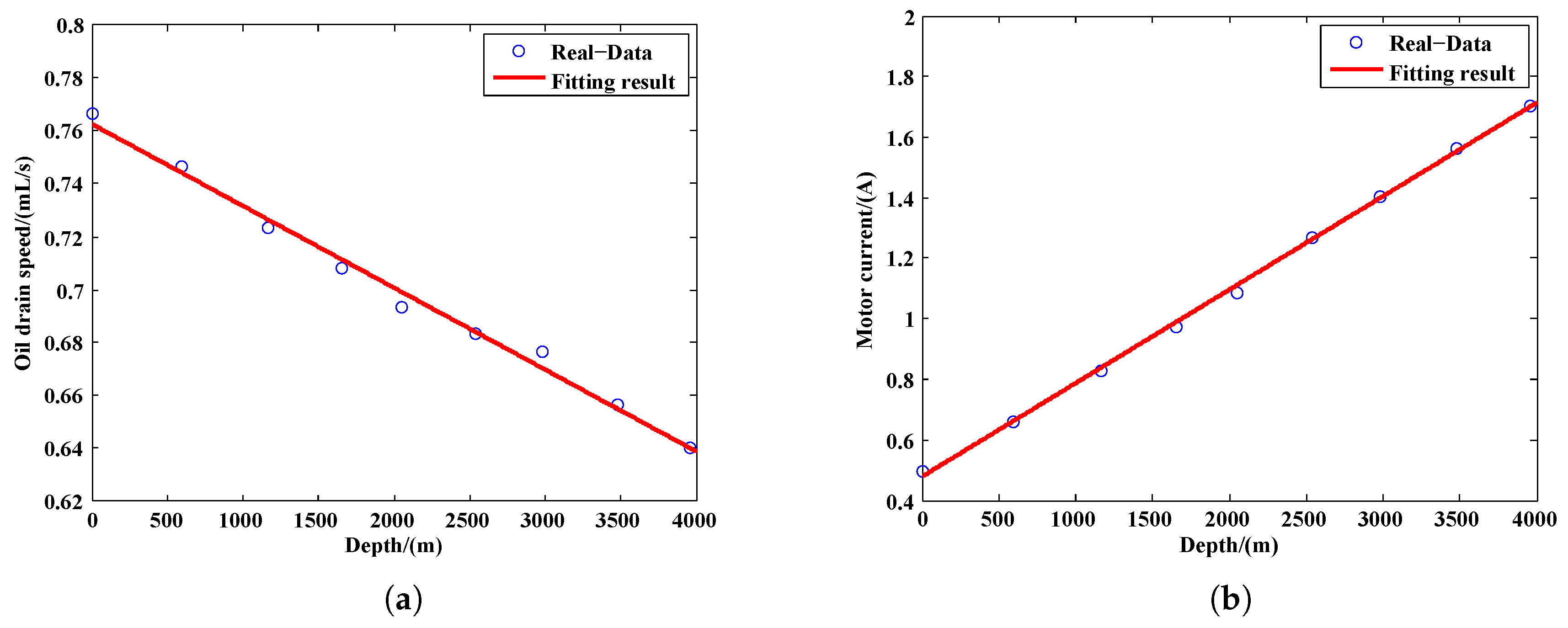
is the time calculation interval of oil draining which takes 1 s. The oil draining speed of the oil pump decreases linearly as the external pressure increases, so the linear function is used to fit the measured data of the oil pump draining speed at 0 to 40 MPa to get the oil pump draining speed varied with depth. The fitting effect is shown in Figure 12a. The oil draining speed is expressed as:
So that the kinematic model of the DSPB can be expressed as:
where is the DSPB’s floating acceleration. is the time calculation interval of ascent stage which takes 1 s. is the DSPB’s floating depth.
2.3. Energy Consumption Model
The energy consumption of the oil pump motor can be calculated as:
The operating voltage of the oil pump motor was set to 28.5 V. The operating current of the oil pump motor increased approximately linearly as the external pressure increased. Therefore, the linear function was used to fit the measured data of the oil pump motor’s operating current at 0 to 40MPa. The fitting effect is shown in Figure 12b. The operating current of the oil pump motor can be calculated as:
The static energy consumption of the DSPB in the ascent stage is expressed as:
and are operating voltage of the control board and the CTD sensor. They are set to 28.5 V and 12 V respectively. The operating current of the control board and the CTD sensor are and which are setting to 0.010346A and 0.018998A in average value.
2.4. Stage Quantitative Oil Draining Control Model
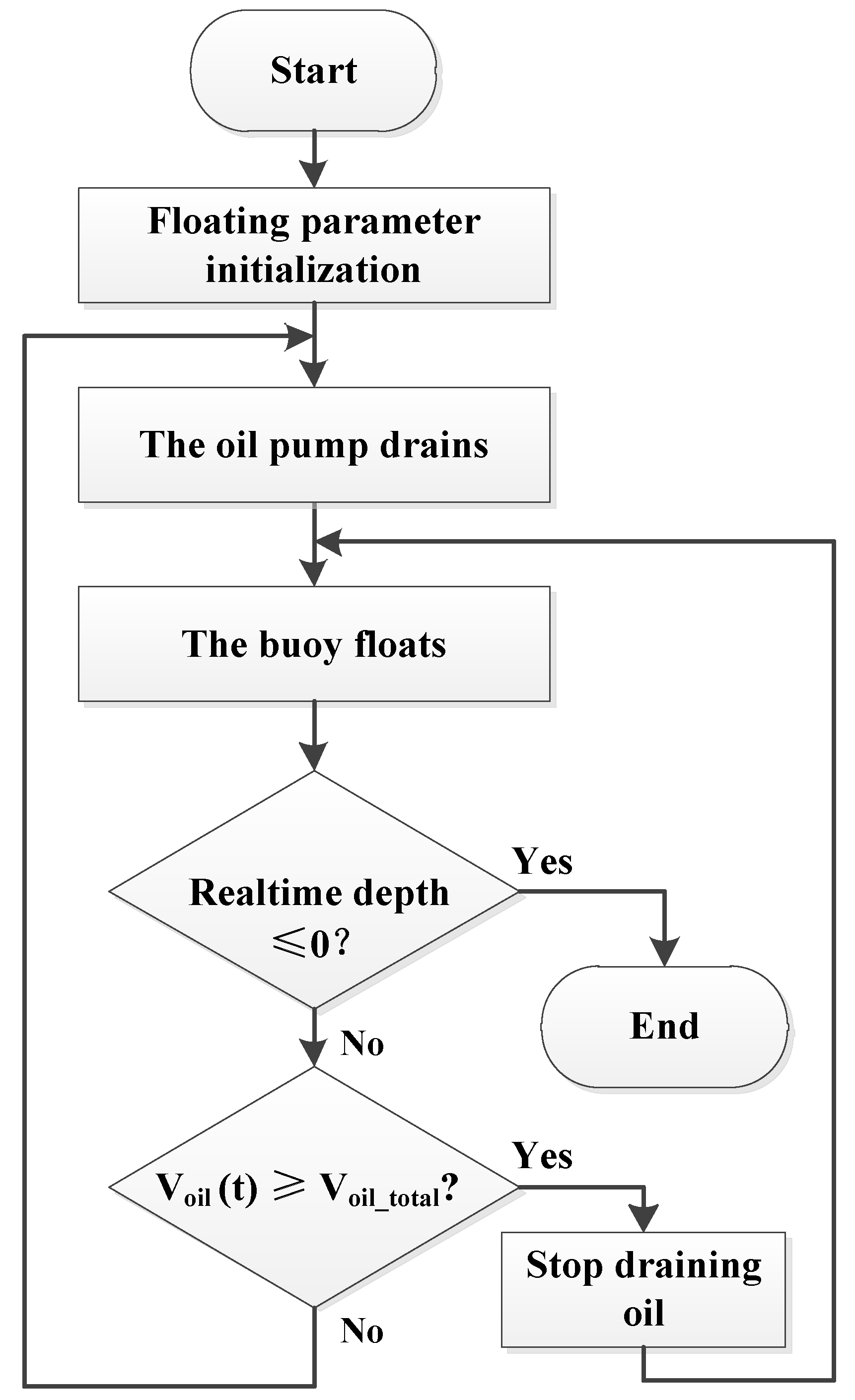
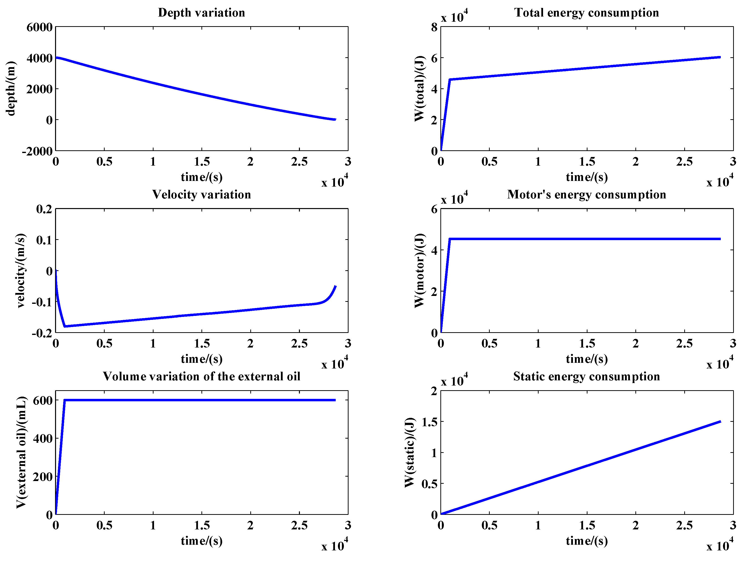
Before optimization, the oil draining method of the ascent stage was one-time oil draining which is shown in Figure 13, and parameters of the ascent stage are shown in Figure 14. The oil draining process was carried out in the deeper sea area where the external resistance of the oil pump motor is relatively larger than shallow sea area, resulting in the larger working current of the motor, and the oil draining speed is slower which can be seen from Figure 12. In this scheme, the working efficiency of the motor was lower and the energy consumption is higher.
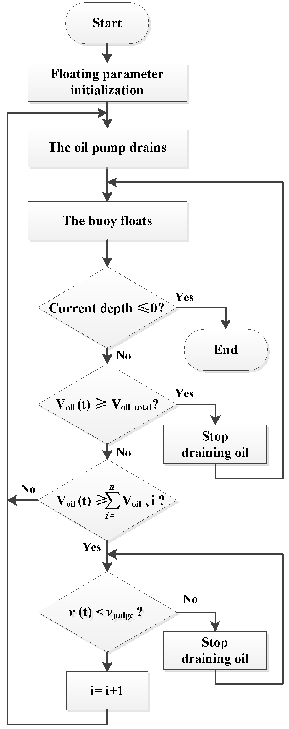
In order to optimize the oil draining mode of the oil pump motor during the DSPB’s ascent stage, a stage quantitative oil draining control mode is established which is shown in Figure 15. The stage quantitative oil draining control mode will indeed reduce the dynamic energy consumption but the static energy consumption will increase as the DSPB’s floating speed will rev down. So the energy consumption model was established by considering the increase of the static energy consumption.
2.5. Energy Consumption Model
2.5.1. Single-Objective Model
Objective function:
Decision variables:
is the stage oil draining volume expressed as an n-dimensional row vector, n indicates the total frequency of oil draining, and is the judgment threshold of the floating speed to decide whether to carry out the next oil draining.
2.5.2. Multi-Objective Model
The setting of in the single-objective optimization model led to the optimization result being limited to the hardware design. The improvement of the design of the hardware will lead to the further reduction of the static working current of the control board, then the single-objective optimization model needed to adjust the static energy consumption parameters to adapt to the change of the static working current.
The stage quantitative oil draining control mode will only increases the floating time t, and does not affect the static working current of the control board and CTD sensor. Therefore, a multi-objective optimization model is established to enhance the applicability of the energy optimization model taking and floating time t as optimization targets.
Objective functions:
Decision variables are same to the single-objective model.
2.6. NSGA-II Method
Since 1950, scientists have come up with the idea of using genetic algorithms to solve engineering problems. At first, it has good convergence and robustness prototype by biological evolution, and it takes less time to calculate accuracy [52]. The non-dominated sorted genetic algorithm (NSGA) is a multi-objective optimization algorithm based on genetic algorithm but has disadvantages in some aspects introduced in [53]. An improved version of NSGA call NSGA-II is proposed by Deb et al. which reduces the computational complexity with a fast non-dominated sorting algorithm. The elite strategy ensures that the excellent individuals will be reserved during the evolution process, thereby improving the accuracy of the optimization results. The congestion comparison operator ensures the diversity of the population. The optimization process of NSGA-II method is shown in Figure 16.
3. Results and Discussion
The first section of this chapter will analyze the result of single-objective model optimization, the second section will verify the accuracy and timeliness of the NSGA-II method by traversing method, and the third section will analyze the result of single-objective model optimization and give the optimized effect compared with pre-optimization.
Test hardware: CPU: Intel(R) Core(TM) i3-3227U; RAM: 4 G. The operating system was Windows 7—64 bit and the simulation software was Matlab R2014a.
3.1. Single-Objective Model Optimization
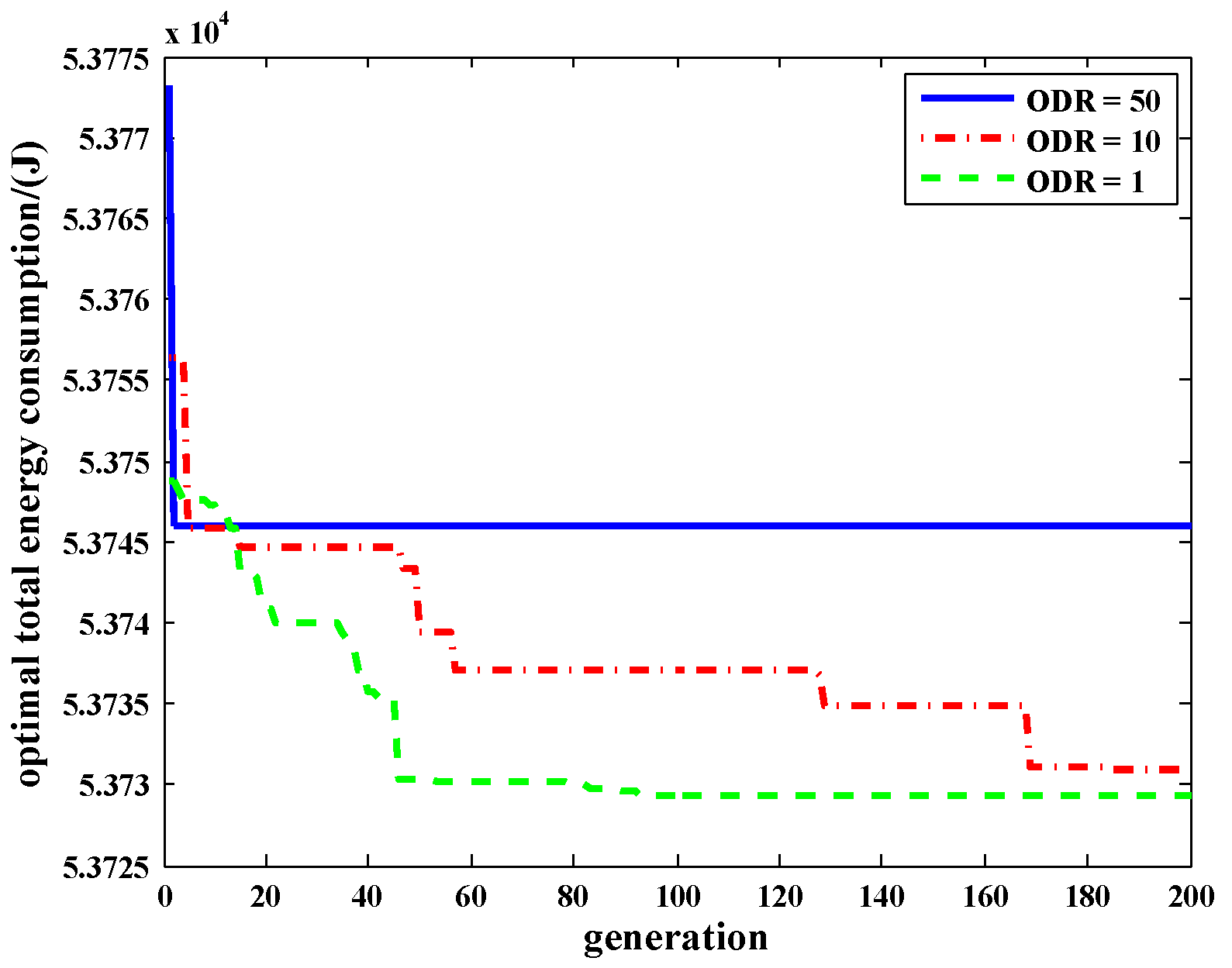
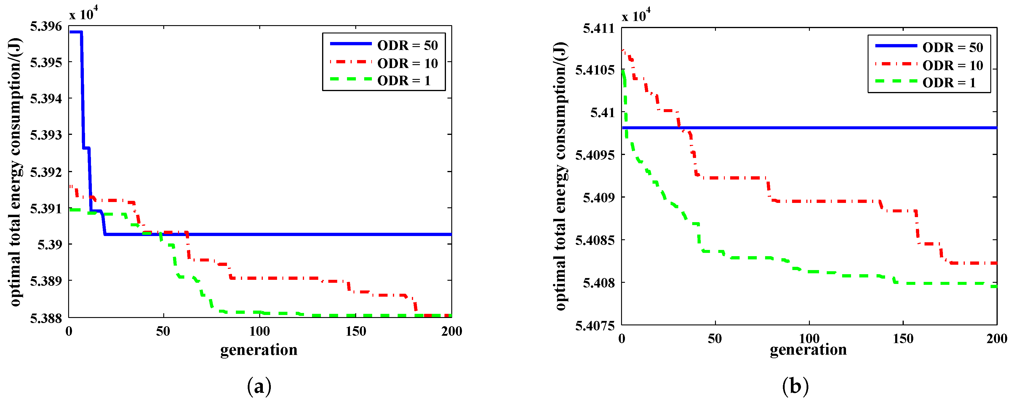
In order to ensure that the DSPB floats from depth 4000m to the surface to complete normal communication, the total oil draining amount was set to 600 mL. The NSGA-II method is used to optimize the single-objective energy consumption model. Parameters of proposed NSGA-II method is shown in Table 9. The ODR was set to 50 mL, 10 mL, 1 mL respectively to get the optimized results shown in Figure 17.
Figure 17 shows that when ODR=10 mL, the optimal energy consumption will be further reduced compared with ODR = 50 mL. However, the advantage of ODR = 1 mL compared with ODR = 10 mL was not obvious. Taking into account the oil quantity error generated when the oil pump is turned on and off and the measurement error existing in the oil quantity measurement, the ODR was more suitable for 10 mL.
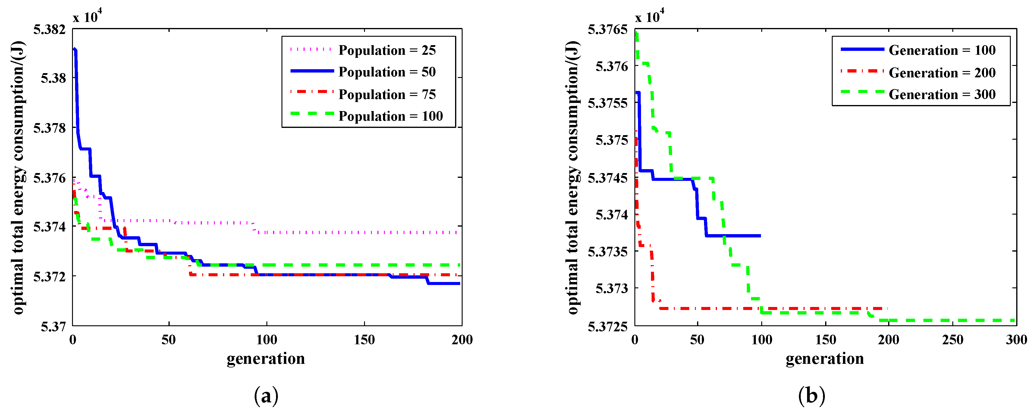
In order to evaluate the parameters set by NSGA-II, this paper compares the optimal results by changing population number and evolution algebra parameters. The optimal results are shown in the Figure 18 and the optimization time of them are shown in Table 10. The results show that after more than 50 populations, the optimization effect was not significantly improved, but the running time did increased. After more than 200 generations of evolutionary algebra, the optimization results remain basically stable, and increasing the evolutionary algebra will increase the time cost to a large extent.
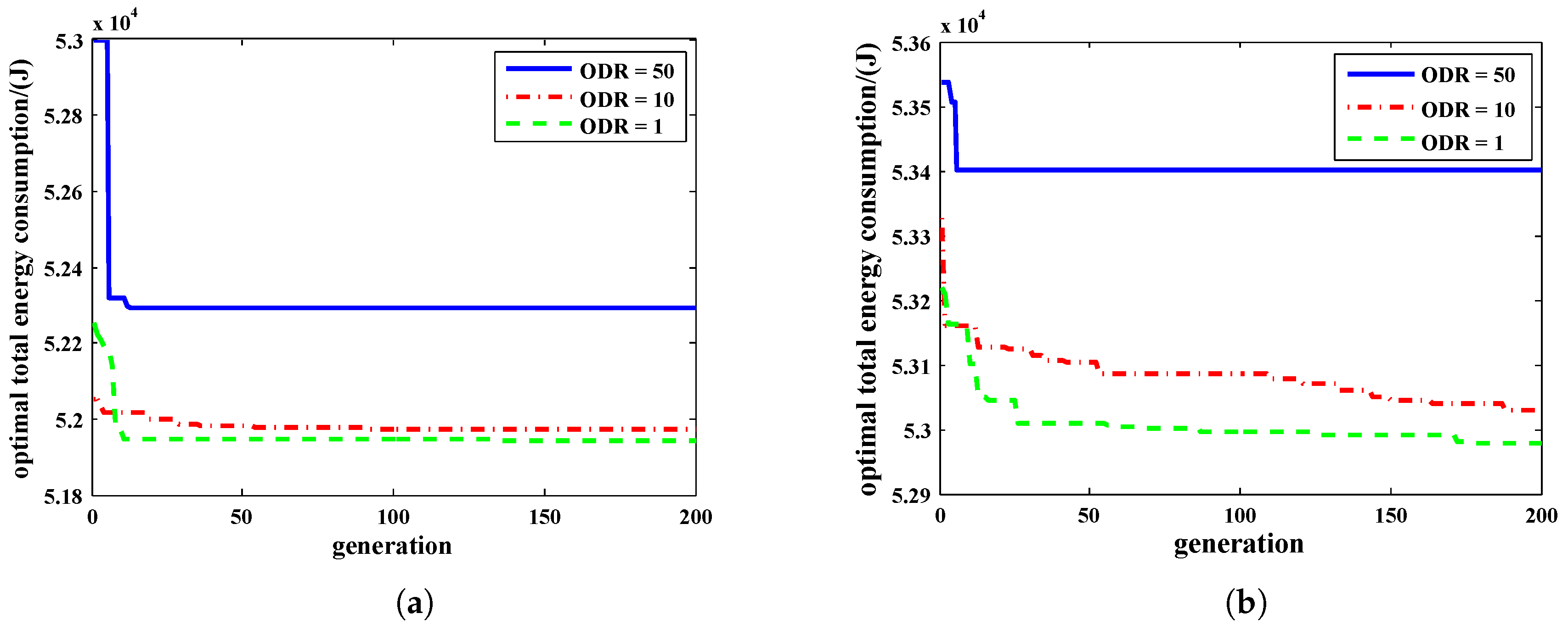
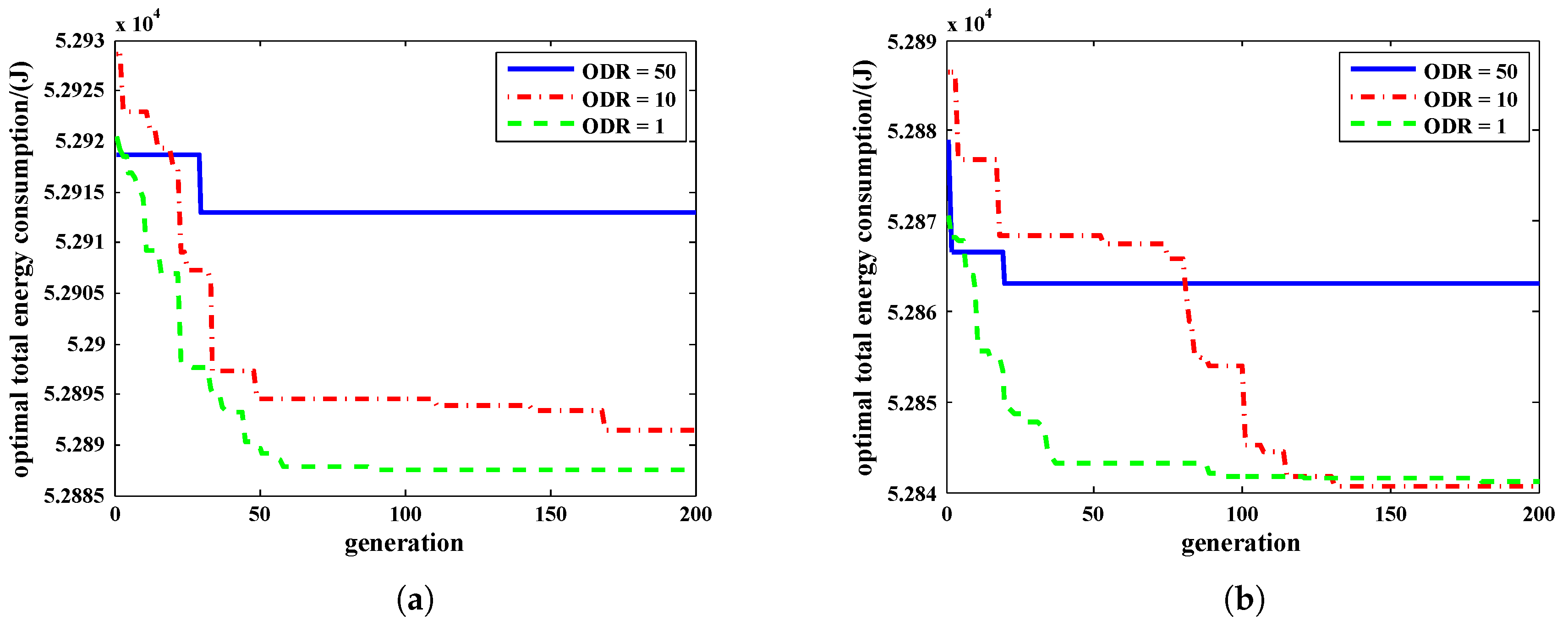
The DSPB’s kinematics models for different seasons in different regions are optimized by the NSGA-II method proposed in this paper. Optimization results are shown in the Figure 19, Figure 20 and Figure 21. The results show that the proposed NSGA-II method can be applied to the optimization of DSPB’s energy consumption in different regions and different seasons.
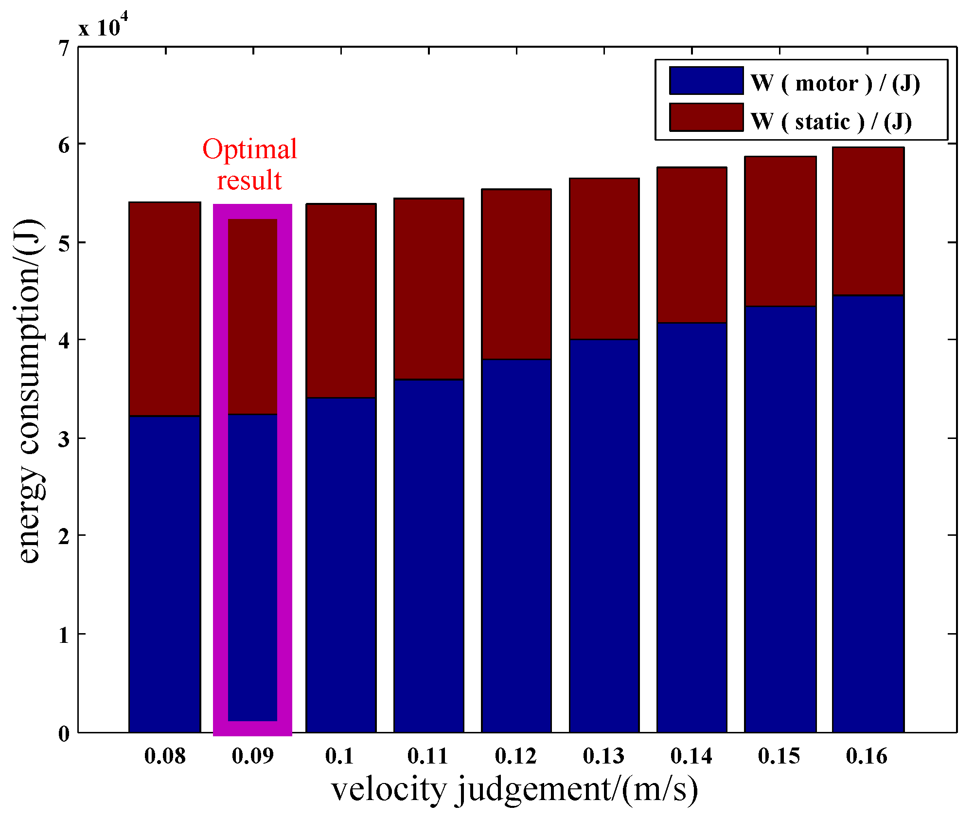
3.2. Traversal Single-Objective Model Optimization
In order to verify the accuracy and timeliness of the NSGA-II method, the traversal method is adopted with the ODR setting to 50 mL to analyze the measured data of the ocean experiment at 18.035 N and 114.849 E in August 2018. After 18,433 combinations traversed, the minimum energy consumption of different velocity judgment is shown in Figure 22. The traversing time is about 4 h and will increase to more than several weeks if the ODR is improved to 10 mL. After 10 repetitions, the optimization result of the NSGA-II method is shown in Table 11. The traversing time of the NSGA-II method is changed by the set of maximum generation. After repeating the simulation, the traversing time is less than 6 min within 10 generations when the ODR is set to 50 mL. As the maximum generation is set to 200 in this paper, the average optimization time of the NSGA-II method is about 1.99 h with satisfactory results when ODR is set to 10 mL.
3.3. Multi-Objective Model Optimization
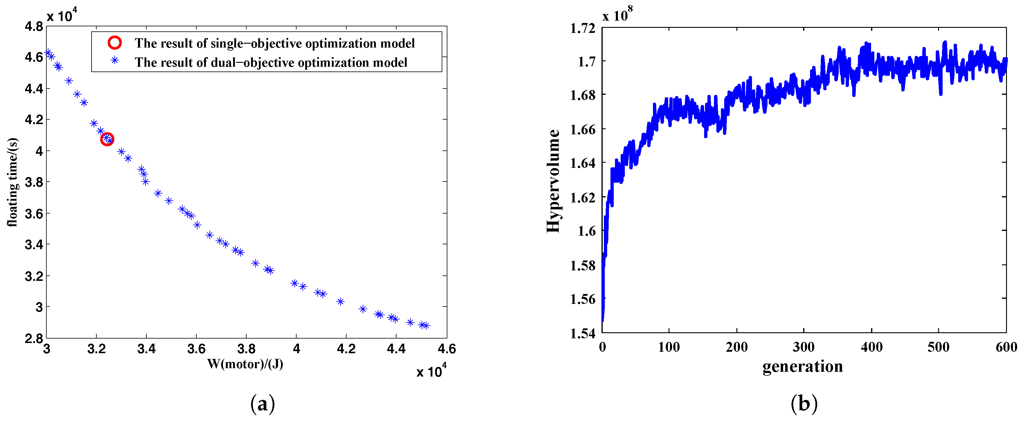
The NSGA-II method is good at solving multi-objective problems and the Pareto optimization results are shown in Figure 23a with the ODR set to 10 mL and other parameters of NSGA-II algorithm are shown in Table 12. The hypervolume value [54,55,56] computed by means of Monte-Carlo approximation method is shown in Figure 23b to evaluate the convergence and distribution of the solution. The variety of the hypervolume value shows that the solution tends to converge after 400 generations.
Figure 23 shows that the multi-objective optimization model established in this paper can be optimized by the NSGA-II method, and the optimal solution can be selected according to different static energy consumption.
4. Conclusions
The energy consumption of the DSPB’s whole working stage has been analyzed in this paper. A single-objective energy optimization model and a multi-objective energy optimization model have been established by combining the kinematics model of the DSPB’s ascent stage. The NSGA-II method has been applied to optimize these energy consumption optimization models. The ODR has been analyzed taking into account the error caused by shutting down the oil pump and the oil measurement. The main conclusions are summarized as follows:
- (1)
- On the basis of considering the static energy consumption will change in the floating stage, the stage quantitative oil draining control mode can replace the one-time oil draining mode as an optimization scheme for the DSPB’s ascent stage.
- (2)
- Using traversal method and the NSGA-II method for comparative analysis, the NSGA-II method as the energy consumption optimization of the DSPB have been determined. The accuracy and timeliness of the NSGA-II method have been verified.
- (3)
- The advantage of the ODR set to 1 mL is not obvious compared with 10 mL. When the ODR is set to 1 mL, the control accuracy of the oil pump is difficult to achieve, so it is appropriate to set the ODR to 10 mL. In this case, the optimized judgment threshold of the floating speed is 0.09 m/s, and the optimal frequency of oil draining is 10 times contains 160 mL, 30 mL, 30 mL, 40 mL, 50 mL, 50 mL, 60 mL, 70 mL, 80 mL, 30 mL respectively.
- (4)
- The static working current of the DSPB in this paper is about 10 mA, and this parameter can be further optimized. A set of Pareto solutions for the ascent stage have been obtained in the multi-objective optimization model with the dynamic energy consumption of the oil pump motor and the floating time as objective functions, so that the appropriate oil draining mode can be selected according to different static energy consumption.
In the future work, we will further optimize the energy consumption according to the working mode of the DSPB and further reduce it’s static energy consumption. The algorithm proposed in this paper will be further improved and other better genetic algorithm will be adopted [57,58]. The optimization effect of the optimization scheme in this paper will be verified in the following ocean experiments.
Author Contributions
Conceptualization, X.L. and H.L.; methodology, M.L.; software, M.L.; validation, M.L. and J.X.; formal analysis, M.L.; investigation, M.L.; resources, X.L., S.Y. and H.L.; data curation, M.L., X.L. and H.L.; writing–original draft preparation, M.L.; writing–review and editing, M.L., J.X., S.Y. and X.L.; visualization, M.L.; supervision, X.L. and H.L.; project administration, X.L. and H.L.; funding acquisition, X.L.
Funding
This research was funded by “National Natural Science Foundation of China” and the grant number is 61733012.
Acknowledgments
“Qingdao National Labboratory for Marine Science and Technology” provided materials used for experiments and the project number is ’ZR2016WH01’. Yanlong Zhao provided help for the experiment. Meiqi Fang provided help for the kinematics model establishment.
Conflicts of Interest
The authors declare no conflict of interest.
Nomenclature
| time interval of ascent stage, s | |
| time interval of oil drain, s | |
| volume change related to pressure, m | |
| volume change related to temperature, m | |
| seawater density, kg/m | |
| a | acceleration, m/s |
| frictional resistance coefficient | |
| buoyancy, N | |
| resistance, N | |
| g | gravity acceleration, m/s |
| h | floating depth, m |
| operating current of the control board, A | |
| operating current of the CTD sensor, A | |
| operating current of the oil pump motor, A | |
| m | mass, kg |
| S | total wet area of the DISB, m |
| t | floating time, s |
| seawater temperature, °C | |
| operating voltage of the control board, V | |
| operating voltage of the CTD sensor, V | |
| operating voltage of the oil pump motor, V | |
| v | floating speed, m/s |
| body volume, m | |
| judgment threshold of the floating speed, m/s | |
| oil drain speed, m/s | |
| stage oil drain volume, m | |
| oil drain volume, m | |
| energy consumption of oil pump motor, J | |
| static energy consumption, J | |
| total energy consumption of ascent process, J |
Abbreviations
The following abbreviations are used in this manuscript:
| DSPB | deep-sea self-sustaining profile buoy |
| ODR | oil discharge resolution |
| NSGA-II | non-dominated sorted genetic algorithm-II |
References
- Gould, J.; Roemmich, D.; Wijffels, S.; Freeland, H.; Ignazewsky, M.; Jianping, X.; Pouliquen, S.; Desaubies, Y.; Send, U.; Radhakrishnan, K.; et al. Argo profiling floats bring new era of in situ ocean observations. Eos Trans. Am. Geophys. Union 2013, 85, 185–191. [Google Scholar] [CrossRef]
- Freeland, H.J.; Cummins, P.F. Argo: A new tool for environmental monitoring and assessment of the world’s oceans, an example from the N.E. Pacific. Prog. Oceanogr. 2005, 64, 31–44. [Google Scholar] [CrossRef]
- Roemmich, D.H.; Davis, R.E.; Riser, S.C. The ARGO Project: Global Ocean Observations for Understanding and Prediction of Climate Variability. Report for Calendar Year 2004. Oceanography 2000, 7, 45–50. [Google Scholar] [CrossRef]
- Zhu, X.; Yu, J.; Wang, X. Sampling Path Planning of Underwater Glider for Optimal Energy Consumption. Robot 2011, 33, 360–365. [Google Scholar] [CrossRef]
- Wang, S.; Jin, H.; Meng, L.; Li, G. Optimize motion energy of AUV based on LQR control strategy. In Proceedings of the 2016 35th Chinese Control Conference (CCC), Chengdu, China, 27–29 July 2016; pp. 27–29. [Google Scholar]
- Sun, C.; Song, B.; Wang, P.; Zhang, B. Energy consumption optimization of steady-state gliding for a Blended-Wing-Body underwater glider. In Proceedings of the OCEANS 2016 MTS/IEEE Monterey, Monterey, CA, USA, 19–23 September 2016; pp. 19–23. [Google Scholar]
- Giron-Sierra, J.M.; Fernandez-Prisuelos, J.; Andres-Toro, B.; de la Cruz, J.M. A multiobjective optimization issue: Genetic control planning for AUV trajectories. In Proceedings of the 7th WSEAS International Conference on Automatic Control, Modeling and Simulation, Prague, Czech Republic, 13–15 March 2005. [Google Scholar]
- Koh, H.J.; Ruy, W.S.; Cho, I.H.; Kweon, H.M. Multi-objective optimum design of a buoy for the resonant-type wave energy converter. J. Mar. Sci. Technol. 2015, 20, 53–63. [Google Scholar] [CrossRef]
- Liu, T.; Gao, X.; Wang, L. Multi-objective optimization method using an improved NSGA-II algorithm for oil–gas production process. J. Taiwan Inst. Chem. Eng. 2015, 57, 42–53. [Google Scholar] [CrossRef]
- Alikar, N.; Mousavi, S.M.; Ghazilla, R.A.R.; Tavana, M.; Olugu, E.U. Application of the NSGA-II algorithm to a Multi-Period Inventory-Redundancy Allocation Problem in a Series-Parallel System. Reliab. Eng. Syst. Saf. 2017, 160, 1–10. [Google Scholar] [CrossRef]
- Bedatri, M.; Dirk, S. Optimal Rule-Based Power Management for Online, Real-Time Applications in HEVs with Multiple Sources and Objectives: A Review. Energies 2015, 8, 9049–9063. [Google Scholar] [Green Version]
- Nath, R.; Shukla, A.K.; Muhuri, P.K.; Lohani, Q.M.D. NSGA-II based energy efficient scheduling in real-time embedded systems for tasks with deadlines and execution times as type-2 fuzzy numbers. In Proceedings of the IEEE International Conference on Fuzzy Systems, Hyderabad, India, 7–10 July 2013; pp. 7–10. [Google Scholar]
- Ming, M.; Wang, R.; Zha, Y.; Zhang, T. Multi-Objective Optimization of Hybrid Renewable Energy System Using an Enhanced Multi-Objective Evolutionary Algorithm. Energies 2017, 10, 674. [Google Scholar] [CrossRef]
- Luceny, G.A.; Maree, L.; Ricardo, V.P.; Yee, Y.L.; Esneyder, G.P.; Yen, C.S.T. Modelling autonomous hybrid photovoltaic-wind energy systems under a new reliability approach. Energy Convers. Manag. 2018, 172, 357–369. [Google Scholar]
- Kong, D.S.; Jang, Y.S.; Huh, J.H. Method and Case Study of Multiobjective Optimization-Based Energy System Design to Minimize the Primary Energy Use and Initial Investment Cost. Energies 2015, 8, 6114–6134. [Google Scholar] [CrossRef] [Green Version]
- Wang, H.; He, C.; Liu, Y. Pareto Optimization of Power System Reconstruction Using NSGA-II Algorithm. In Proceedings of the 2010 Asia-Pacific Power and Energy Engineering Conference, Chengdu, China, 28–31 March 2010; pp. 28–31. [Google Scholar]
- Hu, Y.; Bie, Z.; Ding, T.; Lin, Y. An NSGA-II based multi-objective optimization for combined gas and electricity network expansion planning. Appl. Energy 2015, 167, 280–293. [Google Scholar] [CrossRef]
- Kannan, S.; Baskar, S.; Mccalley, J.; Murugan, P. Application of NSGA-II Algorithm to Generation Expansion Planning. IEEE Trans. Power Syst. 2009, 24, 454–461. [Google Scholar] [CrossRef]
- Murugan, P.; Kannan, S.; Baskar, S. Application of NSGA-II Algorithm to Single-Objective Transmission Constrained Generation Expansion Planning. IEEE Trans. Power Syst. 2009, 24, 1790–1797. [Google Scholar] [CrossRef]
- Sadatsakkak, S.A.; Ahmadi, M.H.; Ahmadi, M.A. Optimization performance and thermodynamic analysis of an irreversible nano scale Brayton cycle operating with Maxwell–Boltzmann gas. Energy Convers. Manag. 2015, 101, 592–605. [Google Scholar] [CrossRef]
- Basu, M. Fuel constrained economic emission dispatch using nondominated sorting genetic algorithm-II. Energy 2014, 78, 649–664. [Google Scholar] [CrossRef]
- Cao, K.; Batty, M.; Huang, B.; Liu, Y.; Yu, L.; Chen, J. Spatial multi-objective land use optimization: extensions to the non-dominated sorting genetic algorithm-II. Int. J. Geograph. Inf. Sci. 2011, 25, 1949–1969. [Google Scholar] [CrossRef]
- Shiri, A.; Shoulaie, A. End effect braking force reduction in high-speed single-sided linear induction machine. Energy Convers. Manag. 2012, 61, 43–50. [Google Scholar] [CrossRef]
- Lotfan, S.; Ghiasi, R.A.; Fallah, M.; Sadeghi, M.H. ANN-based modeling and reducing dual-fuel engine’s challenging emissions by multi-objective evolutionary algorithm NSGA-II. Appl. Energy 2016, 175, 91–99. [Google Scholar] [CrossRef]
- Krzysztof, G.; Joanna, F.G. Multi-Objective Optimization of the Envelope of Building with Natural Ventilation. Energies 2018, 11, 1383. [Google Scholar] [Green Version]
- Panda, S. Multi-objective PID controller tuning for a FACTS-based damping stabilizer using Non-dominated Sorting Genetic Algorithm-II. Int. J. Electr. Power Energy Syst. 2011, 33, 1296–1308. [Google Scholar] [CrossRef]
- Zhong, H.H.; Zhong, K.M.; Peng, L. Multi-objective optimization and sensitivity analysis of an organic Rankine cycle coupled with a one-dimensional radial-inflow turbine efficiency prediction model. Energy Convers. Manag. 2018, 166, 37–47. [Google Scholar]
- Reed, P.; Minsker, B.S.; Goldberg, D.E. Simplifying multiobjective optimization: An automated design methodology for the nondominated sorted genetic algorithm-II. Water Resour. Res. 2003, 39, 1196. [Google Scholar] [CrossRef]
- Tomoiagă, B.; Chindriş, M.; Sumper, A.; Sudria-Andreu, A.; Villafafila-Robles, R. Pareto Optimal Reconfiguration of Power Distribution Systems Using a Genetic Algorithm Based on NSGA-II. Energies 2013, 6, 1439–1455. [Google Scholar] [CrossRef] [Green Version]
- Lakshminarasimman, N.; Baskar, S.; Alphones, A.; Willjuice, I.M. Evolutionary multiobjective optimization of cellular base station locations using modified NSGA-II. Wirel. Netw. 2011, 17, 597–609. [Google Scholar] [CrossRef]
- Frutos, M.; Olivera, A.C.; Tohmé, F. A memetic algorithm based on a NSGA-II scheme for the flexible job-shop scheduling problem. Annal. Operat. Res. 2010, 181, 745–765. [Google Scholar] [CrossRef]
- Agrawal, N.; Rangaiah, G.P.; Ray, A.K.; Gupta, S.K. Design stage optimization of an industrial low-density polyethylene tubular reactor for multiple objectives using NSGA-II and its jumping gene adaptations. Chem. Eng. Sci. 2007, 62, 2346–2365. [Google Scholar] [CrossRef]
- Gopal, N.R.; Satyanarayana, S.V. Cost analysis for removal of VOCs from water by pervaporation using NSGA-II. Desalination 2011, 274, 212–219. [Google Scholar] [CrossRef]
- Ye, C.J.; Huang, M.X. Multi-Objective Optimal Power Flow Considering Transient Stability Based on Parallel NSGA-II. IEEE Trans. Power Syst. 2015, 30, 857–866. [Google Scholar] [CrossRef]
- Agarwal, A.; Gupta, S.K. Jumping gene adaptations of NSGA-II and their use in the multi-objective optimal design of shell and tube heat exchangers. Chem. Eng. Res. Des. 2008, 86, 123–139. [Google Scholar] [CrossRef]
- Bekele, E.G.; Nicklow, J.W. Multi-objective automatic calibration of SWAT using NSGA-II. J. Hydrol. 2007, 341, 165–176. [Google Scholar] [CrossRef]
- Nemmani, G.R.; Suggala, S.V.; Bhattacharya, P.K. NSGA-II for Multiobjective Optimization of Pervaporation Process: Removal of Volatile Organics from Water. Ind. Eng. Chem. Res. 2009, 48, 1543–1550. [Google Scholar] [CrossRef]
- Majumdar, S.; Mitra, K.; Raha, S. Optimized species growth in epoxy polymerization with real-coded NSGA-II. Polymer 2005, 46, 11858–11869. [Google Scholar] [CrossRef]
- Li, Y.; Lu, X.; Kar, N.C. Rule-Based Control Strategy With Novel Parameters Optimization Using NSGA-II for Power-Split PHEV Operation Cost Minimization. IEEE Trans. Veh. Technol. 2014, 63, 3051–3061. [Google Scholar] [CrossRef]
- Sharma, N.; Anupama, K.R. On the use of NSGA-II for multi-objective resource allocation in MIMO-OFDMA systems. Wirel. Netw. 2011, 17, 1191–1201. [Google Scholar] [CrossRef]
- Ghorbani, B.; Shirmohammadi, R.; Mehrpooya, M. Structural, operational and economic optimization of cryogenicnatural gas plant using NSGA-II two-objective genetic algorithm. Energy 2018, 159, 410–428. [Google Scholar] [CrossRef]
- Li, M.; Lin, D.; Wang, S. Solving a type of biobjective bilevel programming problem using NSGA-II. Comput. Math. Appl. 2010, 59, 706–715. [Google Scholar] [CrossRef]
- Katiani, P.; Rodrigues, P.J.B.; Javier, C.; Roberto, S.M.J. A Multi-Objective Optimization Technique to Develop Protection Systems of Distribution Networks with Distributed Generation. IEEE Trans. Power Syst. 2018, 33, 7064–7075. [Google Scholar]
- Dai, C.; Qin, X.S.; Chen, Y.; Guo, H.C. Dealing with equality and benefit for water allocation in a lake watershed: A Gini-coefficient based stochastic optimization approach. J. Hydrol. 2018, 561, 322–334. [Google Scholar] [CrossRef]
- Cavalcante, M.A.; Pereira, H.A.; Chaves, D.A.R.; Almeida, R.C. Evolutionary Multiobjective Strategy for Regenerator Placement in Elastic Optical Networks. IEEE Trans. Commun. 2018, 66, 3583–3596. [Google Scholar] [CrossRef]
- Muhuri, P.K.; Ashraf, Z.; Lohani, Q.M.D. Multi-objective Reliability-Redundancy Allocation Problem with Interval Type-2 Fuzzy Uncertainty. IEEE Trans. Fuzzy Syst. 2018, 26, 1339–1355. [Google Scholar] [CrossRef]
- Cheraghchi, F.; Abualhaol, I.; Falcon, R.; Abielmona, R.; Raahemi, B.; Petriu, E. Modeling the Speed-based Vessel Schedule Recovery Problem using Evolutionary Multiobjective Optimization. Inf. Sci. 2018, 448–449, 53–74. [Google Scholar] [CrossRef]
- Paul, A.K.; Shill, P.C. New Automatic Fuzzy Relational Clustering Algorithms Using Multi-Objective NSGA-II. Inf. Sci. 2018, 448–449, 112–133. [Google Scholar] [CrossRef]
- Zhu, J.Y.; Li, C.; Bin, W.; Xia, L. Optimal design of a hybrid electric propulsive system for an anchor handling tug supply vessel. Appl. Energy 2018, 226, 423–436. [Google Scholar] [CrossRef]
- Wang, C.Y.; Li, Y.; Zhao, W.Z.; Zou, S.C.; Zhou, G.; Wang, Y.L. Structure design and multi-objective optimization of a novel crash box based on biomimetic structure. Int. J. Mech. Sci. 2018, 138–139, 489–501. [Google Scholar] [CrossRef]
- Lotfi, R.A.; Beyranvand, H.; Salehi, J.A.; Maier, M. Ultra-Dense 5G Small Cell Deployment for Fiber and Wireless Backhaul-Aware Infrastructures. IEEE Trans. Veh. Technol. 2018, 67, 12231–12243. [Google Scholar] [Green Version]
- Mitchell, M. An Introduction to Genetic Algorithms, 1st ed.; MIT Press: Cambridge, MA, USA; London, UK, 1998. [Google Scholar]
- Deb, K. A fast and elitist multiobjective genetic algorithm: NSGA-II. IEEE Trans. Evolut. Comput. 2002, 6, 182–197. [Google Scholar] [CrossRef] [Green Version]
- Lyndon, W.; Phil, H.; Luigi, B.; Simon, H. A Faster Algorithm for Calculating Hypervolume. IEEE Trans. Evolut. Comput. 2006, 10, 29–38. [Google Scholar]
- Eckart, Z.; Lothar, T. Multiobjective Evolutionary Algorithms: A Comparative Case Study and the Strength Pareto Approach. IEEE Trans. Evolut. Comput. 1999, 3, 257–271. [Google Scholar]
- Joshua, K.; David, C. Properties of an Adaptive Archiving Algorithm for Storing Nondominated Vectors. IEEE Trans. Evolut. Comput. 2003, 7, 100–116. [Google Scholar]
- Kalyanmoy, D.; Himanshu, J. An Evolutionary Many-Objective Optimization Algorithm Using Reference-Point-Based Nondominated Sorting Approach, Part I: Solving Problems With Box Constraints. IEEE Trans. Evolut. Comput. 2014, 18, 577–601. [Google Scholar]
- Himanshu, J.; Kalyanmoy, D. An Evolutionary Many-Objective Optimization Algorithm Using Reference-Point-Based Nondominated Sorting Approach, Part II: Handling Constraints and Extending to an Adaptive Approach. IEEE Trans. Evolut. Comput. 2014, 18, 602–622. [Google Scholar]
Figure 1.
The working process of the deep-sea self-sustaining profile buoy (DSPB).

Figure 2.
The energy consumption of each working stage.

Figure 3.
The force analysis of the deep-sea self-sustaining profile buoy (DSPB) in the ascent stage. is the DSPB’s buoyancy in ascent stage. is the DSPB’s resistance in ascent stage. G is the DSPB’s gravity.
Figure 3.
The force analysis of the deep-sea self-sustaining profile buoy (DSPB) in the ascent stage. is the DSPB’s buoyancy in ascent stage. is the DSPB’s resistance in ascent stage. G is the DSPB’s gravity.

Figure 4.
The fitting result of the density data at depth 0 m to 1500 m and 1500 m to 4000 m.

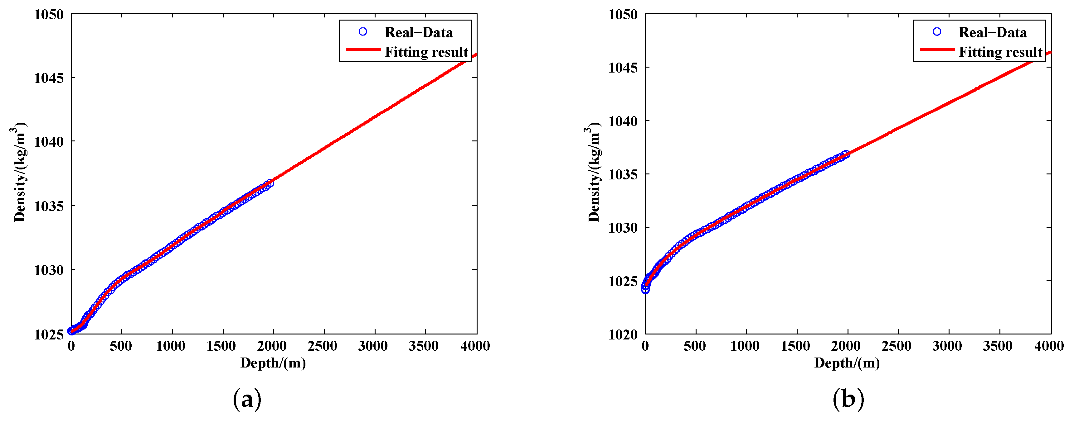
Figure 5.
The fitting result of the density data in the southern hemisphere. Panel (a) shows the seawater’s density data in summer and (b) shows the seawater’s density data in winter.
Figure 5.
The fitting result of the density data in the southern hemisphere. Panel (a) shows the seawater’s density data in summer and (b) shows the seawater’s density data in winter.

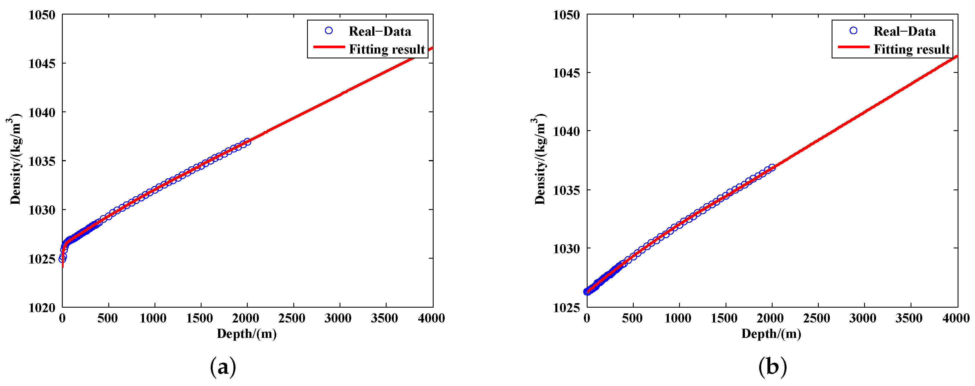
Figure 6.
The fitting result of the density data in the equator area. Panel (a) shows the seawater’s density data in summer and (b) shows the seawater’s density data in winter.
Figure 6.
The fitting result of the density data in the equator area. Panel (a) shows the seawater’s density data in summer and (b) shows the seawater’s density data in winter.

Figure 7.
The fitting result of the density data in the nouthern hemisphere. Panel (a) shows the seawater’s density data in summer and (b) shows the seawater’s density data in winter.
Figure 7.
The fitting result of the density data in the nouthern hemisphere. Panel (a) shows the seawater’s density data in summer and (b) shows the seawater’s density data in winter.

Figure 8.
The fitting effect of the temperature at depth 0 m to 2000 m.

Figure 9.
The fitting result of the temperature data in the southern hemisphere. Panel (a) shows the seawater’s temperature data in summer and (b) shows the seawater’s temperature data in winter.
Figure 9.
The fitting result of the temperature data in the southern hemisphere. Panel (a) shows the seawater’s temperature data in summer and (b) shows the seawater’s temperature data in winter.

Figure 10.
The fitting result of the temperature data in the equator area. Panel (a) shows the seawater’s temperature data in summer and (b) shows the seawater’s temperature data in winter.
Figure 10.
The fitting result of the temperature data in the equator area. Panel (a) shows the seawater’s temperature data in summer and (b) shows the seawater’s temperature data in winter.

Figure 11.
The fitting result of the temperature data in the nouthern hemisphere. Panel (a) shows the seawater’s temperature data in summer and (b) shows the seawater’s temperature data in winter.
Figure 11.
The fitting result of the temperature data in the nouthern hemisphere. Panel (a) shows the seawater’s temperature data in summer and (b) shows the seawater’s temperature data in winter.

Figure 12.
The fitting effect of the oil draining speed and motor’s operating current.

Figure 13.
The one-time oil draining control mode.

Figure 14.
Parameters of the DSPB’s ascent stage of the one-time oil draining method.

Figure 15.
The process of the stage quantitative oil draining control mode.

Figure 16.
The optimization process of the non-dominated sorted genetic algorithm-II (NSGA-II) method.
Figure 16.
The optimization process of the non-dominated sorted genetic algorithm-II (NSGA-II) method.
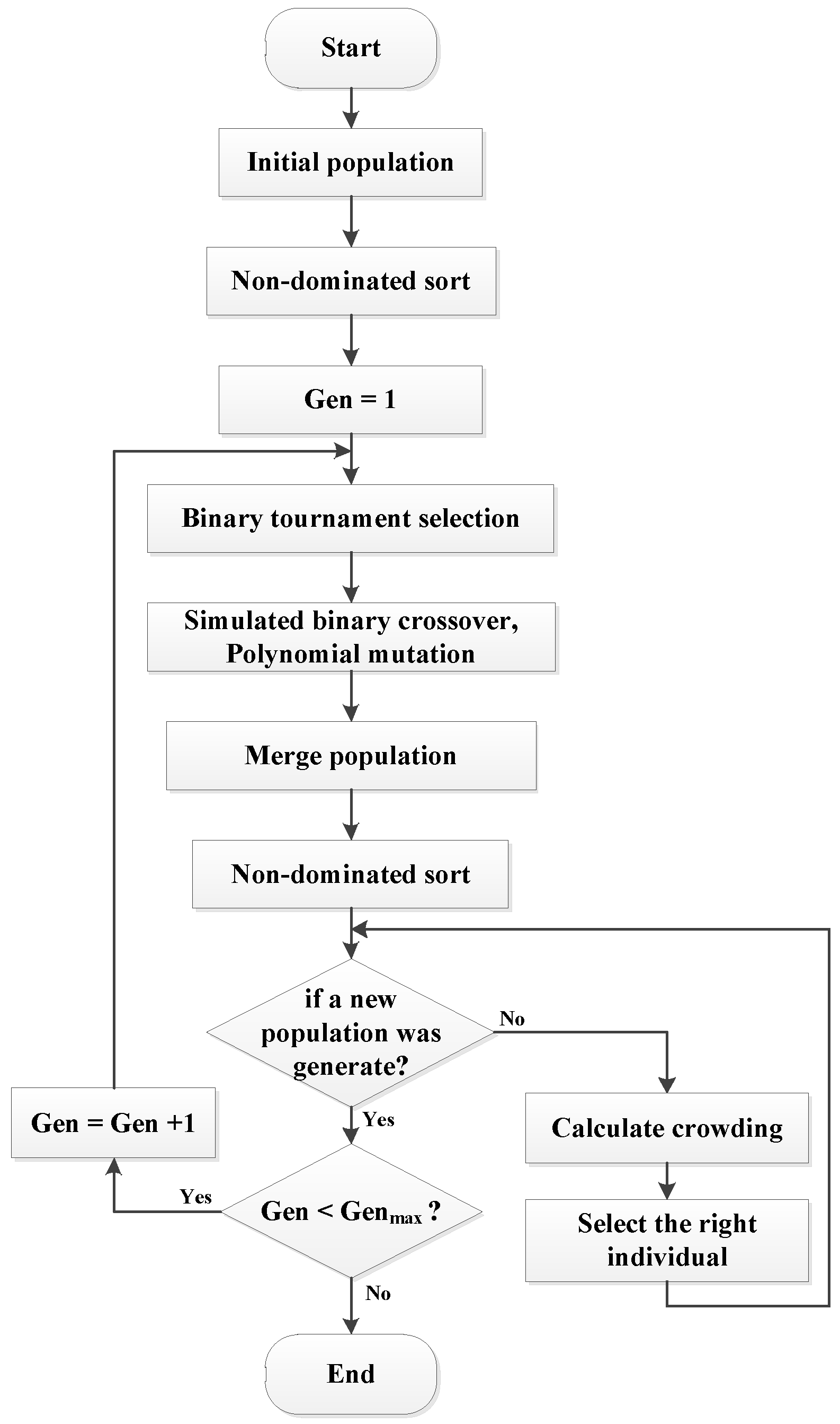
Figure 17.
The optimal result of NSGA-II method with different ODR.

Figure 18.
The optimal result of different optimal parameters. Panel (a) shows the optimal result of different populations and (b) shows the optimal result of different generations.
Figure 18.
The optimal result of different optimal parameters. Panel (a) shows the optimal result of different populations and (b) shows the optimal result of different generations.

Figure 19.
The optimal result of different ODR in the southern hemisphere. Panel (a) shows the optimal result in summer where the total energy consumption reduced by 13.5% and (b) shows the optimal result in winter where the total energy consumption reduced by 12.0%.
Figure 19.
The optimal result of different ODR in the southern hemisphere. Panel (a) shows the optimal result in summer where the total energy consumption reduced by 13.5% and (b) shows the optimal result in winter where the total energy consumption reduced by 12.0%.

Figure 20.
The optimal result of different ODR in the equator area. Panel (a) shows the optimal result in summer where the total energy consumption reduced by 11.9% and (b) shows the optimal result in winter where the total energy consumption reduced by 11.8%.
Figure 20.
The optimal result of different ODR in the equator area. Panel (a) shows the optimal result in summer where the total energy consumption reduced by 11.9% and (b) shows the optimal result in winter where the total energy consumption reduced by 11.8%.

Figure 21.
The optimal result of different ODR in the nouthern hemisphere. Panel (a) shows the optimal result in summer where the total energy consumption reduced by 12.6% and (b) shows the optimal result in winter where the total energy consumption reduced by 10.9%.
Figure 21.
The optimal result of different ODR in the nouthern hemisphere. Panel (a) shows the optimal result in summer where the total energy consumption reduced by 12.6% and (b) shows the optimal result in winter where the total energy consumption reduced by 10.9%.

Figure 22.
The optimal result of traversal method (ODR = 50 mL).

Figure 23.
Optimal results of multi-objective optimization model. Panel (a) shows the Pareto optimization results and (b) shows the variety of the hypervolume value.
Figure 23.
Optimal results of multi-objective optimization model. Panel (a) shows the Pareto optimization results and (b) shows the variety of the hypervolume value.

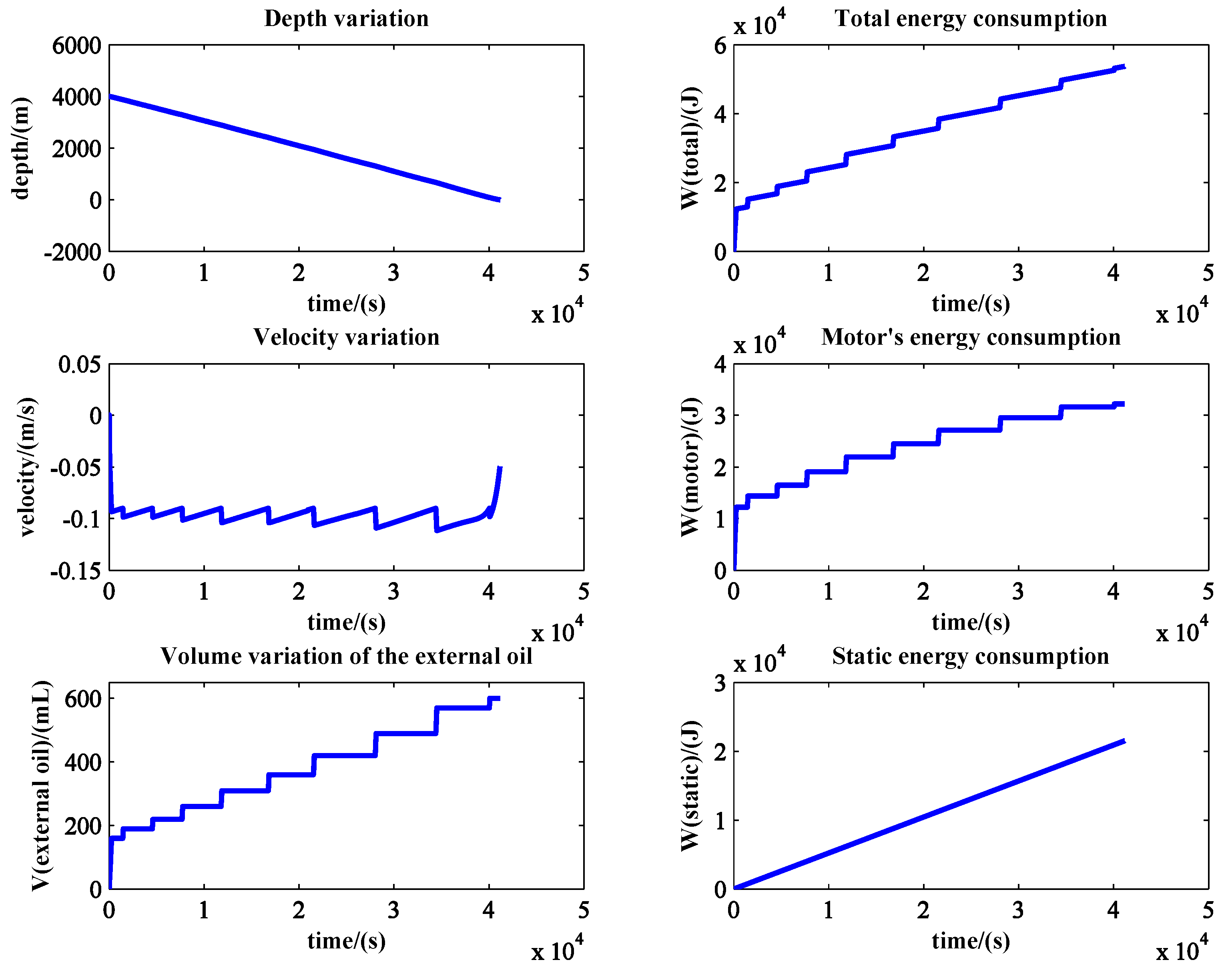
Figure 24.
Parameters of the DSPB’s ascent stage optimized by the NSGA-II method.


Table 1.
The running states of devices and sensors of the deep-sea self-sustaining profile buoy (DSPB) in the whole working stage.
Table 1.
The running states of devices and sensors of the deep-sea self-sustaining profile buoy (DSPB) in the whole working stage.
| Devices and Seneors | First Descent | Hovering | Second Descent | Ascent | Surface Communication |
|---|---|---|---|---|---|
| CTD sensor | ● | ● | ● | ● | ● |
| Steering engine | ◖ | ◖ | ◖ | ○ | ○ |
| Oil pump motor | ○ | ◖ | ○ | ◖ | ○ |
| GPS module | ○ | ○ | ○ | ○ | ● |
| Comet module | ○ | ○ | ○ | ○ | ● |
| Embedded control system | ● | ☉ | ● | ● | ● |
● Running, ○ not running, ◖ running if necessary, ☉ Standby mode.
Table 2.
The coefficient values for polynomial fitting of .
Table 3.
The coefficient values for polynomial fitting of .
Table 4.
The coefficient values for polynomial fitting of .
Table 5.
The coefficient values for polynomial fitting of .
Table 6.
The coefficient values for polynomial fitting of .
Table 7.
The coefficient values for polynomial fitting of .
Table 8.
The coefficient values for polynomial fitting of .
Table 9.
Parameters of proposed non-dominated sorted genetic algorithm-II (NSGA-II) method.
| Size of population | 50 |
| Chromosome structure | Real number coding |
| Selection scheme | Binary tournament selection |
| Reproduction | Simulated binary crossover and Polynomial mutation |
| Produced distribution index | 20 |
| Selected distribution index | 20 |
| Maximum generation | 200 |
Table 10.
Optimization time of different optimal parameters.
| Parameters of NSGA-II | Optimization Time (s) |
|---|---|
| population = 50, generation = 100 | 3487.088273 |
| population = 25, generation = 200 | 3609.206185 |
| population = 50, generation = 200 | 7315.951831 |
| population = 75, generation = 200 | 10,455.033943 |
| population = 50, generation = 300 | 10,513.551947 |
| population = 100, generation = 200 | 13,965.117581 |
Table 11.
The optimization effect of the NSGA-II method after 10 repetitions.
| Execution Times | Optimal (J) | Optimal ( m/s) | Optimal ( mL) | Optimization Time(s) |
|---|---|---|---|---|
| 1 | 53,731.76245 | 0.09 | [180,50,50,60,70, | 7227.545857 |
| 70,90,20,10] | ||||
| 2 | 53,720.31747 | 0.09 | [170,30,40,40,60, | 7191.563176 |
| 50,50,70,90] | ||||
| 3 | 53,731.76245 | 0.09 | [180,50,50,60,70, | 7404.939277 |
| 70,90,20,20] | ||||
| 4 | 53,716.03741 | 0.09 | [170,30,40,30,40, | 7047.592007 |
| 50,60,70,90,20] | ||||
| 5 | 53,727.2845 | 0.09 | [180,40,10,50,60, | 7015.543344 |
| 60,60,60,80] | ||||
| 6 | 53,718.10196 | 0.09 | [170,30,20,40,40, | 7163.158171 |
| 60,60,70,80,30] | ||||
| 7 | 53,722.04461 | 0.09 | [160,40,40,40,30, | 7404.939277 |
| 40,60,70,90,30] | ||||
| 8 | 53,716.84258 | 0.09 | [160,30,30,40,50, | 7047.592007 |
| 50,60,70,80,30] | ||||
| 9 | 53,717.98512 | 0.09 | [160,30,30,40,50, | 7015.543344 |
| 60,60,70,80,20] | ||||
| 10 | 53,720.96775 | 0.09 | [180,40,40,40,50, | 7163.158171 |
| 60,70,80,40] |
Table 12.
Parameters of proposed NSGA–II algorithm for multi-objective optimization.
| Size of Population | 50 |
| Chromosome Structure | Real number coding |
| Selection Scheme | Binary tournament selection |
| Reproduction | Simulated binary crossover and Polynomial mutation |
| Produced Distribution Index | 20 |
| Selected Distribution Index | 20 |
| Maximum Generation | 600 |
Table 13.
The optimization effect of the NSGA-II method compared with pre-optimization.
| Before Optimization | After Optimization | Optimal Ratio | |
|---|---|---|---|
| (mL) | [600] | [160,30,30,40,50,50,60,70,80,30] | – |
| (m/s) | – | 0.9 | – |
| t (s) | 28,704 | 40,699 | – |
| (J) | 15,007.51 | 21,278.95 | – |
| (J) | 45,325.47 | 32,198.96 | 28.9% |
| (J) | 60,332.98 | 53,716.84 | 11.0% |
© 2019 by the authors. Licensee MDPI, Basel, Switzerland. This article is an open access article distributed under the terms and conditions of the Creative Commons Attribution (CC BY) license (http://creativecommons.org/licenses/by/4.0/).
Share and Cite
MDPI and ACS Style
Liu, M.; Yang, S.; Li, H.; Xu, J.; Li, X. Energy Consumption Analysis and Optimization of the Deep-Sea Self-Sustaining Profile Buoy. Energies 2019, 12, 2316. https://doi.org/10.3390/en12122316
AMA Style
Liu M, Yang S, Li H, Xu J, Li X. Energy Consumption Analysis and Optimization of the Deep-Sea Self-Sustaining Profile Buoy. Energies. 2019; 12(12):2316. https://doi.org/10.3390/en12122316
Chicago/Turabian StyleLiu, Mingcong, Shaobo Yang, Hongyu Li, Jiayi Xu, and Xingfei Li. 2019. "Energy Consumption Analysis and Optimization of the Deep-Sea Self-Sustaining Profile Buoy" Energies 12, no. 12: 2316. https://doi.org/10.3390/en12122316
Note that from the first issue of 2016, this journal uses article numbers instead of page numbers. See further details here.