2.1. Selecting the Model of STLF
Many models are currently used for STLF in Vietnam. However, the three main models are:
Model 1: Combining peak and valley load and daily load pattern.
Model 2: Directly forecasting 24 h daily load at the same time.
Model 3: Forecasting instantaneous power load step by step of 1 h.
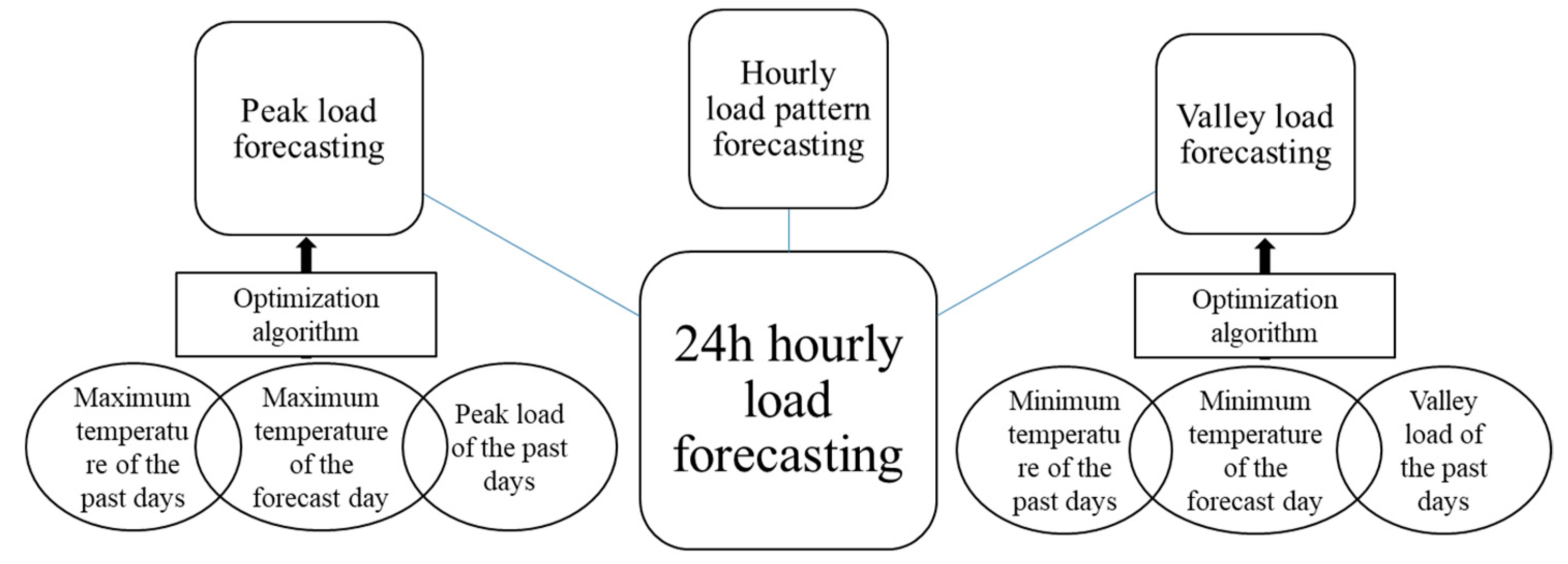
This work selects the Model 1 illustrated in [
18]. This model consists of three separate parts: the maximum real load power (peak load) forecasting, the minimum real load power (valley load) forecasting and the identified day types (load pattern). The overview of this model is demonstrated in
Figure 1.
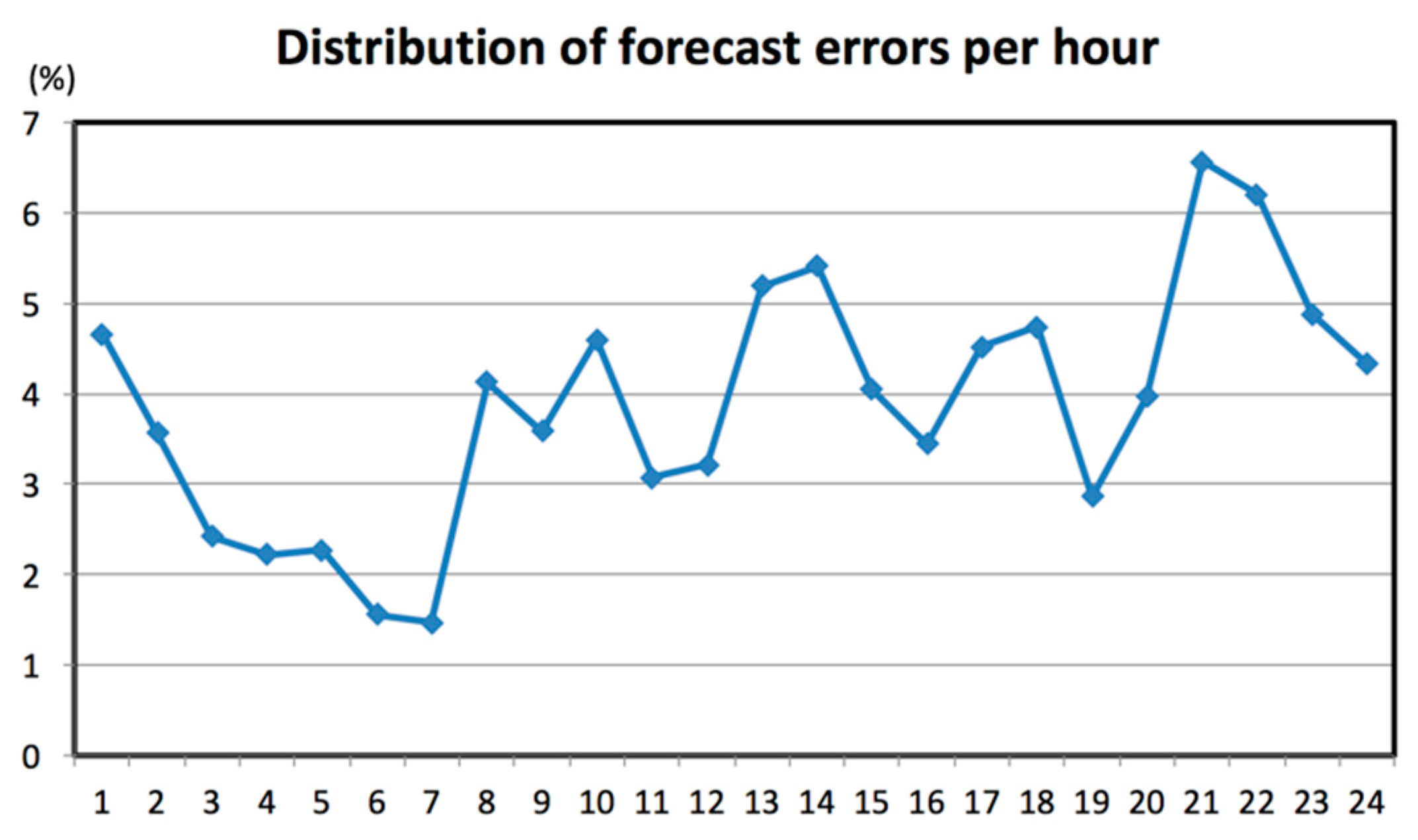
In this model, the forecast error depends on all three parts: peak and valley load and load pattern forecasting. The peak and valley load errors are usually smaller than the load pattern. The partial errors in this model are differentiated and optimized separately to gain suitable adjustments during the grid operation for minimizing the errors in future forecasting.
2.3. Determining the Load Pattern
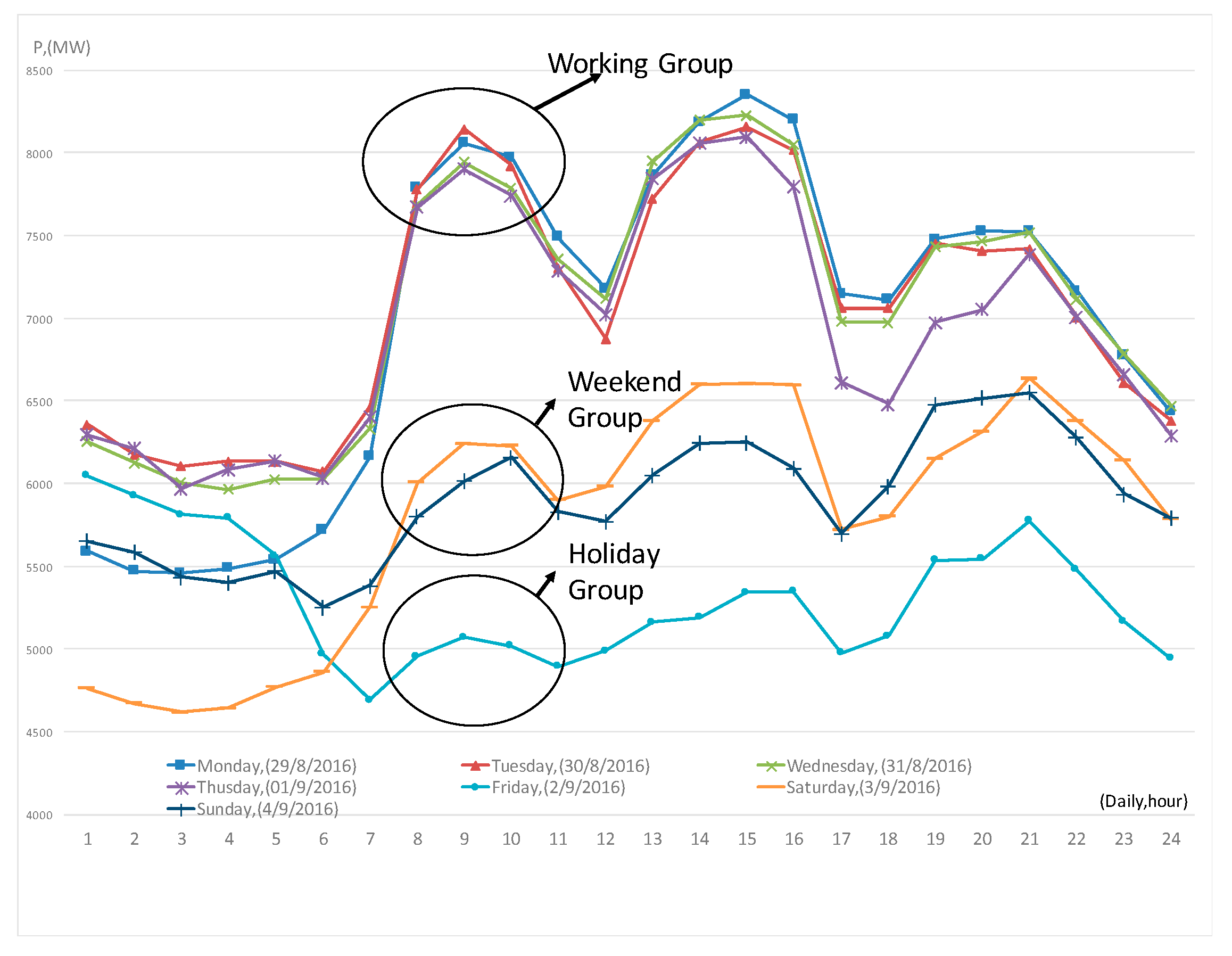
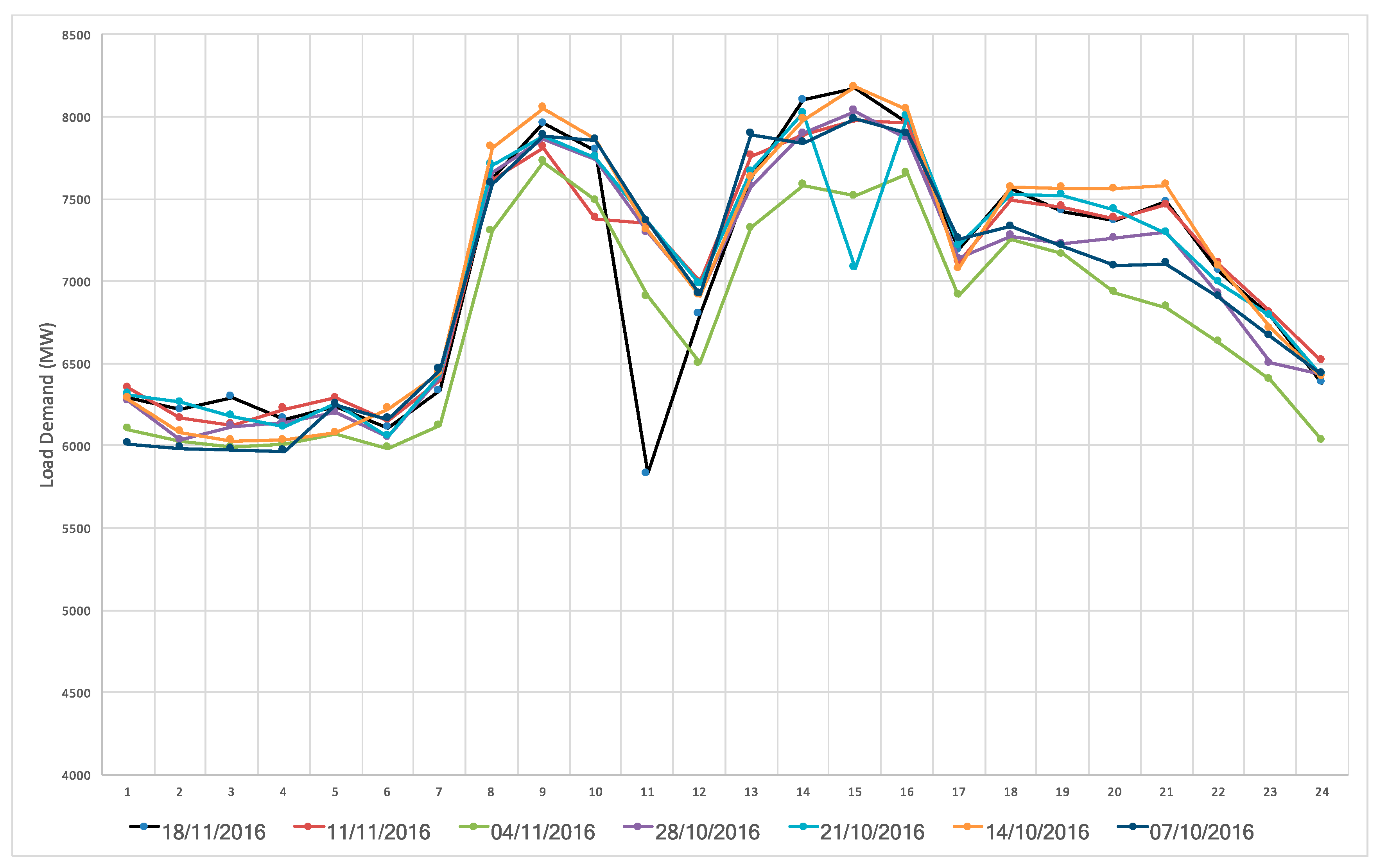
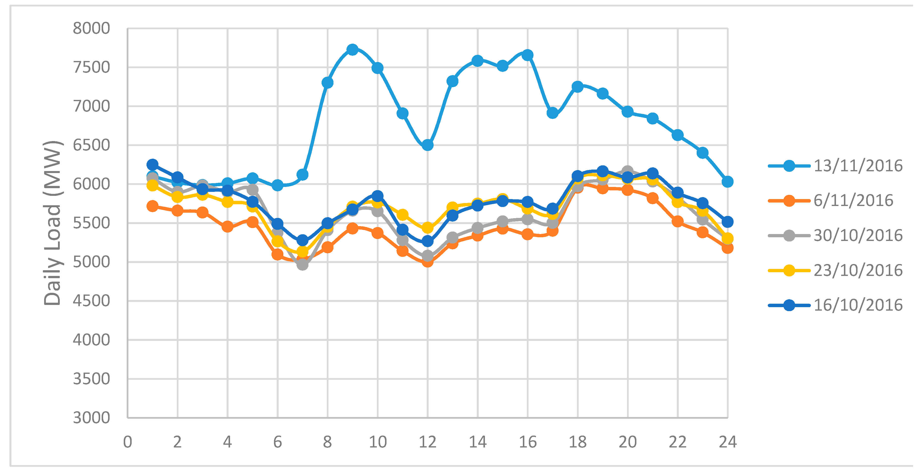
Calculating the load pattern greatly affects the accuracy of the forecasting. There are several published forecast methods but the most effective method is still based on the experience of predictors to choose previous days with similar load patterns as the forecast day. In our method, all days may be classified in terms of the daily load pattern into eight groups: five working day groups (from Monday to Friday), two weekend groups (Saturday and Sunday), and one holiday (or special-event day) group. The demonstration of load’s characteristics can be observed in the case of one week in
Figure 2 (from 29 August to 3 September 2016). This week consists of a holiday (Friday, 2 September, is Vietnam Nation day). The differences among the three groups is striking: working days, weekend and holidays. However, caused by characteristics of SPC’s load, each day of the week has its own load pattern, which is further distinguished if it coincides with a holiday.
In this article, five similar days (holiday, day of week, and season of year) are used to reform Equation (1). Then, the normalized load pattern is calculated by the average formula:
where
Pij is the normalized hourly load of the selected similar days. During the normalization, we eliminate some days if there are sudden differences on the load pattern graph by checking the correlative coefficients with two steps:
- -
Calculate the correlative coefficients between the similar days by the CORREL function.
- -
Evaluate the value of correlative coefficients and eliminate the days corresponding to the value out of range [0.9, 1].
2.4. Selecting the GA Algorithm
Currently, Genetic Algorithm (GA) is one of the most popular algorithms on research using ANN. The basic knowledge of GA is described clearly in Vietnamese and international publications. Therefore, we do not focus on describing GA in this paper but only using GA to apply the load forecasting for a Vietnamese power company.
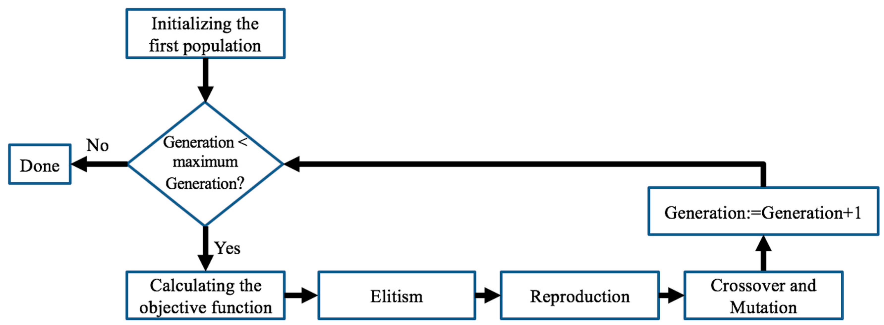
GA has shown to be a strong and fairly accurate algorithm in research about optimization problems for a large power system. There are many GA-based studies in the field of STLF. In 1994, Maifeld et al. [
19] published STLF research based on ANN and GA. In this article, the authors called the basic GA by the name of RGA. RGA also includes three operators: reproduction, crossover and mutation. The diagram of RGA is shown in
Figure 3; however, the order of steps is different from other studies.
Maifeld et al. [
19] provided comparisons between back propagation (BP) and RGA on forecasting of 12 h of a day. The errors are shown in
Table 1.
Although the error of RGA is smaller than the one of BP algorithm, the authors stated that the execution time of RGA is much greater.
Several studies focus on optimizing the ANN operations instead of improving GA. One successful approach was presented by Ling et al. [
20]. They compared results using the traditional ANN and an improved ANN integrating the same GA. The object of this publication is the household daily load. On that, the GA affects only some hidden class neurons to create a well-trained neural network with respect to the fitness value. Recently, studies on ANN using GA are mostly improved using hybrid algorithms, where GA acts as one of the main partners. The hybrid algorithm usually exploits basic GA with three key operators: reproduction, crossover and mutation. In each operator, it is absolutely necessary to select key parameters. In [
21,
22], the encryption is of two kinds, namely encryption by binary string and encryption by real value; the crossover consists of three types, namely the crossover-weights, the crossover-nodes and the crossover-features; and the mutation can be either unbiased or biased. Finally, the key parameters were determined as below:
- -
Crossover method: Crossover-weights
- -
Mutation method: Biased (with fixed probability 0.1)
2.5. Selecting the PSO Algorithm
2.5.1. Overview of PSO Algorithms
The construction of PSO was first articulated by J. Kennedy and R.C. Eberhart (1995) [
23] and improved step-by-step in their later publications. The basic PSO is defined as:
where
is the velocity of particle i at the loop k;
is the position of particle i at the loop k;
and are the learning fixed factors;
and are random values within (0,1);
is the best position of particle i at the loop k; and
is the best position of swarm at the loop k.
Note that choosing > shows the bias direction of the swarm’s movement according to individual optimization (Pbest) or global optimization (Gbest) and thus affects the convergence rate of PSO.
To avoid the separation of the swarm caused by the speed of movement, a proposed speed limit is set at each iteration [
24]. However, the speed limit also adversely affects to the swarm’s searching space. By this conflict, a parameter
w (a constant or even a function) called the “inertia weight” was given by Y. Shi and R.C. Eberhart [
25]. The inertia weight si brought into the basic PSO as shown in Equation (5) (an advanced PSO):
The authors of [
26,
27] utilized Equation (6) to give the inertia weight
wk on each iteration of swarm:
where
k stands for the actual number of epochs and
kmax is the maximum number of epochs.
The authors showed that the recommended range for [wmin, wmax] is [0.4, 0.9].
The participation of inertia weights w aims to avoid the swarm’s separation; however, the algorithm may still fall into the local convergence in the case of the multidimensional searching space. This is caused by information exchange mechanism among particles in the swarm. Thus, another modified PSO was proposed for this mechanism. Instead of exchanging information with all particles in the swarm, each one exchanges information of position and velocity in a group of similar particles. Therefore,
Gk in the basic PSO is replaced by
Lk, meaning the optimal local value. The general equations of this advanced PSO is as follows:
One of the new PSO trends is Stand PSO (SPSO), which is currently presented in many studies on PSO applications. The first was conducted by Ozcan and Mohan [
28]. Their results show the movement of particles in the searching space. A few years later, their research was updated with more details by Clerc and Kennedy [
29], who analyzed the convergence of the algorithm. The SPSO is defined as:
This model may also be applied to the advanced PSO mentioned in Equation (7):
where
X is called by the constriction factor. This research experimentally demonstrated the optimal value of
X by the following formula:
As mentioned above, SPSO focuses primarily on the convergence of the algorithm. The selected coefficients also aim to accelerate the convergence speed while ensuring the accuracy of the optimization. However, as we know, rapid convergence also means the possibility of falling into local convergence traps. Therefore, we need to choose either PSO or SPSO to combine with GA in our hybrid algorithm before applying to a specific subject. To select which PSO to combine with the hybrid algorithm, we separately implemented both modified PSO algorithms (basic PSO and SPSO). After that, the load forecasting was compared using the predictive errors. In addition, the rate of convergence was also considered by comparing the graphs of the value of objective function (MSE-mean square error) according to each iteration. Due to the data source collection, we utilized the available dataset of Southern Power Corporation (SPC:
https://evnspc.vn/) in 2014.
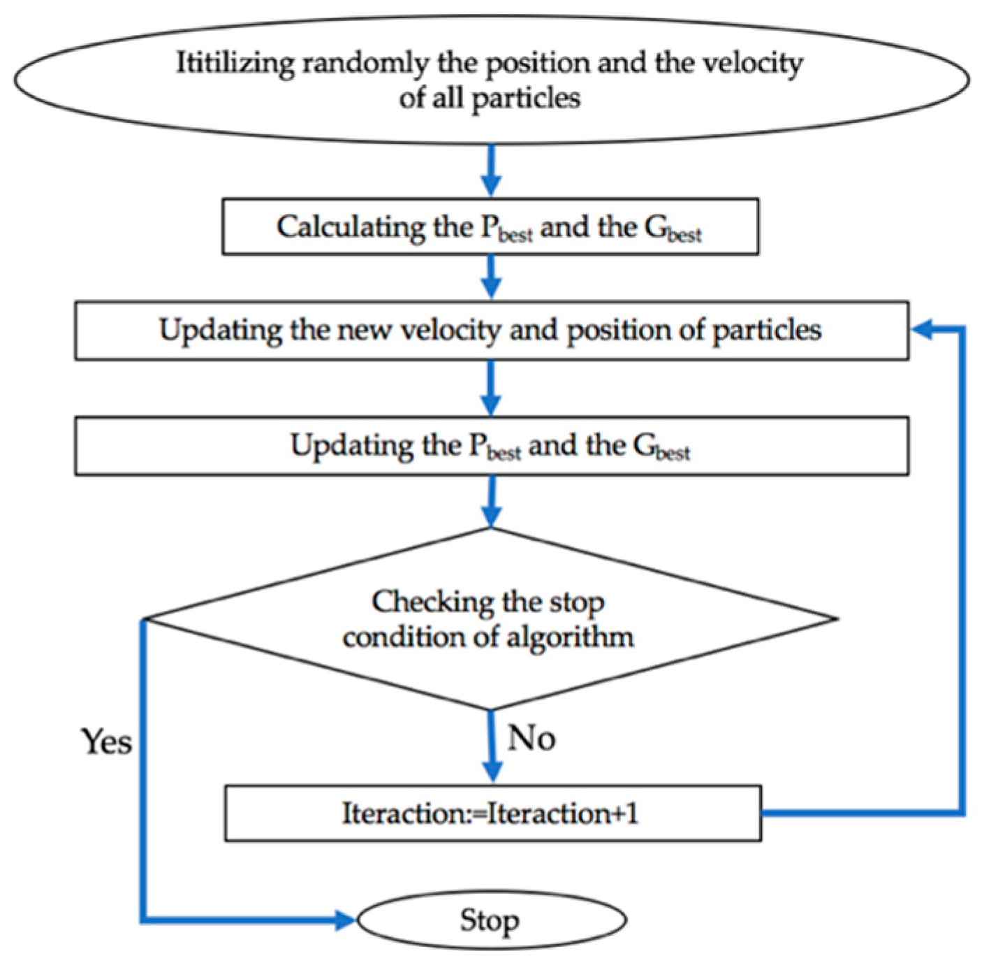
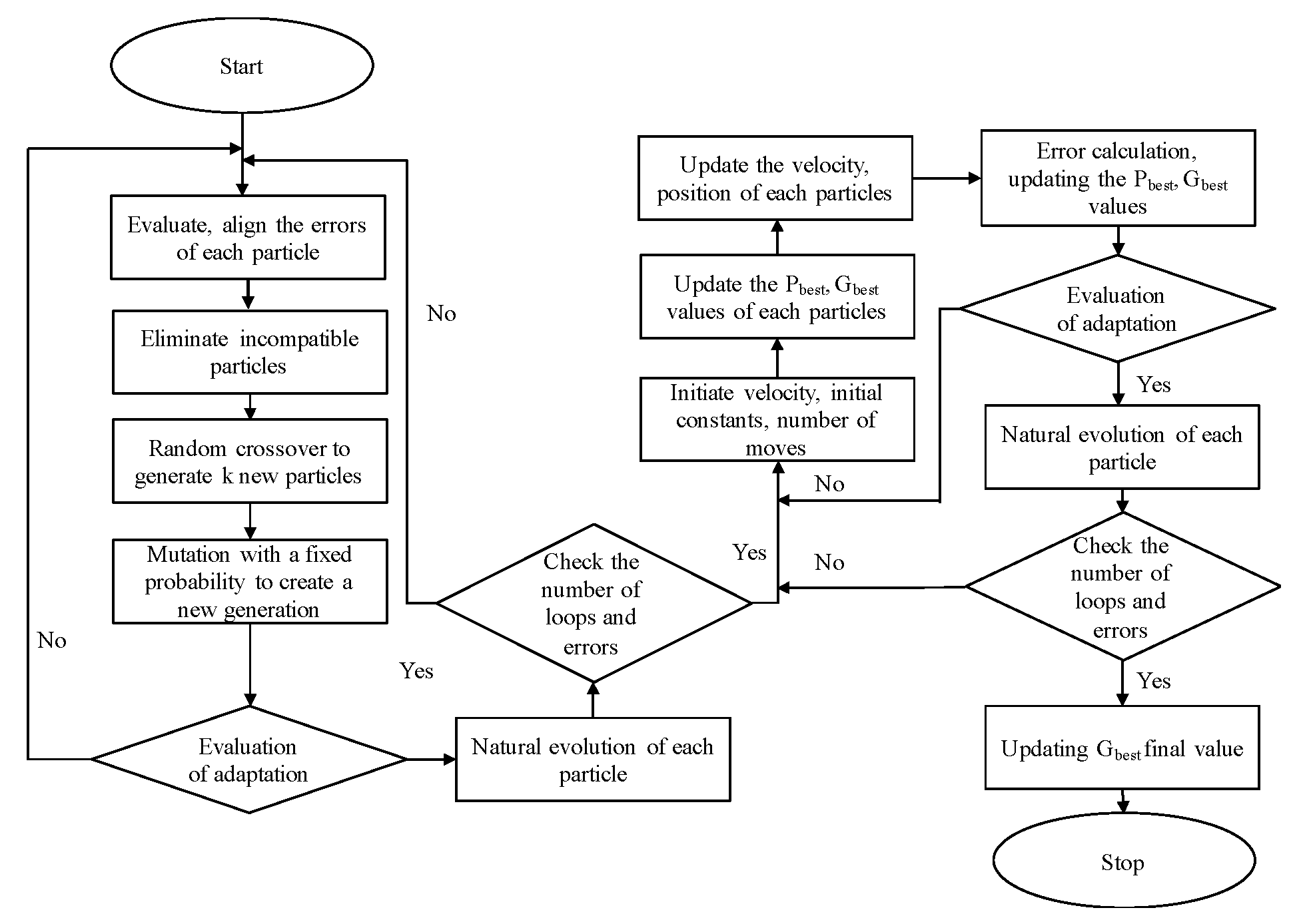
2.5.2. Comparison between PSO and SPSO
Both PSO algorithms were tested with the same algorithm shown in
Figure 4.
The PSO algorithms were configured with the following coefficients:
The Basic PSO:C1 = 2 and C2 = 1. The values of C1 and C2 represent the movement priority of particles according to Pbest or Gbest. The value of C1 being more than C2 denotes the reduction of rate of signal propagation to Gbest of the swarm. This also helps overcome the disadvantage relating to the local convergence traps. R1 and R2 are random coefficients in the range of [0,1]. According to the above-mentioned studies, the value of w decreases from wmax = 0.9 to wmin = 0.4. However, during the simulating process, the decrease of w on the next iterations would reduce the movement speed of the swarm, leading to fall into the local convergence traps. Thus, we propose a solution to overcome this disadvantage. In the first 100 iterations, the value of w decreases from 0.9 to 0.4 according to Equation (6). From Iteration 101, the value of w remains equal to 0.9. This solution will help the swarm searching space be big enough to increase the likelihood of finding the optimal solution.
The SPSO: According to Clerc and Kennedy [
29], the value of coefficients significantly affects the error of an algorithm. By empirical simulations, the optimal values of coefficients were relatively determined as follows:
X = 0.729;
C1 = 2.05;
C2 = 2.05; and
R1 and
R2 randomly fixed in the range of [0,1].
Table 2 shows the comparison between the basic PSO and the SPSO.
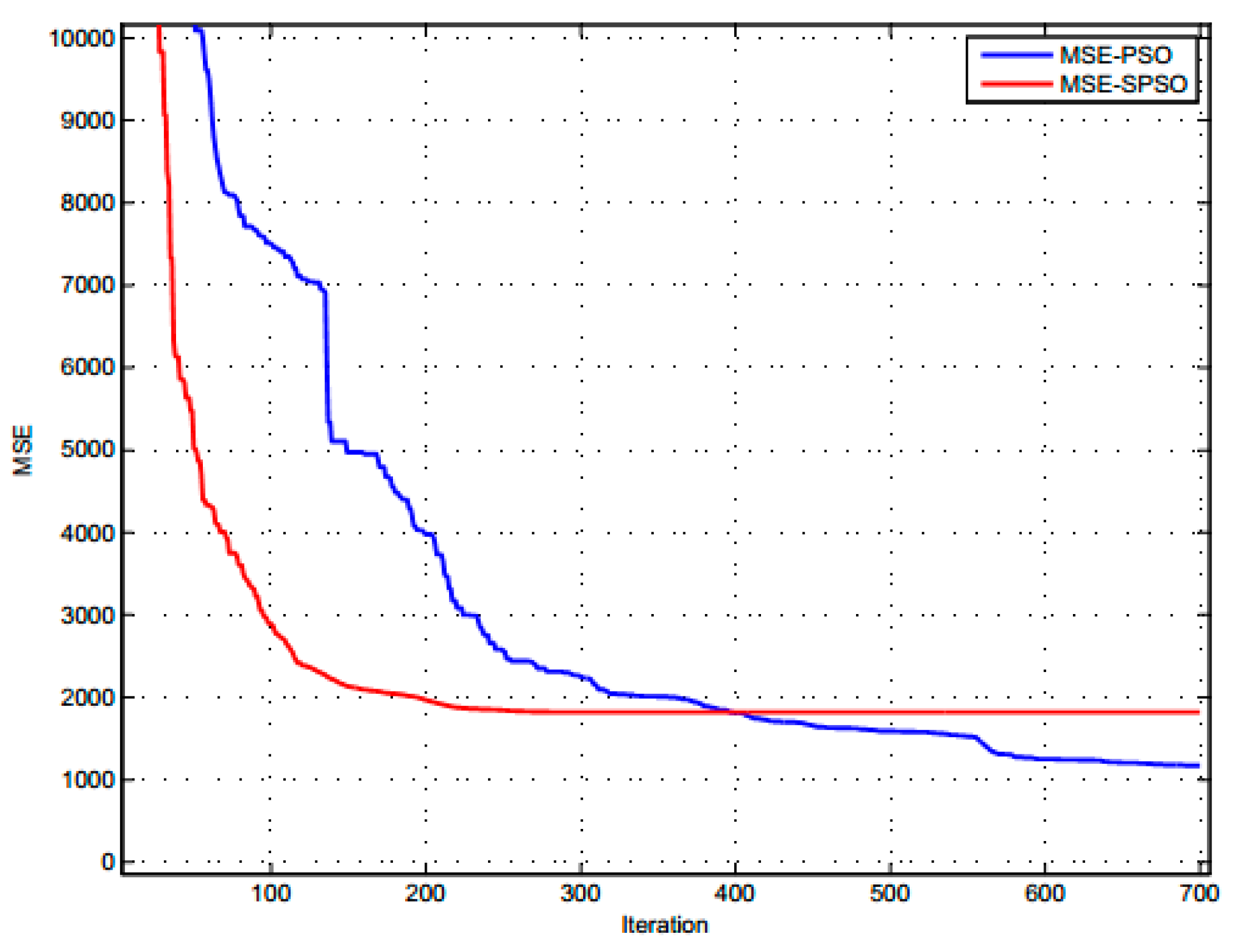
The basic PSO is slightly better than SPSO but the difference is still not clear. To be able to see more clearly the process of both algorithm, the MSE value of each training process was analyzed and represented as a graph.
Figure 5 shows the MSE value through each iteration.
MSE value with SPSO reduces very quickly during the first 100–200 iterations. Then, it almost does not change. This is the main disadvantage of SPSO algorithm because SPSO is researched and developed to increase the convergence speed of the swarm. We can see that, if the number of iterations is bigger, the value of MSE almost insignificantly decreases. Thus, the accuracy of the algorithm is not improved with more interations.
MSE value with basic PSO has a slower reduction than SPSO but, after 200 iterations, the MSE value continues to decrease steadily and is smaller than SPSO’s from about 400 iterations. This shows the positive effect of adjusting the value of inertia weight w after 100 iterations (remaining equal to 0.9).
By comparing the two PSO algorithms, we conclude that applying SPSO algorithm to load forecasting only increases the speed of implementation but does not improve the result and it may fall into the local convergence traps. Meanwhile, we can still improve the error of result by increasing the number of iterations with the basic PSO. Therefore, we chose the basic PSO to combine with GA in the GA-PSO hybrid algorithm applied in the load forecasting of SPC.
2.6. Selecting the Hybrid GA-PSO Algorithm
As we known, an optimal algorithm also may apply to all studies of optimization. H. Garg [
14] conducted research using the GA-PSO hybrid algorithm to solve a nonlinear optimization problem. The roles of GA and PSO are clearly described in
Figure 6.
In this combination method, the GA is used to optimize each individual in the swarm. Accordingly, the GA algorithm must be executed continuously with both crossover and mutation operators. This greatly increases the runtime of the simulation.
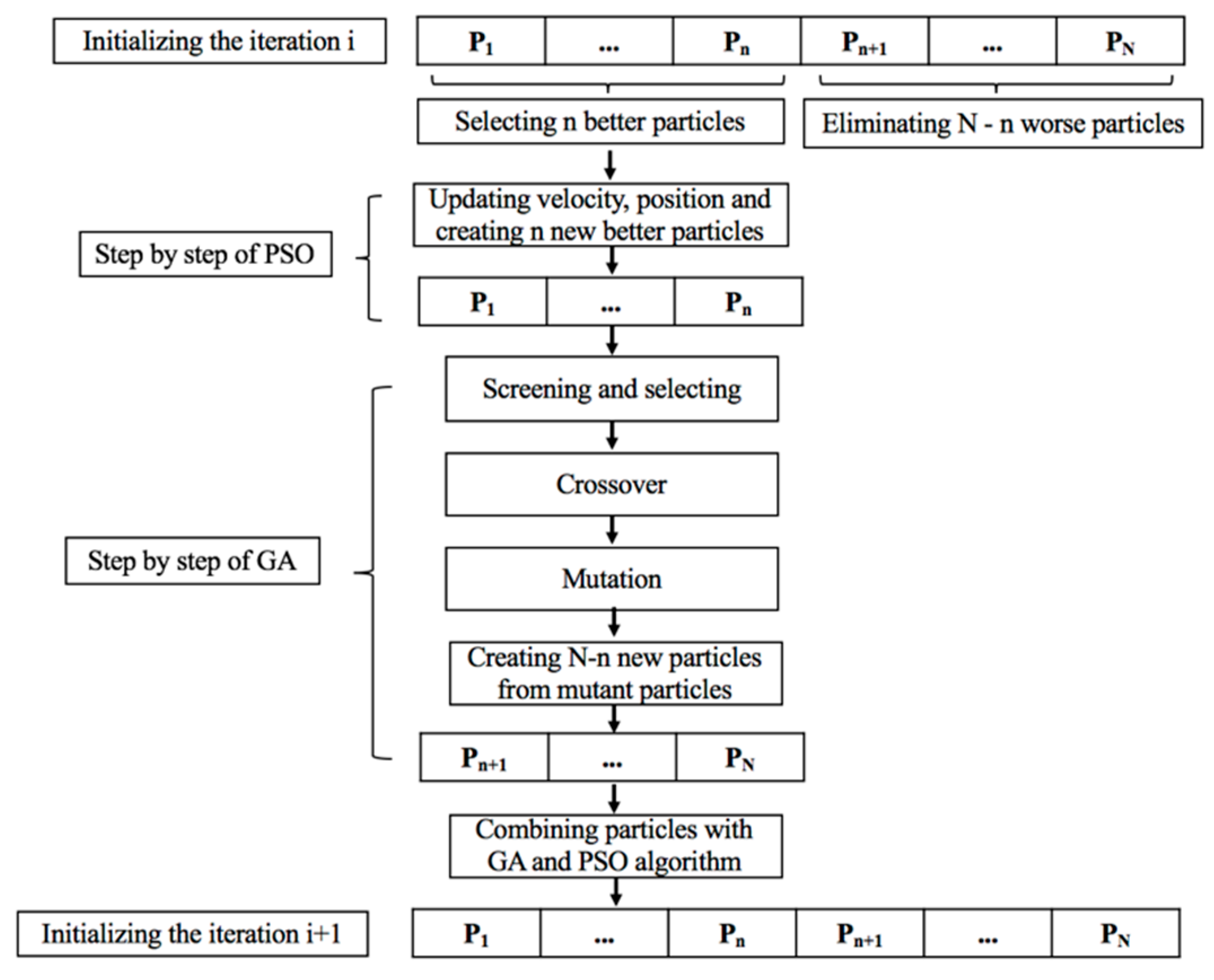
Using the same idea as Harish Garg (PSO algorithm is used to select better individuals of the initial iteration before performing steps of evolution), Q. Zhang et al. [
15] provided a simpler algorithm to optimize the parameters of direct-injection diesel engine running with soy biodiesel. The PSO algorithm is done on the
n best individuals, thus producing n offspring for use in the next iteration (generation). The remaining
N-n individuals are eliminated to make room for the new better individuals generated by GA step. This step aims to create a new generation with the same quantity of particles of swarm. The flowchart of this combination method is presented in
Figure 7.
Following this research, the authors mentioned the optimal runtime of hybrid PSO-GA algorithm in comparison to basic GA and basic PSO. However, demonstrating the comparison between PSO-GA and single PSO is not shown. In another study using a parallel combination of GA-PSO, Sahoo et al. [
16] also presented similar comparisons and mentioned the inherent weakness of runtime if GA algorithm executes iterations in more than one program loop. Therefore, in our hybrid algorithm, GA algorithm is implemented first and does not repeat in any other loop to avoid this drawback. After that, PSO loops perform its optimal work. This is a helpful, simple solution to apply to load forecasting in Vietnam. The GA step is implemented independently of PSO.
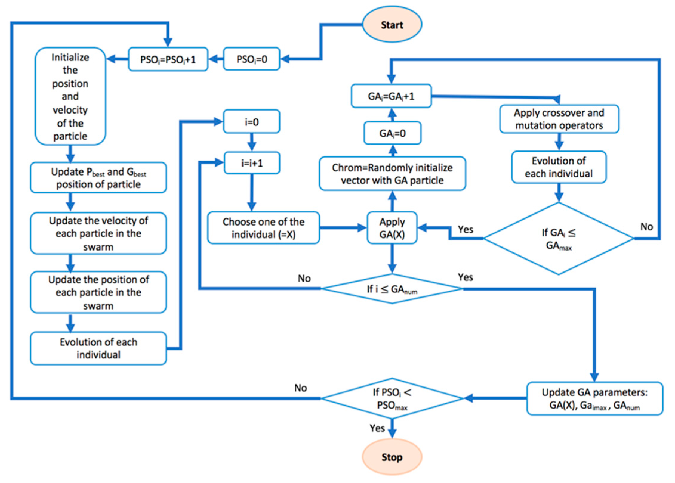
2.6.1. Step by Step of the Selected Hybrid Algorithm
The steps of combining GA and PSO algorithms in the progress of optimizing the ANN’s parameters for application to load forecasting are briefly described according to
Figure 8. All detailed steps are listed in order below.
Genetic Algorithm
Step 1: Prepare the data for ANN.
Step 2: Configure the ANN.
Step 3: Initialize the first weights (particle in swarm) and the number of generations.
Step 4: Train ANN with each generated particle using the same load data. Calculate the respective errors (MSE values).
Step 5: After obtaining the MSE values, sort them in ascending order and then remove the large value errors from the swarm (natural selection).
Step 6: With the remaining particles of the swarm, randomly implement the crossover together to generate the new particles, ensuring the initial population size remains unchanged.
Step 7: Implement the mutation step with selected probability.
Step 8: Assess the adaptability of new generation with MSE error and stop the loop.
Step 9: Implement natural evolution until one of the stop requirements is attained.
Particle Swarm Optimization
Step 10: Initialize the velocity, the position, the constants and the number of iterations. Take the first generation of swarm from the GA loop.
Step 11: Integrate particles on ANN and simulate to pick of the MSE errors. Calculate the Pbest of each particle and Gbest of the swarm.
Step 12: Calculate the velocity of each particle and update for all.
Step 13: Train the ANN with the new generation of the swarm. Calculate and save the MSE errors. End the iteration.
Step 14: Continue the swarm’s natural evolution until the maximum iteration.
Step 15: Take the final Gbest to train the ANN for load forecasting.
This hybrid algorithm is implanted in the ANN structure as demonstrated:
- -
Structure type: feedforward network
- -
Neuron quantity of input layer: 13
- -
Neuron quantity of output layer: 1
- -
Quantity of hidden layers: 1
- -
Neuron quantity of hidden layer: 5
- -
Fitness function in GA-PSO: MSE
2.6.2. GA-PSO vs. Basic PSO
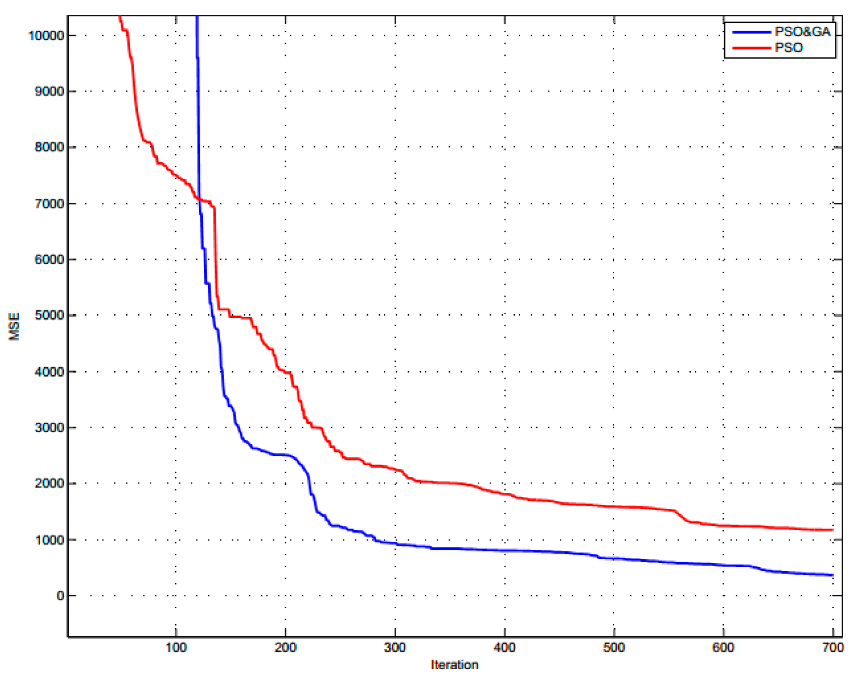
Usually the accuracy of load forecasting using the GA-PSO hybrid algorithm would be demonstrated by comparison with basic GA and basic PSO. However, in discussing the results from simulation, we decided not to compare with simulation using basic GA due to its big errors. Therefore, in this section, we only show simulation results using GA-PSO hybrid algorithm and the basic PSO algorithm. To ensure the total of iterations corresponding to the simulation using basic PSO (700 iterations), we performed 100 iterations with GA and 600 iterations with PSO algorithm. This is an imperfect comparison because one iteration of GA is not the same as one of PSO. However, we could compare the two simulation results. The comparison of MSE errors according to each iteration between these two algorithms is demonstrated by
Figure 9.
It is easy to see that, in the first iterations, the MSE value with GA decreased more slowly than the PSO algorithm, but, after that, the MSE value dropped very quickly and gradually surpassed the one using the basic PSO algorithm. Meanwhile, after 100 iterations, the MSE value using the basic PSO algorithm began to decrease more slowly. This shows that GA algorithm make the MSE value to achieve relatively good accuracy to continue the evolution with PSO algorithm, ensuring the large search space of the swarm.
There are two issues to keep in mind when using hybrid GA-PSO algorithm:
Accuracy of GA algorithm decreased more slowly than PSO algorithm. Therefore, if the total of iterations with GA were too large, it would reduce the overall performance of hybrid algorithm.
One of the operators in GA algorithm is crossover, meaning that more iterations being implemented will lead to more individuals of future generations having more characteristics of their parent individuals, thus they will gradually become more similar. Thus, if the total iterations with GA were too large, the initial weights would be nearly the same or, in other words, the search space of the swarm would be smaller. This would lead to the reduction of performance of the hybrid algorithm. Accordingly, we infer that the selected total iterations with GA needs to be balanced (depending much on the experience of the forecaster) to bring the most efficiency to the whole ANN training process.


