Data-Driven Mitigation of Energy Scheduling Inaccuracy in Renewable-Penetrated Grids: Summerside Electric Use Case


Abstract
:1. Introduction
- Leveraging a relatively large island grid’s actual data to reveal the potential of state-of-the-art time series prediction techniques, in particular for wind energy. Note that, due to commercial IP confidentiality, the details of the prediction engine cannot be revealed; however, general procedures for enhancing RES prediction accuracy is discussed using actual data.
- Proposing a data-driven approach toward BESS sizing for energy balancing purposes. Using actual data, a novel probabilistic approach is proposed that accounts for intra-interval variations, thus enhancing the accuracy of BESS sizing. In general, the proposed method mitigates the trade-off between time resolution and accuracy; as a result, increasing the computation time-interval would have a less significant negative impact on accuracy of the results. Hence, such a method would also alleviate computational burden of analytical methods for BESS sizing. To the knowledge of the author, this is the first time such an approach is proposed in the literature.
- Proposing an optimal BESS energy management based on the presented data-driven approach.
- Quantitative analysis of wind-BESS impact on energy cost using a large amount of actual data.
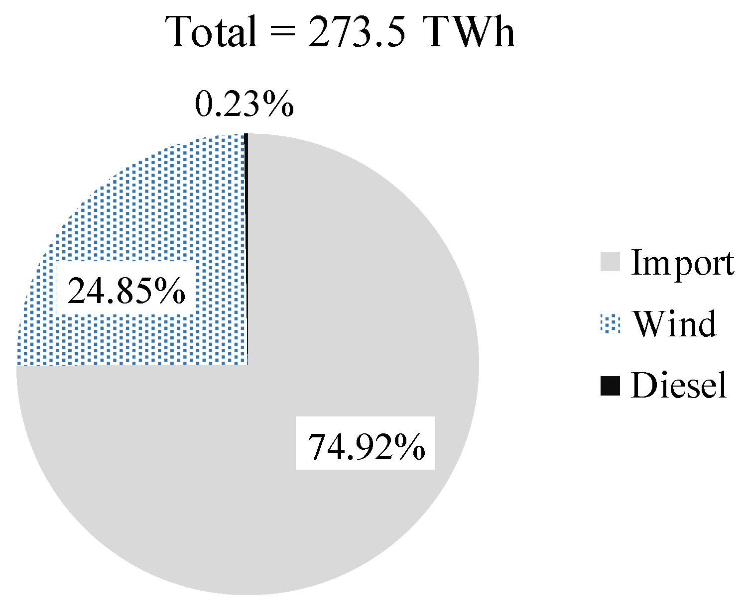
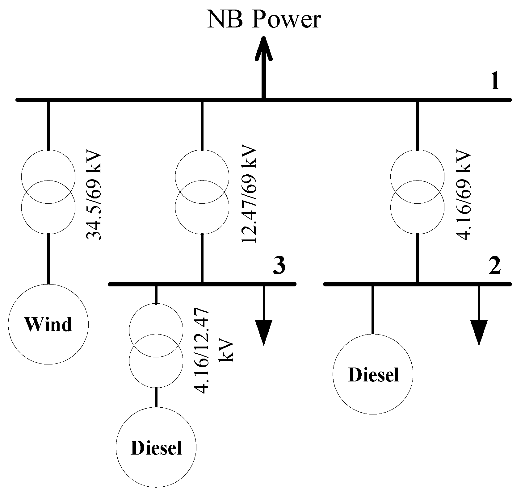
2. Summerside Electric Grid
3. Wind Power Prediction
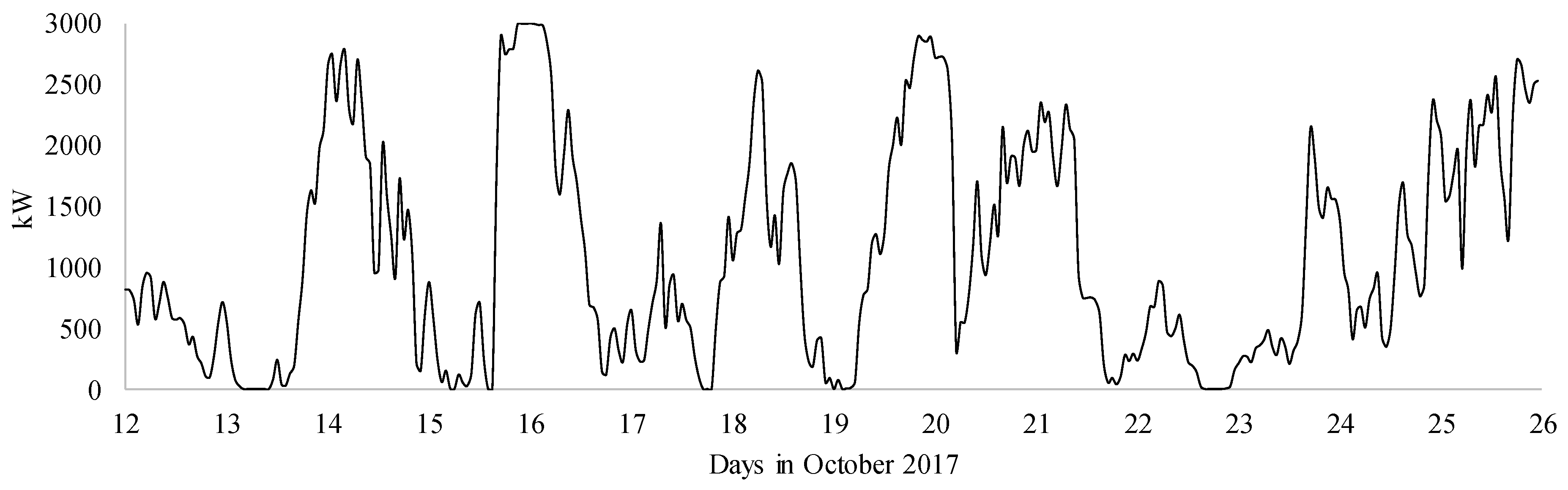
3.1. Experimental Data
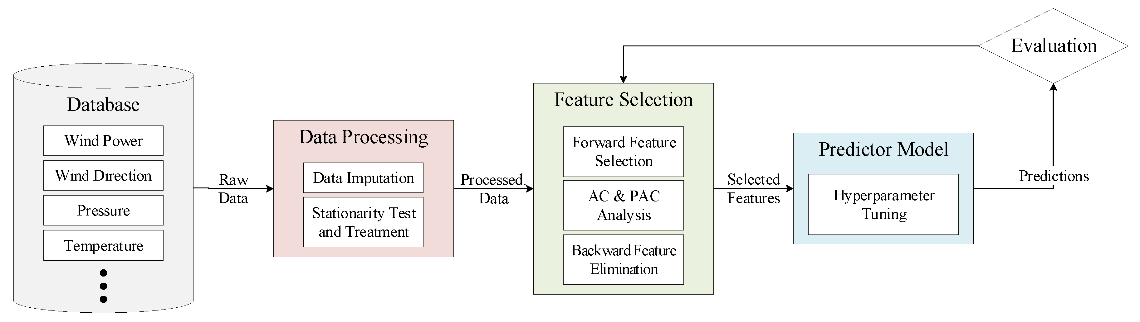
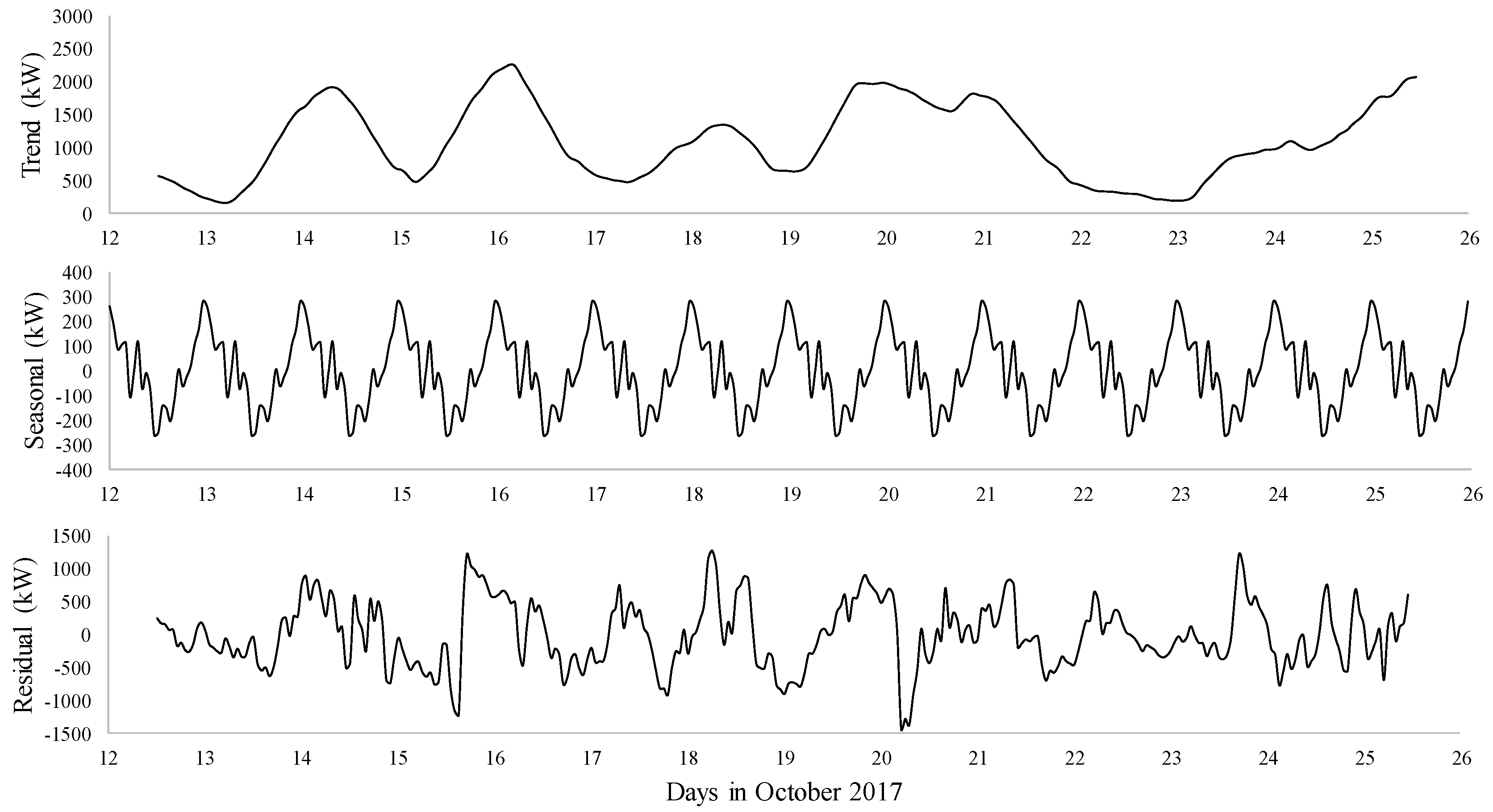
3.2. Data Processing
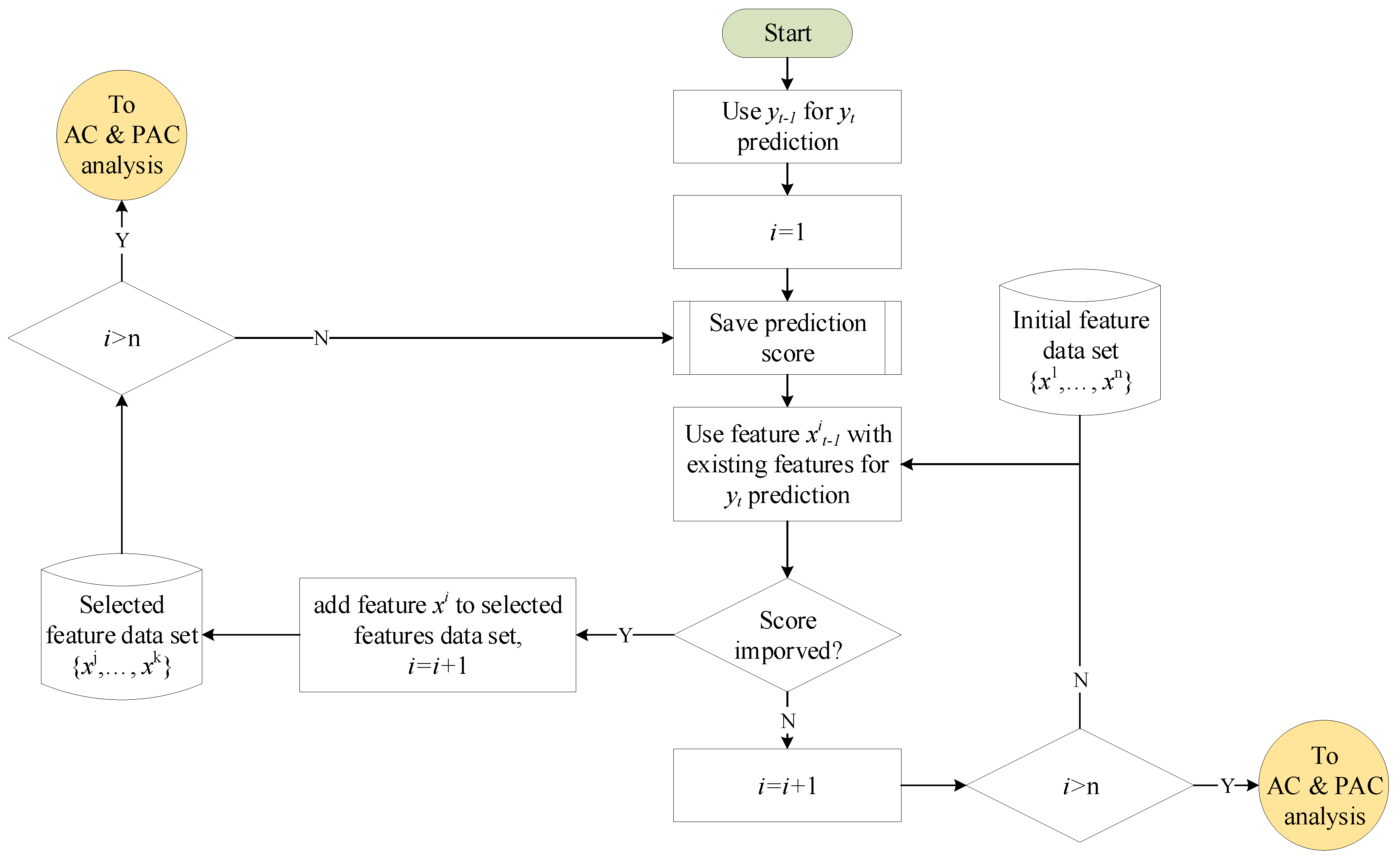
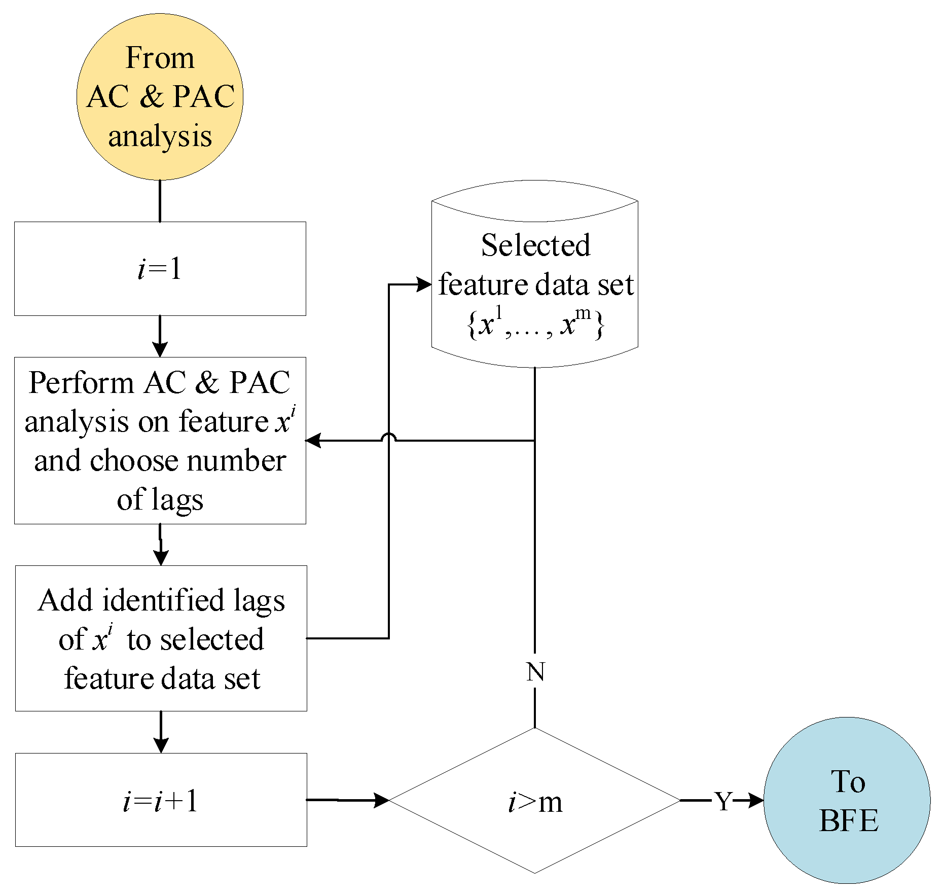
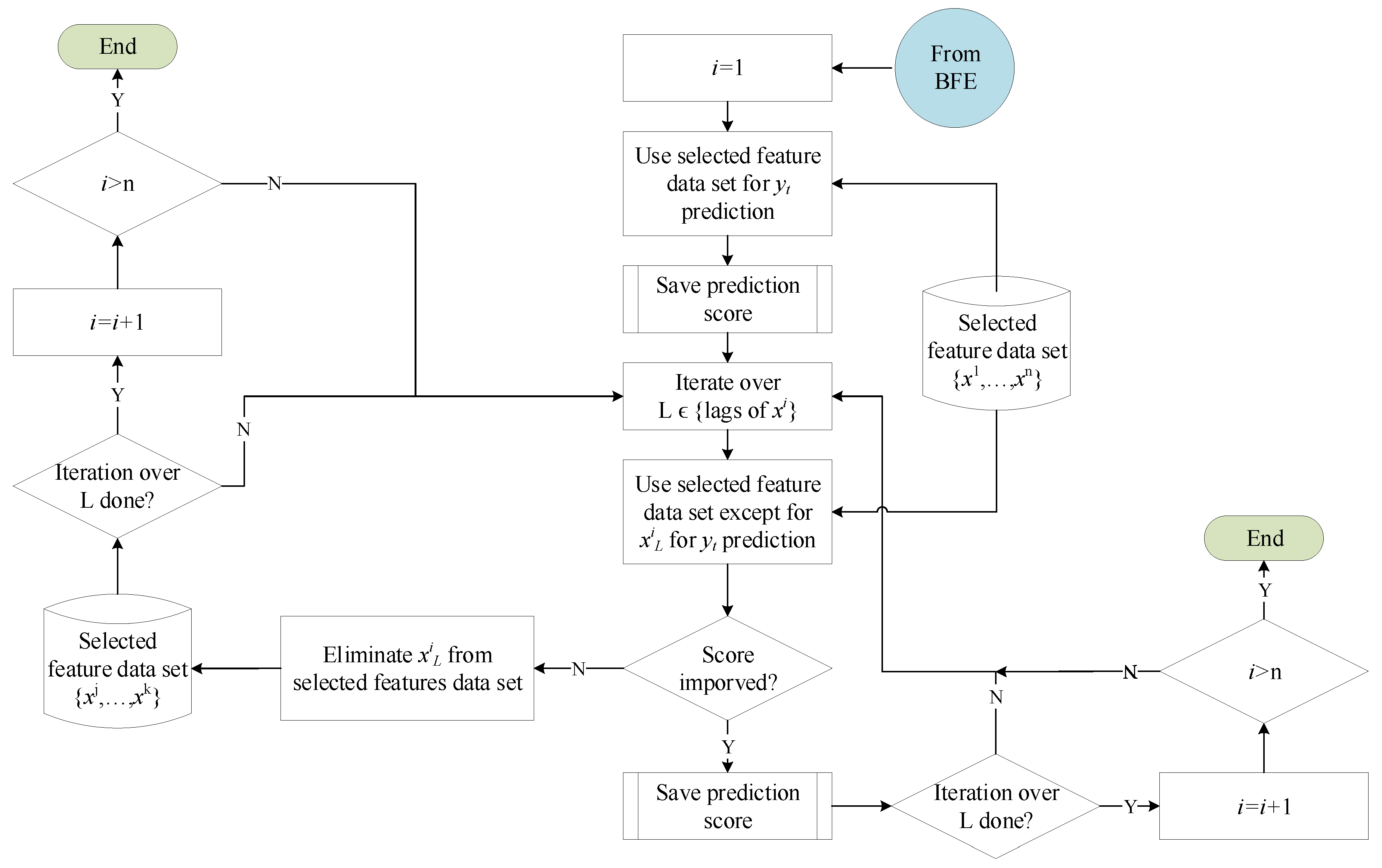
3.3. Feature Selection
3.4. Results
4. Data-Driven BESS Sizing
4.1. Battery Characteristics
4.2. Methodology
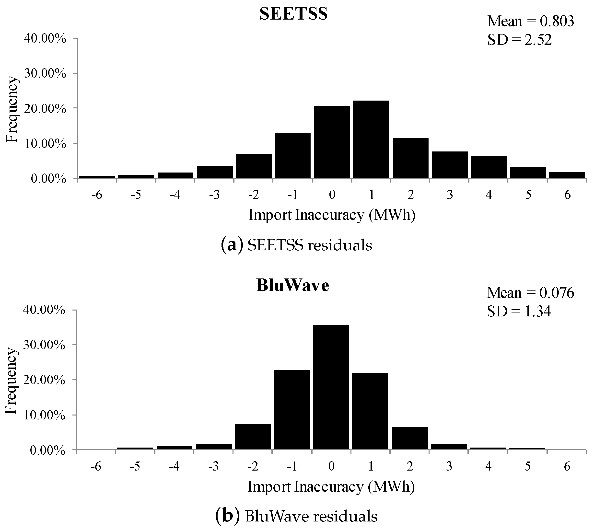
- Populate a set of import inaccuracies vector, , based on the results presented in Figure 11.
- Populate a set of BESS energy capacity, . For each element in , populate a set of C-rates, .
- For each element in and its corresponding elements in , calculate the charged and discharged energies for each element in . Calculate the savings by reducing investment cost from energy savings. Thus, for each simulation scenario , there exist s simulation scenarios .
- Calculate the final savings for each element in and its corresponding elements in by averaging the savings calculated for the elements in .
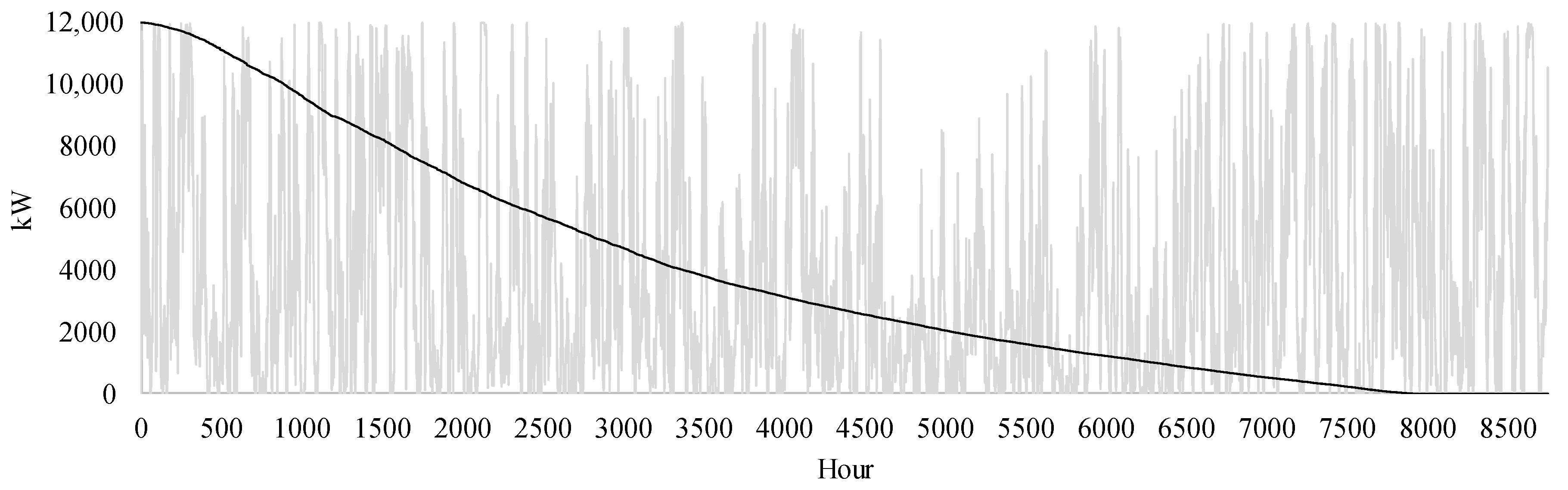
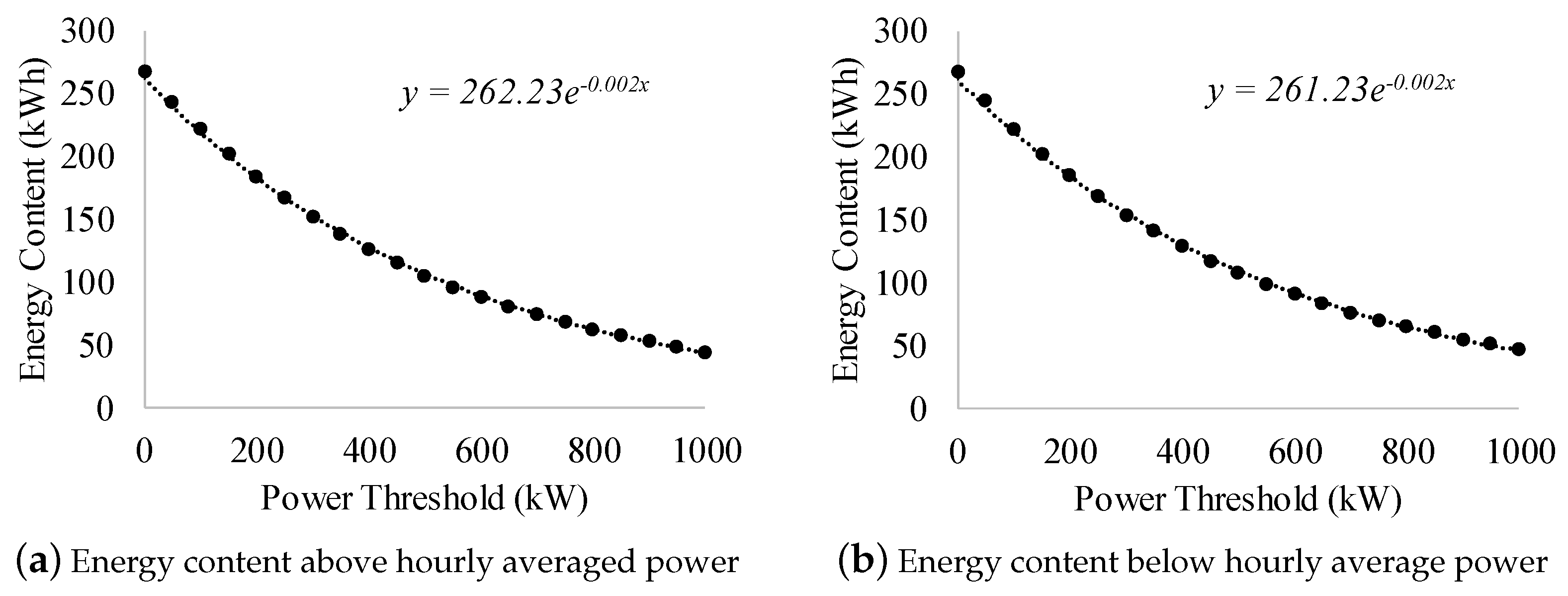
- Calculate the hourly averaged power.
- Populate a set of power threshholds. In this case, the power threshold ranges from 0–1000 kW with steps of 50 kW.
- Calculate the energy above and below the average required power for each power threshold.
- Calculate the average of calculated energies for each power threshold.
- Fit the appropriate trendline to the calculated average energy of power thresholds [52]. In this case, an exponential trendline is chosen based on the observed data. The trendline expression can be used to estimate the energy above and below the hourly average required power for a certain power threshold.
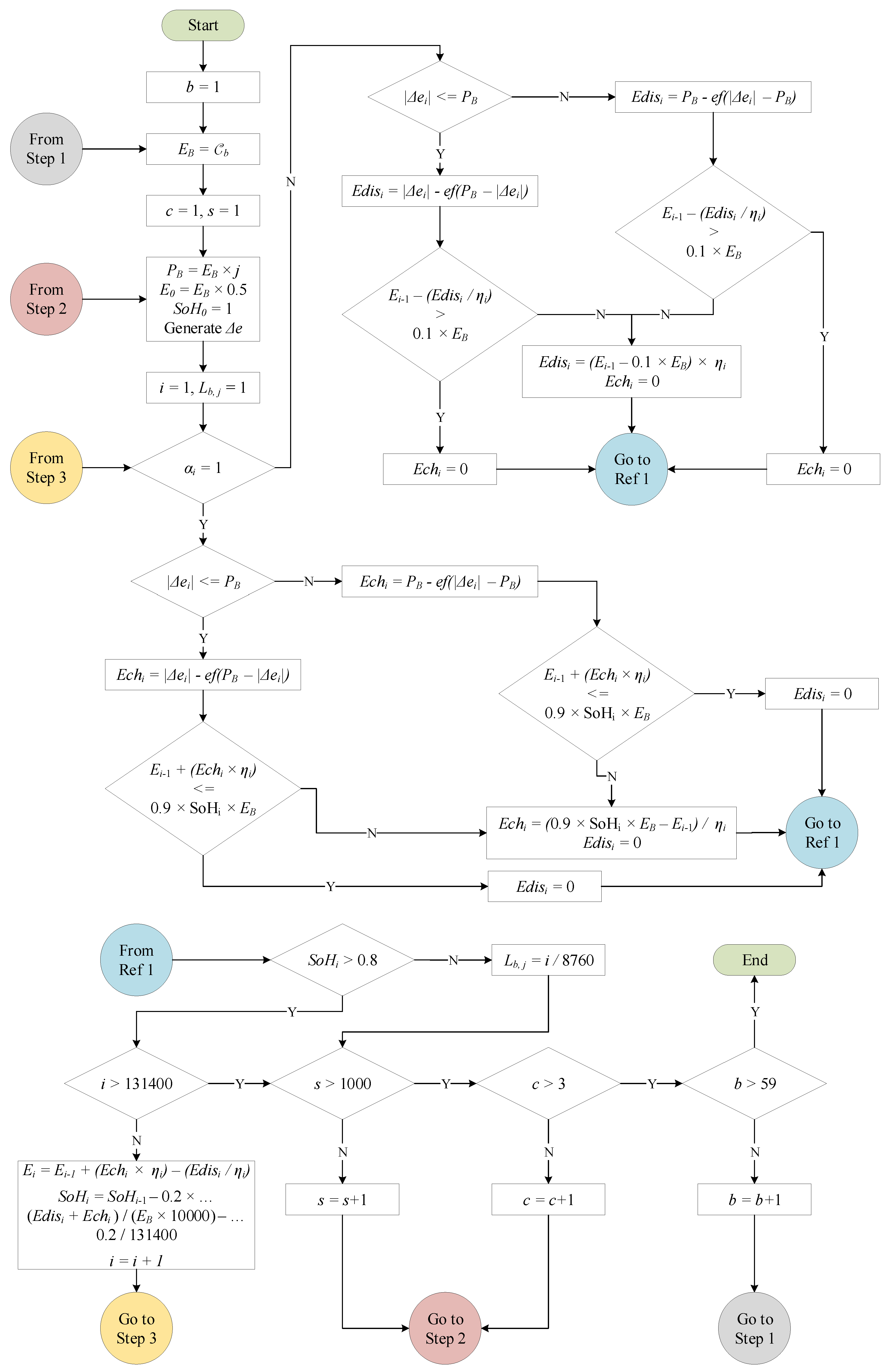
- = 1, i.e., there is surplus of energy .
- If Equation (13) is true, i.e., the average surplus power within the time interval does not exceed the battery power rating, go to step 3, otherwise go to step 6:
- Estimate BESS charged energy using Equation (14):
- If Equation (15) is true, i.e., the battery energy content at the end of the time interval does not exceed the maximum acceptable energy capacity, end the process and go to the next time step, otherwise go to step 5:
- Estimate the BESS charged energy using Equation (16); end the process and go to the next time step:
- Estimate BESS charged energy using Equation (17):
- If Equation (15) is true, end the process and go to the next time step, otherwise go to step 8.
- Estimate the charged energy using Equation (16); end the process and go to the next time step.
- = 0, i.e., there is deficit of energy .
- If Equation (13) is true, go to step 3, otherwise go to step 6.
- Estimate BESS charged energy using Equation (18):
- If Equation (19) is true, i.e., the battery energy content at the end of the time interval is not below the minimum acceptable energy capacity, end the process and go to the next time step, otherwise go to step 5:
- Estimate the BESS charged energy using Equation (20); end the process and go to the next time step:
- Estimate BESS charged energy using Equation (21):
- If Equation (19) is true, end the process and go to the next time step, otherwise go to step 8.
- Estimate the charged energy using Equation (20); end the process and go to the next time step.
5. Economics of the Wind-BESS System
5.1. Optimal BESS Capacity
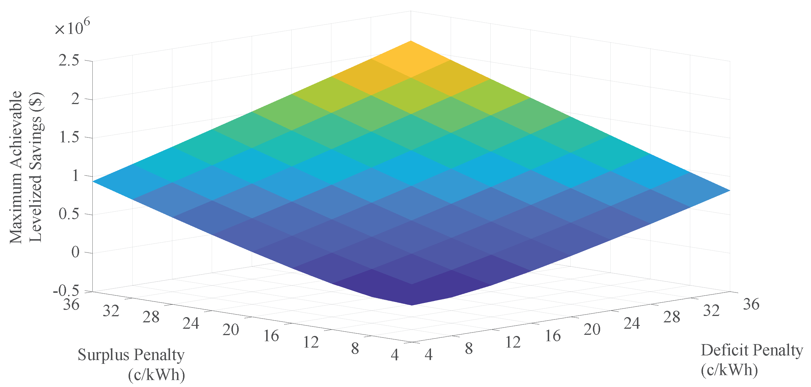
5.2. Highest Achievable Savings
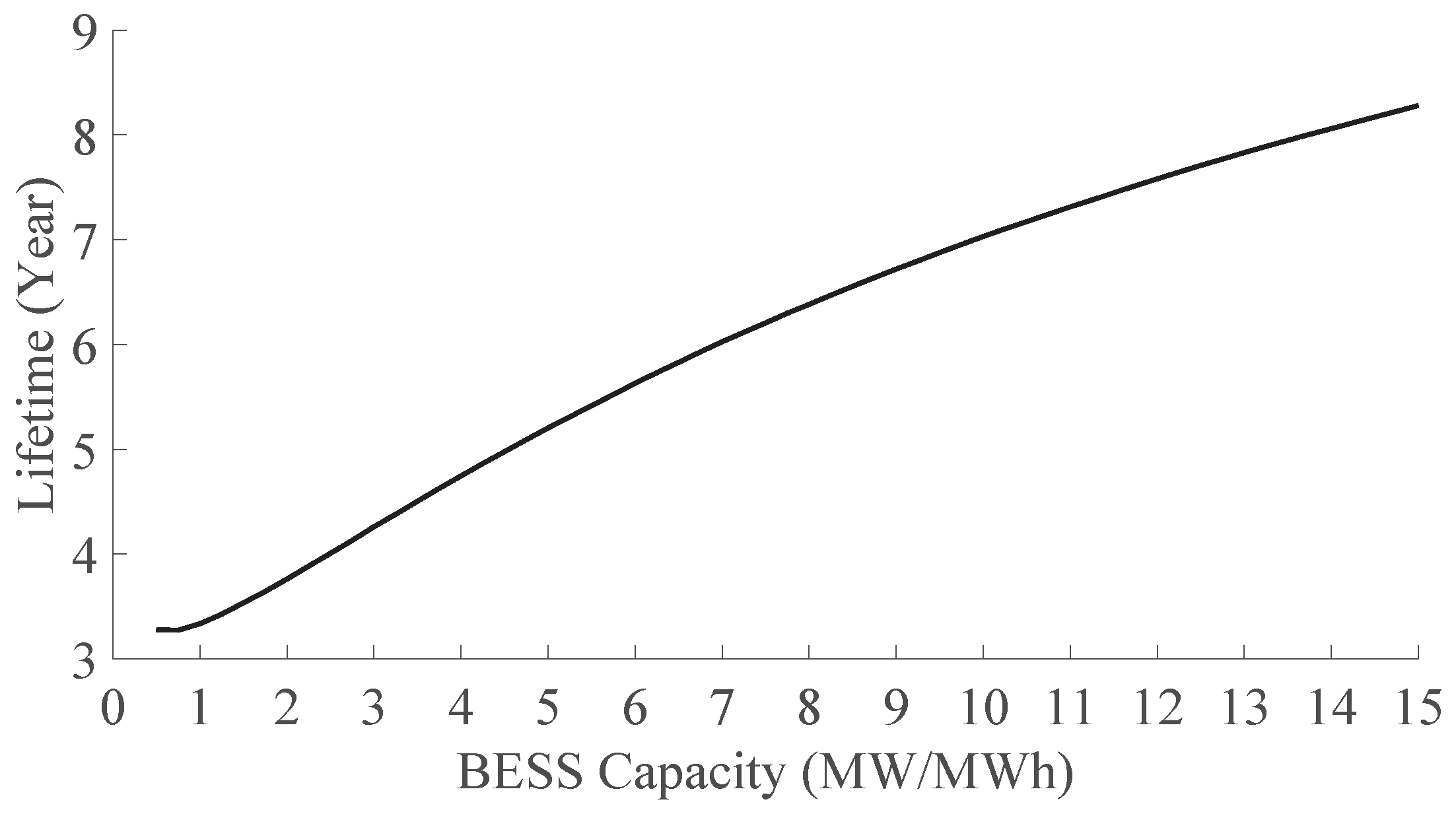
5.3. BESS Lifetime
5.4. Interpretation and Analysis
6. Conclusions
Funding
Acknowledgments
Conflicts of Interest
Abbreviations
| AC | Autocorrelation |
| ADF | Augmented Dickey–Fuller |
| AI | Artificial Intelligence |
| ARIMA | Autoregressive Integrated Moving Average |
| BESS | Battery Energy Storage Systems |
| BFE | Backward Feature Elimination |
| ESS | Energy Storage Systems |
| LIB | Lithium-Ion Battery |
| MAE | Mean Absolute Error |
| MOU | Memorandum of Understanding |
| NREL | National Renewable Energy Laboratory |
| NWP | Numerical Weather Prediction |
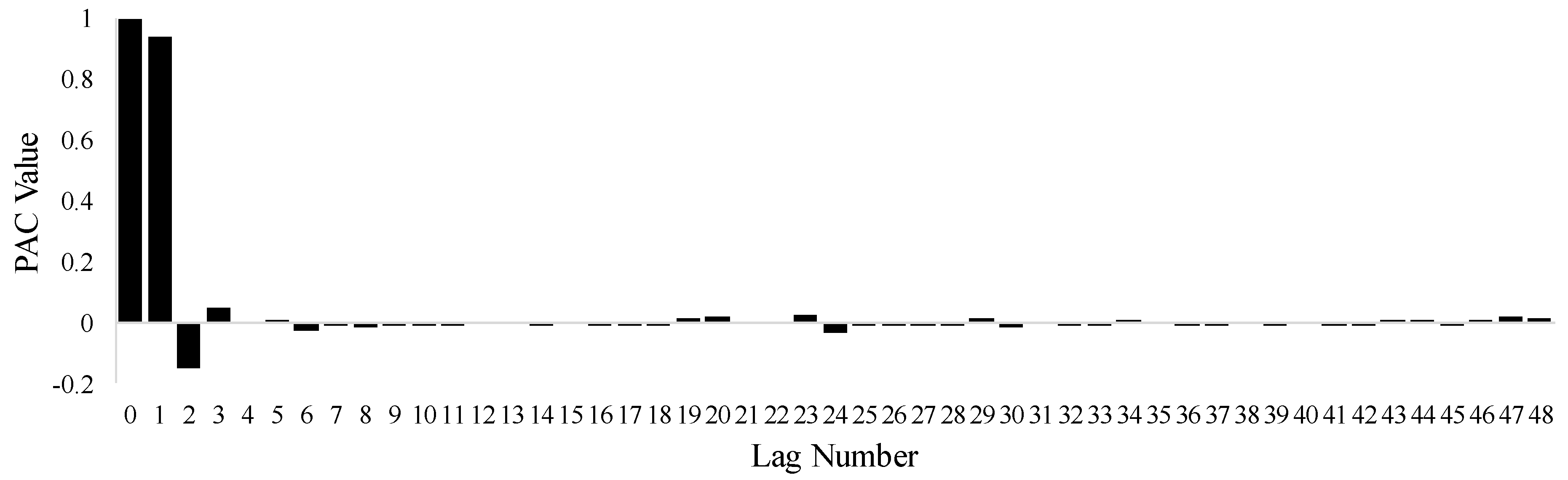
| PAC | Partial Autocorrelation |
| PEI | Prince Edward Island |
| RES | Renewable Energy Resources |
| SCADA | Supervisory Control and Data Acquisition |
| SEETSS | Summerside Electric Energy Transmission Scheduling System |
| SOH | State of Health |
| SVM | Support Vector Machine |
References
- Nanaki, E.A.; Xydis, G.A. Deployment of Renewable Energy Systems: Barriers, Challenges, and Opportunities. Adv. Renew. Energies Power Technol. 2018, 2, 207–229. [Google Scholar]
- Eftekharnejad, S.; Vittal, V.; Heydt, G.T.; Keel, B.; Loehr, J. Impact of increased penetration of photovoltaic generation on power systems. IEEE Trans. Power Syst. 2013, 28, 893–901. [Google Scholar] [CrossRef]
- Ulbig, A.; Borsche, T.S.; Andersson, G. Impact of Low Rotational Inertia on Power System Stability and Operation. IFAC Proc. Vol. 2014, 47, 7290–7297. [Google Scholar] [CrossRef] [Green Version]
- Wang, J.; Botterud, A.; Bessa, R.; Keko, H.; Carvalho, L.; Issicaba, D.; Sumaili, J.; Miranda, V. Wind Power Forecasting Uncertainty and Unit Commitment. Appl. Energy 2011, 88, 4014–4023. [Google Scholar] [CrossRef]
- Farrokhabadi, M.; Konig, S.; Canizares, C.A.; Bhattacharya, K.; Leibfried, T. Battery Energy Storage System Models for Microgrid Stability Analysis and Dynamic Simulation. IEEE Trans. Power Syst. 2018, 33, 2301–2312. [Google Scholar] [CrossRef]
- Hong, T.; Pinson, P.; Fan, S. Global Energy Forecasting Competition 2012. Int. J. Forecast. 2014, 30, 357–363. [Google Scholar] [CrossRef]
- Marugan, A.P.; Marquez, F.P.G.; Perez, J.M.P.; Ruiz-Hernandez, D. A Survey of Artificial Neural Network in Wind Energy Systems. Appl. Energy 2018, 228, 1822–1836. [Google Scholar] [CrossRef]
- Ordinao, J.A.G.; Waczowicz, S.; Hegenmeyer, V.; Mikut, R. Energy Forecasting Tools and Services. WIREs Data Min. Knowl. Discov. 2018, 8, 1–20. [Google Scholar]
- Wong, S.; Gaudet, G.; Proulx, L. Capturing Wind with Thermal Energy Storage-Summerside’s Smart Grid Approach. IEEE Power Energy Technol. Syst. J. 2017, 4, 115–124. [Google Scholar] [CrossRef]
- Mi, Z.; Jia, Y.; Wang, J.; Zheng, X. Optimal Scheduling Strategies of Distributed Energy Storage Aggregator in Energy and Reserve Markets Considering Wind Power Uncertainties. Energies 2018, 11, 1242. [Google Scholar] [CrossRef]
- Stein, K.; Tun, M.; Musser, K.; Rocheleau, R. Evaluation of a 1 MW, 250 kW-hr Battery Energy Storage System for Grid Services for the Island of Hawaii. Energies 2018, 11, 3367. [Google Scholar] [CrossRef]
- Feng, C.; Cui, M.; Hodge, B.; Zhang, J. A data-driven multi-model methodology with deep feature selection for short-term wind forecasting. Appl. Energy 2017, 190, 1245–1257. [Google Scholar] [CrossRef] [Green Version]
- Richardson, L.F. Weather Prediction by Numerical Process; Cambridge University Press: New York, NY, USA, 2007. [Google Scholar]
- Ma, L.; Luan, S.; Jiang, C.; Liu, H.; Zhang, Y. A Review on the Forecasting of Wind Speed and Generated Power. Renew. Sustain. Energy Rev. 2009, 3, 915–920. [Google Scholar]
- Al-Yahyai, S.; Charabi, Y.; Gastli, A. Review of the Use of Numerical Weather Prediction (NWP) Models for Wind Energy Assessment. Renew. Sustain. Energy Rev. 2010, 14, 3192–3198. [Google Scholar] [CrossRef]
- Cadenas, E.; Rivera, W.; Campos-Amezcua, R.; Heard, C. Wind Speed Prediction Using a Univariate ARIMA Model and a Multivariate NARX Model. Energies 2016, 9, 109. [Google Scholar] [CrossRef]
- Poncela, M.; Poncela, P.; Peran, J. Automatic Tuning of Kalman Filters by Maximum Likelihood Methods for Wind Energy Forecasting. Appl. Energy 2013, 108, 349–362. [Google Scholar] [CrossRef]
- Santamaria-Bonfil, G.; Reyes-Ballesteros, A.; Gershenson, C. Wind Speed Forecasting for Wind Farms: A Method Based on Support Vector Regression. Renew. Energy 2016, 56, 790–806. [Google Scholar] [CrossRef]
- Chang, G.; Lu, H.; Chang, Y.; Lee, Y. An Improved Neural Network-based Approach for Short-Term Wind Speed and Power Forecast. Renew. Energy 2017, 105, 301–311. [Google Scholar] [CrossRef]
- Doucoure, B.; Agbossou, K.; Cardenas, A. Time Series Prediction Using Artificial Wavelet Neural Network and Multi-Resolution Analysis: Application to Wind Speed Data. Renew. Energy 2016, 92, 202–211. [Google Scholar] [CrossRef]
- Chow, T.; Li, S.; Fang, Y. A Real-Time Learning Control Approach for Nonlinear Continuous-Time System Using Recurrent Neural Networks. IEEE Trans. Ind. Electr. 2000, 47, 478–486. [Google Scholar] [CrossRef]
- Sanchez, I. Adaptive Combination of Forecasts with Application to Wind Energy. Int. J. Forecast. 2008, 24, 679–693. [Google Scholar] [CrossRef]
- Delille, G.; Franois, B.; Malarange, G. Dynamic Frequency Control Support by Energy Storage to Reduce the Impact of Wind and Solar Generation on Isolated Power System’s Inertia. IEEE Trans. Sustain. Energy 2012, 3, 931–939. [Google Scholar] [CrossRef]
- Farrokhabadi, M.; Solanki, B.V.; Canizares, C.A.; Bhattacharya, K.; Koenig, S.; Sauter, P.S.; Leibfried, T.; Hohmann, S. Energy Storage in Microgrids: Compensating for Generation and Demand Fluctuations While Providing Ancillary Services. IEEE Power Energy Mag. 2017, 15, 81–91. [Google Scholar] [CrossRef]
- Lo, C.; Anderson, M.A. Economic Dispatch and Optimal Sizing of Battery Energy Storage Systems in Utility Load-Leveling Operations. IEEE Trans. Energy Convers. 1999, 14, 824–829. [Google Scholar] [CrossRef]
- Nottrott, A.; Klessl, J.; Washom, B. Energy Dispatch Schedule Optimization and Cost Benefit Analysis for Grid-Connected, Photovoltaic-Battery Storage Systems. Renew. Energy 2013, 55, 230–240. [Google Scholar] [CrossRef]
- Bathurst, G.; Strbac, G. Value of Combining Energy Storage and Wind in Short-Term Energy and Balancing Markets. Electr. Power Syst. Res. 2003, 67, 1–8. [Google Scholar] [CrossRef]
- Arefi, A.; Shahnia, F.; Ledwich, G. Electric Distribution Network Management and Control; Springer: Singapore, 2018. [Google Scholar]
- Hesse, H.C.; Martins, R.; Musilek, P.; Naumann, M.; Truong, C.N.; Jossen, A. Economic Optimization of Component Sizing for Residential Battery Storage Systems. Energies 2017, 10, 835. [Google Scholar] [CrossRef]
- Ying, Y.; Bremnera, S.; Menictasb, C.; Kaya, M. Battery Energy Storage System Size Determination in Renewable Energy Systems: A Review. Renew. Sustain. Energy Rev. 2018, 91, 109–125. [Google Scholar] [CrossRef]
- Wu, J.; Zhang, B.; Li, H.; Li, Z.; Chen, Y.; Miao, X. Statistical Distribution for Wind Power Forecast Error and its Application to Determine Optimal Size of Energy Storage System. Int. J. Electr. Power Energy Syst. 2014, 55, 100–107. [Google Scholar] [CrossRef]
- Tan, C.W.; Green, T.C.; Hernandez-Aramburo, C.A. A Stochastic Method for Battery Sizing with Uninterruptible Power and Demand Shift Capabilities in PV (photovoltaic) systems. Energy 2010, 35, 5082–5092. [Google Scholar] [CrossRef]
- Nguyen, T.A.; Crow, M.L.; Elmore, A.C. Optimal Sizing of a Vanadium Redox Battery System for Microgrid Systems. IEEE Trans. Sustain. Energy 2015, 6, 729–737. [Google Scholar] [CrossRef]
- Bahramirad, S.; Reder, W.; Khodaei, A. Reliability-Constrained Optimal Sizing of Energy Storage System in a Microgrid. IEEE Trans. Smart Grid 2012, 3, 2056–2062. [Google Scholar] [CrossRef]
- Fossati, J.P.; Galarza, A.; Martin-Villate, A.; Fontan, L. A Method for Optimal Sizing Energy Storage Systems for Microgrids. Renew. Energy 2015, 77, 539–549. [Google Scholar] [CrossRef]
- Saboori, H.; Hemmati, R.; Jirdehi, M.A. Reliability Improvement in Radial Electrical Distribution Network by Optimal Planning of Energy Storage Systems. Energy 2015, 93, 2299–2312. [Google Scholar] [CrossRef]
- Summerside, Prince Edward Island. Available online: https://en.wikipedia.org/wiki/Summerside,_Prince_Edward_Island (accessed on 9 February 2019).
- Brockwell, P.J.; Davis, R.A. Introduction to Time Series and Forecasting; Springer: Cham, Switzerland, 2016. [Google Scholar]
- Virili, F.; Freisleben, B. Nonstationarity and Data Preprocessing for Neural Network Predictions of an Economic Time Series. In Proceedings of the IEEE-INNS-ENNS International Joint Conference on Neural Networks, Como, Italy, 27 July 2000; pp. 129–134. [Google Scholar]
- Nelson, C.R.; Plosser, C.R. Trends and Random Walks in Macroeconmic Time Series: Some Evidence and Implications. J. Monet. Econ. 1982, 10, 139–162. [Google Scholar] [CrossRef]
- Makridakis, S.; Wheelwright, S.; Hyndman, R. Forecasting: Methods and Applications; Wiley: New York, NY, USA, 1997. [Google Scholar]
- Flores, J.H.F.; Engel, P.M.; Pinto, R.C. Autocorrelation and Partial Autocorrelation Functions to Improve Neural Networks Models on Univariate Time Series Forecasting. In Proceedings of the 2012 International Joint Conference on Neural Networks (IJCNN), Brisbane, QLD, Australia, 10–15 June 2012; pp. 1–8. [Google Scholar]
- Bao, Y.; Zhitao, L. A Fast Grid Search Method in Support Vector Regression Forecasting Time Series. In Proceedings of the International Conference on Intelligent Data Engineering and Automated Learning (IDEAL), Burgos, Spain, 20–23 September 2006; pp. 504–511. [Google Scholar]
- Martins, R.; Hesse, H.C.; Jungbauer, J.; Vorbuchner, T.; Musilek, P. Optimal Component Sizing for Peak Shaving in Battery Energy Storage System for Industrial Applications. Energies 2018, 11, 2048. [Google Scholar] [CrossRef]
- Fu, R.; Remo, T.; Margolis, R. 2018 U.S. Utility-Scale Photovoltaics-Plus-Energy Storage System Costs Benchmark; Technical Report TP-6A20-71714; National Renewable Energy Laboratory (NREL): Denver, CO, USA, 2018.
- Few, S.; Schmidt, O.; Offer, G.J.; Brandon, N.; Nelson, J.; Gambhir, A. Prospective Improvements in Cost and Cycle Life of Off-Grid Lithium-Ion Battery Packs: An Analysis Informed by Expert Elicitations. Energy Policy 2018, 114, 578–590. [Google Scholar] [CrossRef]
- Vetter, J.; Novak, P.; Wagner, M.R.; Veit, C.; Moller, K.C.; Besenhard, J.O.; Winter, M.; Wohlfahrt-Mehrens, M.; Vogler, C.; Hammouche, A. Ageing Mechanisms in Lithium-Ion Batteries. J. Power Sources 2005, 147, 269–328. [Google Scholar] [CrossRef]
- Battke, B.; Schmidt, T.S.; Grosspietsch, D.; Hoffmann, V.H. A Review and Probabilistic Model of Lifecycle Costs of Stationary Batteries in Multiple Applications. Renew. Sustain. Energy Rev. 2013, 25, 240–250. [Google Scholar] [CrossRef]
- Barre, A.; Deguilhem, B.; Grolleau, S.; Gerard, M.; Suard, F.; Riu, D. A Review on Lithium-Ion Battery Ageing Mechanisms and Estimations for Automotive Applications. J. Power Sources 2013, 241, 680–689. [Google Scholar] [CrossRef]
- Hesse, H.C.; Schimpe, M.; Kucevic, D.; Jossen, A. Lithium-Ion Battery Storage for the Grid—A Review of Stationary Battery Storage System Design Tailored for Applications in Modern Power Grids. Energies 2017, 10, 2107. [Google Scholar] [CrossRef]
- Rubinstein, R.Y.; Kroese, D.P. Simulation and the Monte Carlo Method; John Wiley & Sons: Hoboken, NJ, USA, 2016. [Google Scholar]
- Guest, P.G. Numerical Methods of Curve Fitting; Cambridge University Press: Cambridge, UK, 2013. [Google Scholar]


| Number of Data Points | Resolution | Number of Features | Source | |
|---|---|---|---|---|
| Dataset 1 | 17,568 | Hourly | 7 | Summerside Electric |
| Dataset 2 | 52,560 | 10-min | 98 | Summerside Electric |
| Dataset 3 | 17,568 | Hourly | 18 | Environment and Climate Change Canada |
| Wind MAE (kWh) | Load MAE (kWh) | Import MAE (kWh) | |
|---|---|---|---|
| Summerside | 1383 | 800 | 1872 |
| BluWave | 851 | 332 | 976 |
| Improvement | 62% | 58% | 48% |
| Cost ($/kWh) | 450 | 600 | 750 |
| Symbol | Type | Description | Unit |
|---|---|---|---|
| Set | BESS energy capacities | ||
| Set | BESS C-rates | ||
| Set | Import error scenarios | ||
| Set | time-steps | ||
| b | Index | BESS energy capacity | |
| c | Index | BESS C-rate | |
| i | Index | time-step | |
| s | Index | Import error scenario | |
| Parameter | Binary parameter indicating energy surplus during time-step i | ||
| Parameter | One-way converter efficiency | % | |
| Parameter | Import inaccuracy at time-step i | MWh | |
| Parameter | Time interval length | 1 h | |
| Parameter | BESS nominal energy capacity for simulation scenario b | MWh | |
| Parameter | BESS nominal Power capacity for simulation scenarios | MW | |
| Variable | BESS energy at the end of time-step i for simulation scenario | MWh | |
| Variable | BESS charged energy during time-step i for simulation scenario | MWh | |
| Variable | BESS discharged energy during time-step i for simulation scenario | MWh | |
| Variable | BESS end of life for simulation scenario | ||
| Variable | BESS state of health at the end of time-step i for simulation scenario |
| \ | 4 | 8 | 12 | 16 | 20 | 24 | 28 | 32 | 36 |
|---|---|---|---|---|---|---|---|---|---|
| 4 | 0.5 | 1 | 2.75 | 4 | 5.25 | 5.75 | 6.5 | 7.5 | 8 |
| 8 | 1.25 | 3 | 4.25 | 5.25 | 5.75 | 6.5 | 7.5 | 8.25 | 9.25 |
| 12 | 3.25 | 4.5 | 5.25 | 5.75 | 7.25 | 8 | 8.25 | 9.25 | 9.25 |
| 16 | 4.5 | 5.5 | 6.5 | 7.5 | 8 | 8.5 | 9.25 | 9.25 | 10.75 |
| 20 | 5.5 | 6.5 | 7.5 | 8 | 8.5 | 9.25 | 10.5 | 10.75 | 11.25 |
| 24 | 6.5 | 7.5 | 8 | 8.5 | 9.25 | 10.5 | 11.25 | 11.25 | 11.25 |
| 28 | 7.5 | 8 | 8.75 | 9.25 | 10.5 | 11.25 | 11.25 | 11.25 | 12 |
| 32 | 8 | 9.25 | 9.25 | 10.75 | 11.25 | 11.25 | 11.25 | 12 | 12.75 |
| 36 | 9.25 | 9.25 | 10.75 | 11.25 | 11.25 | 11.25 | 12 | 14 | 14 |
| \ | 4 | 8 | 12 | 16 | 20 | 24 | 28 | 32 | 36 |
|---|---|---|---|---|---|---|---|---|---|
| 4 | −0.021 | 0.003 | 0.076 | 0.179 | 0.295 | 0.419 | 0.547 | 0.681 | 0.817 |
| 8 | 0.008 | 0.086 | 0.191 | 0.308 | 0.432 | 0.561 | 0.695 | 0.837 | 0.971 |
| 12 | 0.097 | 0.203 | 0.322 | 0.446 | 0.575 | 0.710 | 0.847 | 0.987 | 1.128 |
| 16 | 0.216 | 0.335 | 0.460 | 0.590 | 0.725 | 0.862 | 1.002 | 1.143 | 1.288 |
| 20 | 0.348 | 0.474 | 0.604 | 0.739 | 0.876 | 1.017 | 1.159 | 1.304 | 1.451 |
| 24 | 0.4875 | 0.619 | 0.754 | 0.891 | 1.032 | 1.174 | 1.320 | 1.467 | 1.614 |
| 28 | 0.633 | 0.769 | 0.906 | 1.048 | 1.190 | 1.336 | 1.483 | 1.630 | 1.777 |
| 32 | 0.784 | 0.922 | 1.063 | 1.206 | 1.352 | 1.499 | 1.646 | 1.793 | 1.943 |
| 36 | 0.937 | 1.078 | 1.221 | 1.368 | 1.515 | 1.662 | 1.809 | 1.959 | 2.112 |
| \ | 4 | 8 | 12 | 16 | 20 | 24 | 28 | 32 | 36 |
|---|---|---|---|---|---|---|---|---|---|
| 4 | 2.5 | 4.5 | 10 | 12.75 | 15 | 15.75 | 16.75 | 18.25 | 19 |
| 8 | 5.5 | 10.75 | 13.25 | 15 | 15.75 | 16.75 | 18.25 | 19.25 | 20.5 |
| 12 | 11.25 | 13.75 | 15 | 15.75 | 18 | 19 | 19.25 | 20.5 | 20.5 |
| 16 | 13.75 | 15.25 | 16.75 | 18.25 | 19 | 19.5 | 20.5 | 20.5 | 22.25 |
| 20 | 15.25 | 16.75 | 18.25 | 19 | 19.5 | 20.5 | 22 | 22.25 | 23 |
| 24 | 16.75 | 18.25 | 19 | 19.5 | 20.5 | 22 | 23 | 23 | 23 |
| 28 | 18.25 | 19 | 20 | 20.5 | 22 | 23 | 23 | 23 | 23.75 |
| 32 | 19 | 20.5 | 20.5 | 22.25 | 23 | 23 | 23 | 23.75 | 24.75 |
| 36 | 20.5 | 20.5 | 22.25 | 23 | 23 | 23 | 23.75 | 26.25 | 26.25 |
© 2019 by the author. Licensee MDPI, Basel, Switzerland. This article is an open access article distributed under the terms and conditions of the Creative Commons Attribution (CC BY) license (http://creativecommons.org/licenses/by/4.0/).
Share and Cite
Farrokhabadi, M. Data-Driven Mitigation of Energy Scheduling Inaccuracy in Renewable-Penetrated Grids: Summerside Electric Use Case. Energies 2019, 12, 2228. https://doi.org/10.3390/en12122228
Farrokhabadi M. Data-Driven Mitigation of Energy Scheduling Inaccuracy in Renewable-Penetrated Grids: Summerside Electric Use Case. Energies. 2019; 12(12):2228. https://doi.org/10.3390/en12122228
Chicago/Turabian StyleFarrokhabadi, Mostafa. 2019. "Data-Driven Mitigation of Energy Scheduling Inaccuracy in Renewable-Penetrated Grids: Summerside Electric Use Case" Energies 12, no. 12: 2228. https://doi.org/10.3390/en12122228
APA StyleFarrokhabadi, M. (2019). Data-Driven Mitigation of Energy Scheduling Inaccuracy in Renewable-Penetrated Grids: Summerside Electric Use Case. Energies, 12(12), 2228. https://doi.org/10.3390/en12122228