Article

Data-Driven Mitigation of Energy Scheduling Inaccuracy in Renewable-Penetrated Grids: Summerside Electric Use Case

by
Mostafa Farrokhabadi
BluWave-ai, Ottawa, ON K2L 1T9, Canada
Energies 2019, 12(12), 2228; https://doi.org/10.3390/en12122228
Submission received: 1 April 2019 / Revised: 17 May 2019 / Accepted: 28 May 2019 / Published: 12 June 2019
(This article belongs to the Special Issue Grid-Scale Energy Storage Management)

Abstract

:
This paper presents findings on mitigating the negative impact of renewable energy resources variability on the energy scheduling problem, in particular for island grids and microgrids. The methods and findings presented in this paper are twofold. First, data obtained from the City of Summerside in the province of Prince Edward Island, Canada, is leveraged to demonstrate the effectiveness of state-of-the-art time series predictors in mitigating energy scheduling inaccuracy. Second, the outcome of the time series prediction analysis is used to propose a novel data-driven battery energy storage system (BESS) sizing study for energy scheduling purposes. The proposed probabilistic method accounts for intra-interval variations of generation and demand, thus mitigating the trade-off between time resolution of the problem formulation and the solution accuracy. In addition, as part of the sizing study, a BESS management strategy is proposed to minimize energy scheduling inaccuracies, and is then used to obtain the optimal BESS size. Finally, the paper presents quantitative analyses of the impact of both the energy predictors and the BESS on the supplied energy cost using the actual data of the Summerside Electric grid. The paper reveals the significant potential for reducing energy cost in renewable-penetrated grids and microgrids through state-of-the-art predictors combined with applications of properly-sized energy storage systems.

1. Introduction

Driven by the need for cheap, sustainable, and clean sources of energy, renewable energy resources (RES), in particular wind and solar energies are being deployed increasingly across many countries [1]. High penetration of wind and solar energies poses some operational challenges, affecting system stability, reliability, and economics [2]. These challenges can be categorized into two main groups: (i) those associated with the decrease of system inertia [3]; and (ii) those associated with the intrinsic variability and uncertainty of RES [4]. In particular, island grids and microgrids, where RES penetration tends to be high, are more prone to negative impacts of RES variability and low system inertia [5]. In view of these challenges, numerous techniques have been proposed in the literature to alleviate the impact of high RES penetration. These include methods pertaining to enhancing the prediction accuracy of RES [6,7,8] and techniques pertaining to the use of energy storage systems (ESS) [9,10], in particular battery energy storage systems (BESS) [11].
RES prediction techniques are categorized into three major methods [12]: (i) numerical weather prediction (NWP) models [13]; (ii) data-driven approaches [6]; and (iii) hybrid physical and statistical models [14]. NWP models are based on atmospheric science, utilizing differential equations derived from physical laws, in particular the first law of thermodynamics [15]. These are difficult to construct and are usually used for long-time forecasting, as they exhibit a poor performance for short-term prediction. In addition, NWP models need both meteorological and topological information which adds to the complexity of their operation. On the other hand, statistical models ingest historical data to predict future RES output typically for short time-intervals ahead. Statistical techniques can be mainly categorized into linear and nonlinear methods. Amongst the linear models, autoregressive integrated moving average models (ARIMA) [16], Kalman Filter [17], and support vector machines (SVM) [18] are the most popular techniques. Nonlinear models include neural network approaches such as multi-layer perceptrons and recurrent neural networks [19,20,21]. Finally, hybrid models include approaches that use NWP-based predictions as part of the input for statistical techniques [22].
ESS have two main applications in renewable-penetrated grids and microgrids: (i) to enhance system dynamic performance [11,23]; and (ii) to shift the RES output to reduce energy cost and emissions [24]. The latter application is the focus of this paper. For example, a multi-pass dynamic programming technique is proposed in [25] for optimal dispatch of BESS in a utility-scale grid. A linear programming model is formulated in [26] for peak net load management and demand charge minimization in a grid-connected PhotoVoltaic (PV)-BESS hybrid.
A price-based method is introduced in [27] to calculate the optimal dispatch of ESS considering short-term power exchange and expected imbalance penalties of a wind farm in a utility-scale grid. A cooperative stochastic optimal energy scheduling technique is discussed for a grid of microgrids in Chapter 9 of [28]; the method is based on the probability distribution of RES forecasting error and is shown to yield superior results compared to centralized techniques. These methods, along with numerous other techniques discussed in the literature, demonstrate the positive impact of ESS on economics of renewable-penetrated grids. However, BESS high investment cost and mediocre life cycle remain a major concern for grid operators, highlighting the significance of proper power and energy sizing [29].
Several techniques have been proposed in the literature for BESS sizing for a variety of applications [30]. These can be generally classified into three main categories: (i) analytical methods [31,32]; (ii) linear programming methods [33,34]; and (iii) nonlinear heuristic methods [35,36]. Analytical methods perform a series of simulations on varying variables of interest, in this case BESS power and energy capacity, to calculate the key performance metrics. The variables that yield highest performance metrics are selected as optimal. Analytical methods are usually amongst the most effective techniques given their flexibility for performance criteria and operational constraints. However, these methods can be computationally intensive depending on the number of simulations and time resolution [30]. Linear programming optimization methods formulate an explicit objective function intended to maximize the performance metrics. While these methods are computationally efficient and relatively easy to solve, they cannot account for nonlinear elements of BESS sizing problem, such as cycling aging. Finally, nonlinear heuristics methods can account for nonlinear constraints of optimization; however, they may converge to non-optimal or locally optimal solutions. On top of the aforementioned method-specific drawbacks, all of these methods suffer from the trade-off between time resolution and results accuracy. This issue will be further discussed in Section 4.
Considering the aforementioned discussion, this paper aims to reveal the potential to improve the economics of renewable-penetrated grids through mitigation of RES variability, particularly in the context of energy scheduling. Thus, the City of Summerside data from 2016 to 2018 is leveraged to reveal the significant potential for reducing energy cost in such systems. Located in Prince Edward Island (PEI), Canada, Summerside is the second largest city in the province and operates the only municipally-owned electric utility in PEI with a peak load of 28 MW [37]. Prior to 2009, the city imported dominant portion of electrical energy from NB Power, with the rest being supplied by local diesel generators. Since 2009, the city has installed 12 MW of wind turbine capacity, introducing Canada’s first municipally owned and operated wind farm [37]. Thus, in 2017, around 25% of the 137.5 TWh electrical demand was met by the wind farm; the rest was mostly imported from NB Power.
Summerside Electric imports energy from NB power in hourly intervals and the power must be scheduled 20 min ahead for the next interval. Thus, the city pays a commitment rate for the scheduled power. However, the intra-interval surplus of power is exported to NB power at a real-time rate lower than the commitment rate, and the deficit is imported at a rate much higher than the commitment rate. As a result, the accuracy of scheduled import plays a significant role in the overall price of imported power from NB power. With a wind power penetration as high as 100%, wind variations have a significant impact on the Summerside Electric power exchange with NB power. Thus, in 2018, Summerside Electric signed a memorandum of understanding (MOU) with BluWave-ai to enhance the energy import scheduling and control.
The work presented here shares some findings of the collaboration between BluWave-ai and Summerside Electric, and also proposes a novel data-driven approach for BESS sizing for energy scheduling applications. The discussion, methods, and findings presented in this paper are twofold. First, actual data is leveraged to demonstrate the effectiveness of state-of-the-art time series energy predictors in mitigating energy scheduling inaccuracies. Second, the outcome of the time series prediction analysis is used to propose a novel BESS sizing study for energy scheduling purposes. Considering the aforementioned drawbacks of current BESS sizing approaches, the proposed probabilistic method accounts for intra-interval variations of generation and demand, thus mitigating the trade-off between time resolution and accuracy. In addition, as part of the sizing study, a BESS management strategy to minimize energy scheduling inaccuracies is proposed, and is then used to obtain the optimal BESS size. The paper also presents quantitative analyses of the impact of both the energy predictors and the BESS on the supplied energy cost using actual data of the Summerside Electric grid. Thus, the paper contributions are as follows:
  • Leveraging a relatively large island grid’s actual data to reveal the potential of state-of-the-art time series prediction techniques, in particular for wind energy. Note that, due to commercial IP confidentiality, the details of the prediction engine cannot be revealed; however, general procedures for enhancing RES prediction accuracy is discussed using actual data.
  • Proposing a data-driven approach toward BESS sizing for energy balancing purposes. Using actual data, a novel probabilistic approach is proposed that accounts for intra-interval variations, thus enhancing the accuracy of BESS sizing. In general, the proposed method mitigates the trade-off between time resolution and accuracy; as a result, increasing the computation time-interval would have a less significant negative impact on accuracy of the results. Hence, such a method would also alleviate computational burden of analytical methods for BESS sizing. To the knowledge of the author, this is the first time such an approach is proposed in the literature.
  • Proposing an optimal BESS energy management based on the presented data-driven approach.
  • Quantitative analysis of wind-BESS impact on energy cost using a large amount of actual data.
The rest of this paper is as follows: Section 2 introduces Summerside Electric grid and provides some operation details. Section 3 presents the procedure and results for wind prediction improvement using artificial intelligence (AI) prediction techniques. Note that, as part of the MoU, BluWave-ai has also developed load predictors for Summerside Electric. However, for the sake of brevity, the results of load predictors are only briefly mentioned in Section 3. Section 4 proposes a data-driven BESS sizing method for Summerside grid and similar systems. Section 5 analyzes the economics of wind-BESS integration into island grids and microgrids. Section 6 provides brief conclusions and future work.

2. Summerside Electric Grid

A single-line diagram of Summerside Electric grid is shown in Figure 1. The grid consists of five load feeders and two diesel generators connected to bus 2, six load feeders and three diesel generators connected to bus 3, and four wind turbines. Peak load is around 28 MW, while the total generation capacity is 15 MW of diesel generation and 12 MW of wind power. The city’s energy demand is mostly imported from NB Power, which includes up to 9 MW of external wind power from West Cape wind farm. The remaining power is supplied by Summerside Electric wind farm, with diesel generators being rarely used for back-up purposes.
Summerside Electric schedules its energy import in hourly intervals and the power must be scheduled 20 min ahead for the next interval. At the moment, scheduling is performed via Summerside Electric Energy Transmission Scheduling System (SEETSS), which includes wind and load predictors. The city pays a commitment rate for the scheduled power. However, the intra-interval surplus of power is exported to NB power at a real-time rate lower than the commitment rate, and the deficit is imported at a rate much higher than the commitment rate.
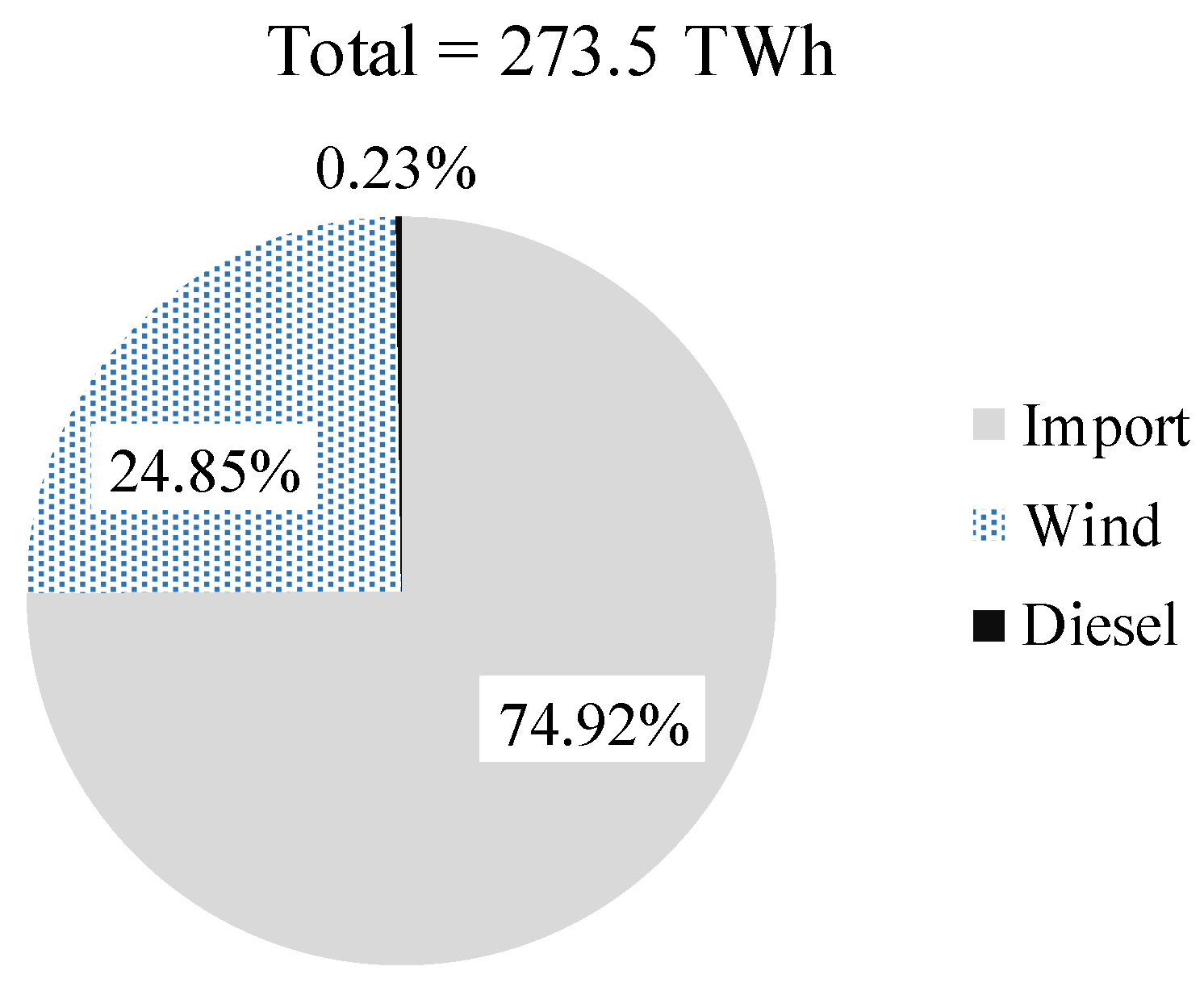
Figure 2 illustrates the City of Summerside energy supply mix between August 2016 to August 2018. Approximately 75% of the energy is supplied by importing power from NB Power inter-tie 69 kV line. Approximately 25% is supplied by the Summerside Electric wind farm, with only 0.23% of the energy supplied by diesel generation. Thus, throughout this paper, diesel generation is neglected, assuming that the energy is supplied by NB Power and the local wind farm.

3. Wind Power Prediction

Figure 3 demonstrates the hourly wind production and the power duration curve of the Summerside wind farm in 2017, revealing the high variability of the wind power output. In this figure, the gray line represents the hourly wind generation, and the black line demonstrates the total hours the power output is within a certain range. The objective is to predict wind power output for the next hour, 20 min in advance. Thus, the prediction procedure shown in Figure 4 is adopted, consisting of multiple steps. Each step is briefly described next, and the wind prediction results are provided at the end of this section.

3.1. Experimental Data

The experimental data used here for wind prediction are provided by Summerside Electric and Environment and Climate Change Canada and include the City of Summerside Electric and meteorological measurements. The data consist of three separate datasets: (i) dataset 1 has 17,568 data points of seven features corresponding to two years of hourly averaged data of Summerside Electric supervisory control and data acquisition (SCADA) system, measured from August 2016 to August 2018; (ii) dataset 2 has 52,560 data points of 98 features corresponding to one year of 10-minute averaged data of Summerside Electric wind turbines, measured from August 2017 to August 2018; and (iii) dataset 3 has 17,568 data points of 18 features corresponding to two years of hourly averaged meteorological data of the City of Summerside, measured from August 2016 to August 2018. Dataset 1 includes features such as power outputs of four wind turbines and wind speed. Dataset 2 includes features such as electrical data and turbines temperature. Dataset 3 includes features such as dew point temperature, air pressure, and relative humidity. A summary of the datasets is provided in Table 1.

3.2. Data Processing

The aforementioned datasets are processed prior to feature selection and predictor training phases. Data processing consists of two major steps: (i) data imputation, i.e., replacing missing data with substitute values; and (ii) stationarity test and treatment, i.e., eliminating trend and seasonality. In this case, less than 1% of all features of interest are missing values, which are simply replaced by their previous data point due to their insignificant portion of entire data. Thus, the rest of this subsection discusses treating time series non-stationarity, including trending and seasonality. Seasonality is the presence of cyclic patterns at specific regular intervals, such as daily, monthly, etc.; note that the interval is not necessary every season, i.e., a 3-month period.
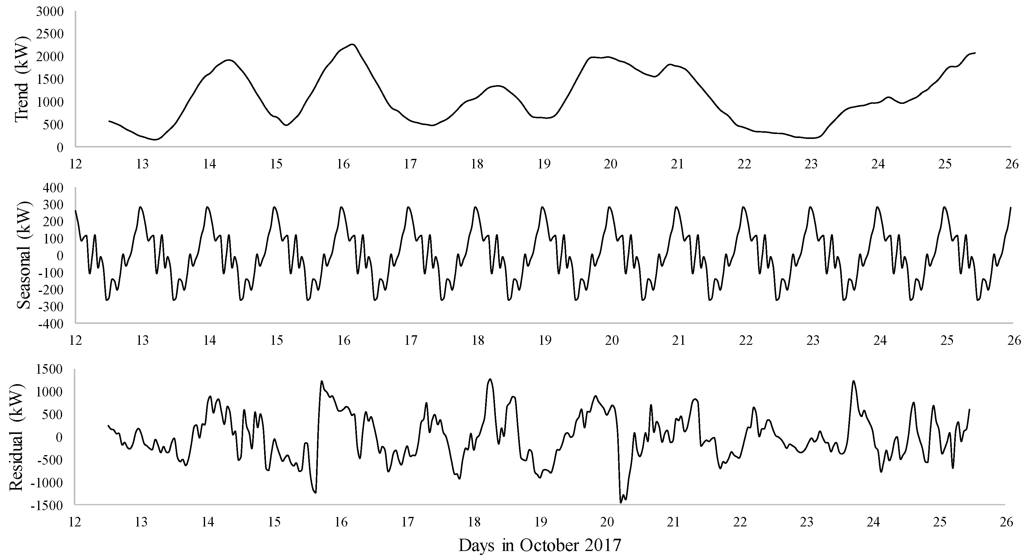
A time series is defined stationary if its generating process is time invariant [38]. Thus, statistical properties such as mean and variance of a stationary time series remain constant over time. It is known that non-stationarity adversely affects the accuracy of time series prediction, thus should be appropriately treated prior to forecasting [39]. To demonstrate this process and without loss of generality, a snippet of data is used as shown in Figure 5; the sample pertains to generation output of one turbine during a two-week period in October 2017. The outputs of other turbines are similar. As seen in Figure 5, visual observation cannot detect any pattern in data or in its mean and variance, mainly due to highly stochastic nature of wind output. To further evaluate the stationarity, two techniques are discussed next, namely augmented Dickey–Fuller (ADF) test and signal decomposition.
Statistical stationarity tests investigate time series mean non-stationarity, i.e., whether the series tend to move away from any initial point as time goes on [40]. Consider time series y t as follows:
Δ y t = T t + z t , T t = α + β t , z t = ϕ z t 1 + ϵ t , ϵ t N ( 0 , σ 2 ) ,
where α , β , and ϕ are constant parameters. Thus, time series y t is called trend stationary if ϕ 1 and is called difference stationary if ϕ = 1 . It is trivial to prove that difference stationary series can become stationary by differencing. Thus, the ADF test takes the null hypothesis that y t is trend stationary, i.e., the series has a unit root. Hence, the null hypothesis is rejected for p 0.05 . More details regarding AFD test implementation can be found in [38,39]. The ADF test on the sample data illustrated in Figure 5 returned a p-value of 4.9 × 10 5 , thus rejecting the null hypothesis. The p-value is even smaller for the entire time period, closer to 10 6 . It is concluded that no first differencing is needed in this case.
To further evaluate the data trend and seasonal pattern, it is decomposed into three components: (i) trend t r t ; (ii) seasonal s t ; and (iii) residual r t , as follows:
y t = t r t + s t + r t .
Note that Equation (2) presents an additive model for y t . The three additive components are basically calculated through moving averages; more details can be found in [41]. Figure 6 illustrates the three components of the original time series in Figure 5. As seen in Figure 6, there is a daily seasonal pattern, in the range of 600 kW peak-to-peak. Such a daily seasonality can be treated by 24th differencing, i.e., subtracting each data point by its 24th prior point.

3.3. Feature Selection

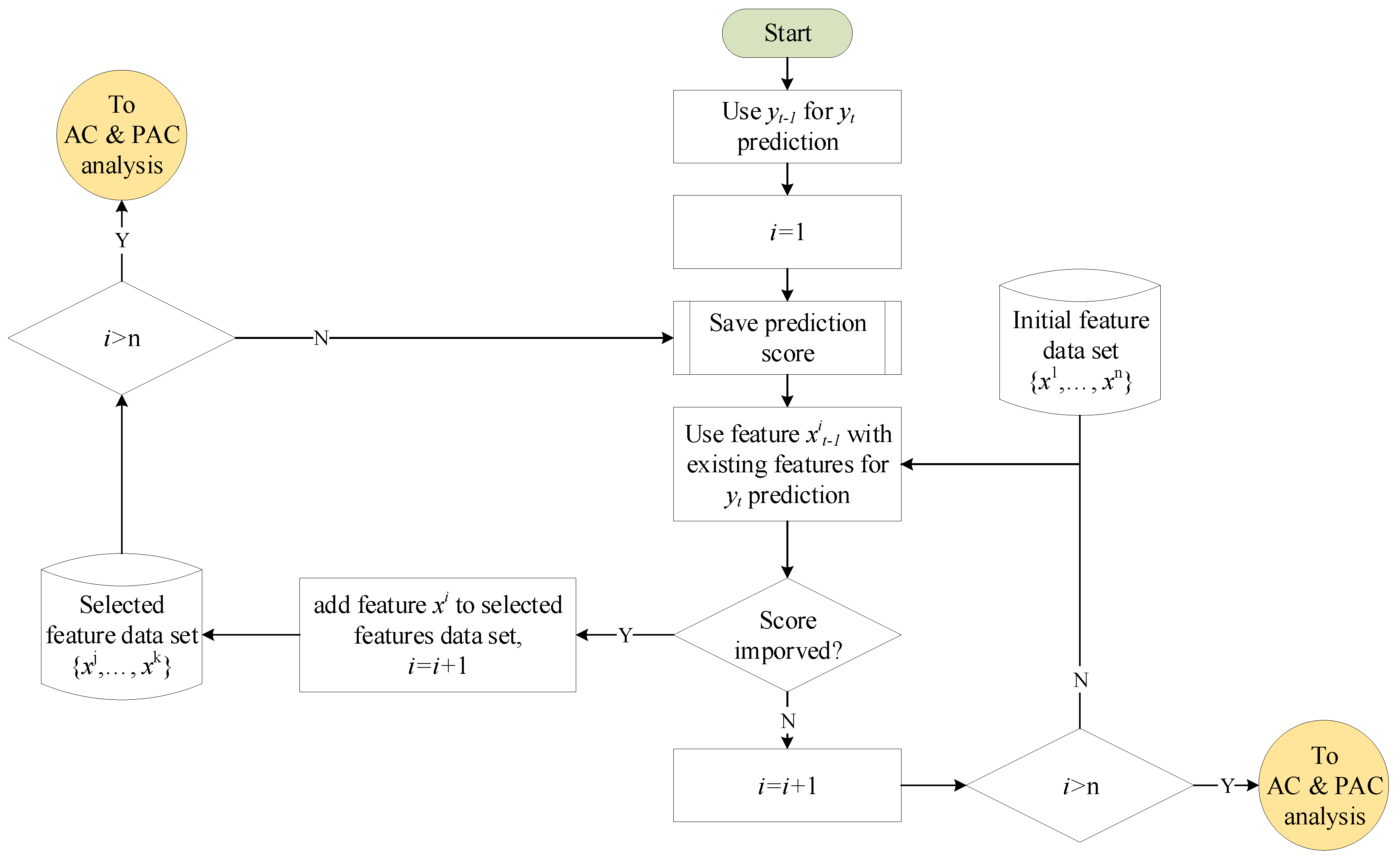
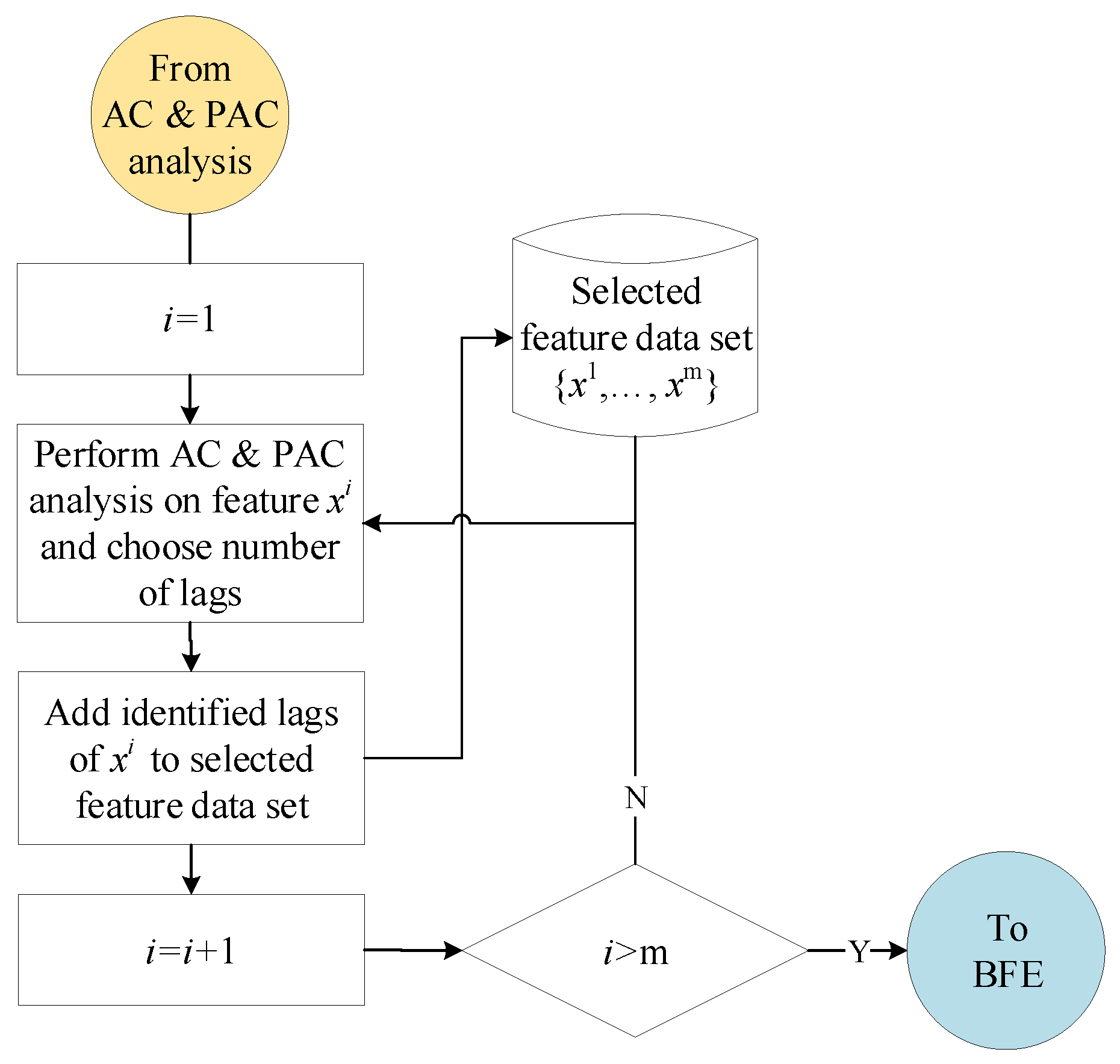
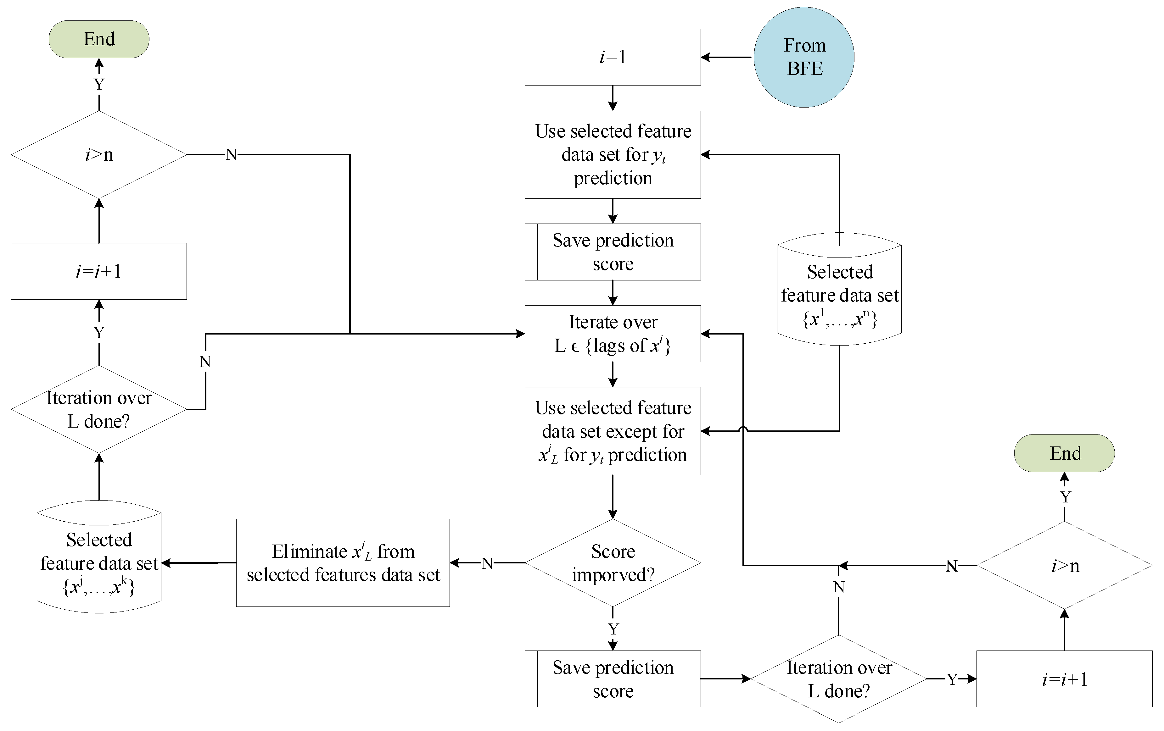
The processed datasets are analyzed to identify the predictive features. The presented feature selection in this case consists of three major steps: (i) forward feature selection (FFS); (ii) autocorrelation (AC) and partial autocorrelation (PAC) analysis; and (iii) backward feature elimination (BFE). The first step aims to identify predictive features using only first lag for each feature. The second step analyzes the predictive lags for each feature. Finally, the third step re-analyzes the included lags in an attempt to decrease the feature set dimension. Figure 7, Figure 8 and Figure 9 demonstrate the three steps of the process.
For brevity, FFS and BFE processes are not described as they can be properly inferred from Figure 7 and Figure 9. AC function calculates correlation coefficients of two values of the same time series at time t and its lagged observation t k . To calculate the AC coefficients, first, the autocovariance function at lag k is defined as follows:
γ k = 1 T t = k + 1 T y t y ¯ y t k y ¯ ,
where y ¯ is the time series mean. Thus, the AC function at lag k is defined as follows:
A C k = γ k γ 0 .
Note that γ 0 is the sample variance. PAC function also measures the correlation between y t and its lagged observations, but removes the influence of the observations in between two data points, as follows [12]:
P A C k = Corr y t P y t | y t k + 1 , , y t 1 , y t k P y t | y t k + 1 , , y t 1 ,
where P A | B is the best linear projection of A on B. Although both AC and PAC functions measures linear correlation, they can still be used for feature selection of nonlinear prediction methods, such as neural network techniques, as discussed in [42]. Thus, PAC function is used here for feature lag selection. As an example, Figure 10 depicts the PAC results for one of the Summerside Electric wind turbines, considering 48 lags equivalent to the past two days. As seen in this figure, the PAC between y t and its previous three lags onward is negligible, indicating low predictive value of these lags.

3.4. Results

The prediction model used in this case cannot be revealed due to commercial confidentiality. The predictor engine is tuned using the grid-search method [43]. Note that the main contribution of this section is to leverage a relatively large island grid’s actual data to reveal the potential of state-of-the-art RES prediction techniques. In addition, general procedures for enhancing RES prediction accuracy have been discussed so far using the actual data. Finally, the results discussed in this subsection are necessary for the data-driven BESS sizing discussed in Section 4. Thus, the results of Summerside hourly load prediction are also included.
Currently, SEETSS schedules the import power for the next hour 20 min in advance by subtracting the difference between load and wind predictions. SEETSS current predictions are provided by a third-party commercial company, whose prediction algorithm is not known. To evaluate the trained predictors and compare their performance with SEETSS existing ones, a 30-day period in Winter 2018 is used as the test set. Please note that, while there may be slight variations in the wind output profile depending on the season of the year, i.e., winter or summer, the results presented here are applicable to any period; the proposed techniques do not depend on the choice of the test set, and the 30-day period in winter is represented without the loss of generality. In case more than two years of data are available, this issue can be further investigated and verified.
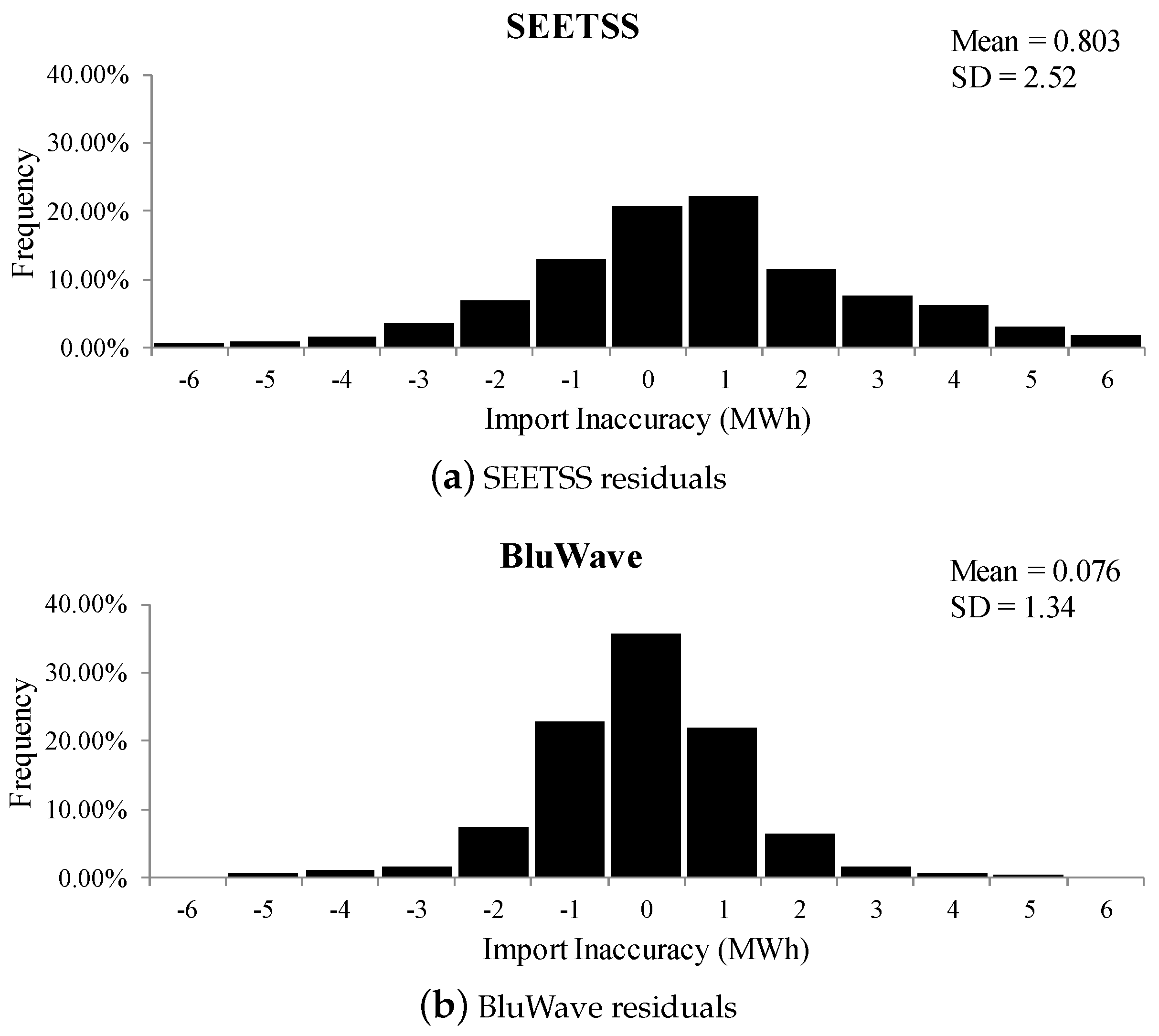
The error criterion in this case is mean absolute error (MAE), as inaccuracy in scheduled power directly maps to inaccuracy in absolute errors of wind and load prediction. Table 2 provides MAE of the load and wind predictions and the scheduled import energy. Note that the BluWave-ai and SEETSS predictors are referred to as BluWave and Summerside in the table, respectively. Histograms of SEETSS and BluWave import schedule residuals are illustrated in Figure 11.
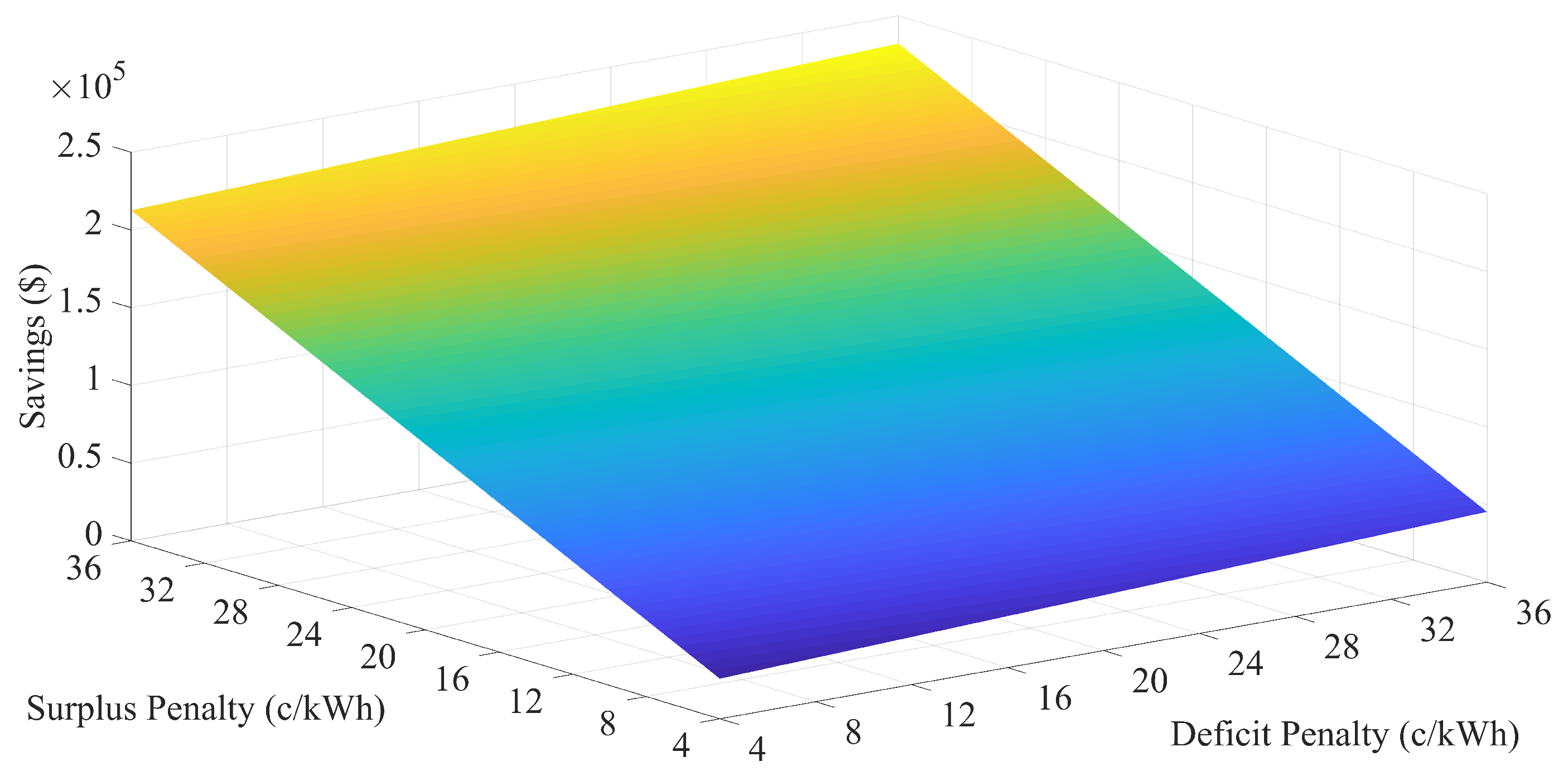
The results presented in Table 2 reveal a significant 48% reduction in import power inaccuracy using BluWave predictors. Figure 12 demonstrates savings as a result of the accuracy improvement under various energy surplus and deficit penalties, calculated as follows; note that the superscripts STS and BW stands for SEETSS and BluWave respectively:
Saving ( $ ) = i = 1 720 [ α i STS × Δ P i STS × ρ sur ( 1 α i STS ) × Δ P i STS × ρ def α i BW × Δ P i BW × ρ sur + ( 1 α i STS ) × Δ P i BW × ρ def ] ,  
where α i is a binary variable indicating surplus of energy, Δ P i is the import inaccuracy in MWh, and ρ sur and ρ def are energy surplus and deficit penalties in $/MWh accordingly.
As seen in Figure 12, a higher portion of savings occurs due to reduction in energy surplus as compared to energy deficit, indicated by the higher slope of the y-axis. This is expected as the SEETSS predictor is skewed toward positive residuals as seen in Figure 11. In other words, the BluWave predictor yields more accurate energy import schedules both by decreasing the mean and standard deviations of SEETSS import inaccuracy. Thus, the slope of the x-axis is $610 for each c/kWh of the deficit penalty, and the slope of the y-axis is $5840 for each c/kWh of the surplus penalty. For the case of Summerside Electric, the exact surplus and deficit penalties cannot be revealed due to contractual confidentiality between BluWave-ai, Summerside Electric, and NB Power; however, the penalties are toward the lower end of the spectrum, in the range of ∼12 c/kWh. In the next section, residuals shown in Figure 11 are used for a data-driven energy storage sizing.

4. Data-Driven BESS Sizing

In this section, a data-driven BESS sizing method is proposed to minimize the cost of import scheduling inaccuracy, taking the BESS investment cost into account. For the proposed technique, the impact of long-term load growth is neglected, and the interest and inflation rates are assumed zero.

4.1. Battery Characteristics

A lithium-ion battery (LIB) is considered for the purpose of this research. Lithium-ion batteries have been widely used for large-scale grid applications and can discharge their full energy as fast as in 20 min [44]. To quantify the charge and discharge capability, C-rate is defined as the ratio of BESS nominal power to energy capacity. Grid-scale LIB investment cost depends on both its energy capacity and C-rate. Thus, various investment costs have been reported in the literature. For the case of this research, three C-rates of 1, 2, and 3 are considered and the BESS investment cost reported in Table 3 is chosen based on the National Renewable Energy Laboratory (NREL) report on LIB cost in 2018, as well as experts’ analysis on prospective improvements in LIB costs [45,46].
Battery aging model has been the subject of research for a few decades, and numerous models have been proposed in the literature [47,48,49]. Generally, battery aging can be decomposed into calendric and cyclic aging effects [44]. These components determine the battery state of health (SOH), i.e., the degradation in its nominal capacity. For the case of this study, it is assumed that the BESS has a nominal 10,000 cycles and a calendric age of 15 years, and cannot be used beyond an SOH of 80% [50]. Thus, the impact of calendric and cyclic aging on BESS SOH is expressed by Equation (7). Note that more complex aging models can be adopted, as the proposed sizing method is quite flexible and effective in taking complexities and nonlinearities into account:
SOH = 1 0.2 | P B | Δ τ E B × 10,000 0.2 × Δ τ 15 × 365 × 24 .
In Equation (7), Δ τ is the time-step length, P b is the average battery charged or discharged power, and E b is the battery nominal energy capacity. The battery should be replaced when SOH reaches 80%.

4.2. Methodology

Table 4 summarizes the notation used in this subsection. The method proposed herein has four steps and adopts a Monte Carlo simulation technique [51], as follows:
  • Populate a set of import inaccuracies vector, S , based on the results presented in Figure 11.
  • Populate a set of BESS energy capacity, E . For each element in E , populate a set of C-rates, C .
  • For each element in E and its corresponding elements in C , calculate the charged and discharged energies for each element in S . Calculate the savings by reducing investment cost from energy savings. Thus, for each simulation scenario b , c , there exist s simulation scenarios b , c , s .
  • Calculate the final savings for each element in E and its corresponding elements in C by averaging the savings calculated for the elements in S .
For the case of this study, S has 1000 elements. Each element is a vector of 131,400 randomly generated numbers, corresponding to 15 years of hourly interval time-steps set, T . Random numbers are drawn from N ( 0.076 , 1.34 ) based on the results presented in Figure 11. E has 59 elements corresponding to nominal energy capacity range of 0.5–15 MWh with steps of 0.25 MWh. C has three elements, 1, 2, and 3. Thus, a total of 177 simulation scenarios b , c are carried out 1000 times each iterating over S , making a total of 177,000 simulations.
To calculate the charged and discharged energy during each time-step, first, the equality and inequality constraints should be modeled to consider for BESS operational limits, energy evolution, and aging, as follows:
P b , c = E b × C c = E b × C c b E c C ,
E s , i b , c = E s , i 1 b , c + E c h s , i b , c η E d i s s , i b , c η Δ τ b E c C s S i T ,
SOH s , i b , c = SOH s , i 1 b , c 0.2 E c h s , i b , c + E d i s s , i b , c Δ τ E b × 1000 0.2 × Δ τ 131,400 b E c C s S i T ,
0.1 × E B E s , i b , c 0.9 × SOH s , i b , c × E B b E c C s S i T .
Equation (8) calculates BESS nominal power based on nominal energy capacity and C-rate. Equations (9) and (10) model the BESS energy and SOH evolution, respectively. Finally, Equation (11) constrains the BESS energy between 10% of its nominal capacity and 90% of its nominal capacity multiplied by SOH.
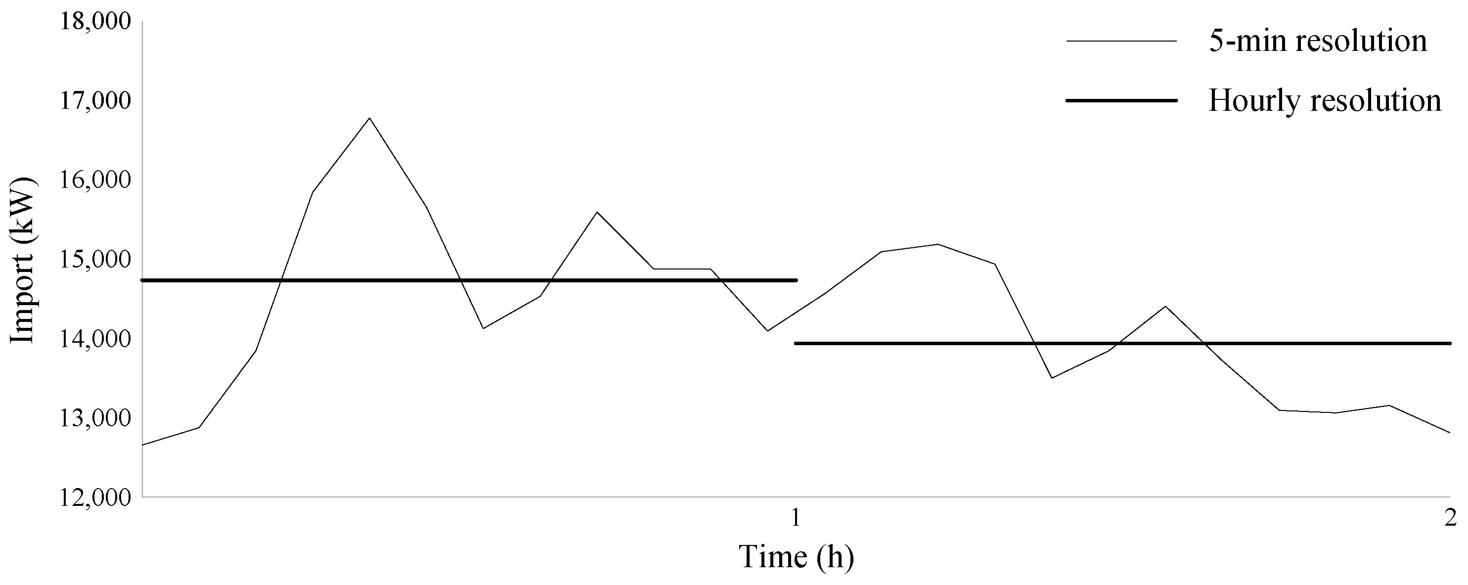
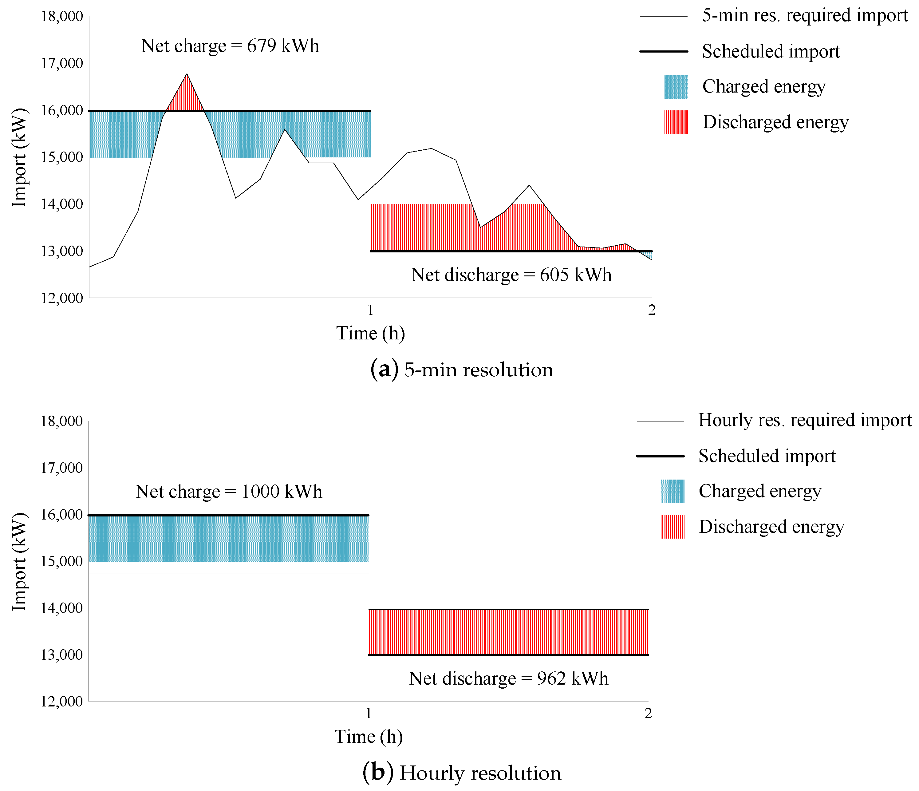
To calculate the BESS charged and discharged energy during each time-step, one should consider not only the energy import inaccuracy and BESS state of charge and capacity, but also BESS nominal power capacity. To account for the latter, researchers often divide the required energy by time-interval length to arrive at an average required power [29,30,31,32,33,34,35,36]. However, such an approach does not take into account the power variations within the interval, which may go beyond the nominal power of the BESS, resulting in a trade-off between accuracy and time-interval resolution. This is demonstrated in Figure 13, where a 2-h sample of Summerside Electric import is shown in 5-min and hourly resolutions. To demonstrate the impact of time resolution on charged and discharged energy calculation, assume that the BESS nominal power capacity is 1 MW. Thus, Figure 14 shows the difference between calculated charged and discharged energy for the same 2-h sample period but with different time resolutions. As seen in this figure, low resolution may yield over-estimation of charged and discharged energy, 321 kWh of charged and 357 kWh of discharged energy in this case.
A novel data-driven approach is proposed here to address the negative impact of low resolution on over-estimation of charged and discharged energy. Thus, four months of 5-min averaged data pertaining to Summerside Electric actual required import between November 2018 to February 2019 is utilized to design the proposed solution. The first part of the solution is to estimate the energy content above and below the averaged required power during each hourly interval, as follows:
  • Calculate the hourly averaged power.
  • Populate a set of power threshholds. In this case, the power threshold ranges from 0–1000 kW with steps of 50 kW.
  • Calculate the energy above and below the average required power for each power threshold.
  • Calculate the average of calculated energies for each power threshold.
  • Fit the appropriate trendline to the calculated average energy of power thresholds [52]. In this case, an exponential trendline is chosen based on the observed data. The trendline expression can be used to estimate the energy above and below the hourly average required power for a certain power threshold.
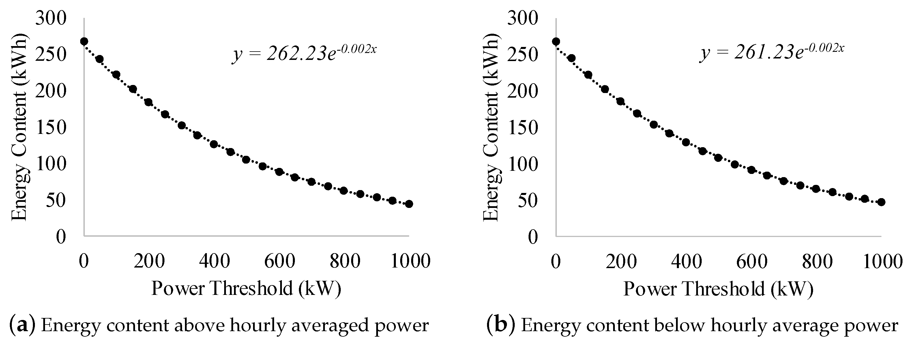
Figure 15 demonstrates the result of the above-mentioned procedure. Here is an example to clarify the results presented in this figure. Suppose the average hourly required power for time-step i is 10 MW, thus the required energy import is 10 MWh. Out of this 10 MWh, around 260 kWh pertains to intra-interval duration when imported power is higher than 10 MW, and less than 50 kWh pertains to duration when the intra-interval import power is higher than 11 MW. As expected, the energy content above and below the hourly average required power is symmetrical; hence, the two exponential equations presented in Figure 15 are averaged to estimate the energy content both above and below the averaged hourly required power, as follows:
Estimated Energy ( kWh ) = e f P ( kW ) = 261.73 × e 0.002 P .
The next step is to use e f ( P ) to calculate the charged and discharged energy during each time-step, taking Equations (8)–(11) into consideration. Here is the procedure for time-steps with energy surplus:
  • α i = 1, i.e., there is surplus of energy Δ e i .
  • If Equation (13) is true, i.e., the average surplus power within the time interval does not exceed the battery power rating, go to step 3, otherwise go to step 6:
    Δ e i Δ τ P b , c .
  • Estimate BESS charged energy using Equation (14):
    E c h s , i b , c = Δ e i e f P b , c Δ e i Δ τ .
  • If Equation (15) is true, i.e., the battery energy content at the end of the time interval does not exceed the maximum acceptable energy capacity, end the process and go to the next time step, otherwise go to step 5:
    E s , i 1 b , c + E c h s , i b , c × η 0.9 × SOH s , i 1 b , c × E b .
  • Estimate the BESS charged energy using Equation (16); end the process and go to the next time step:
    E c h s , i b , c = 0 . 9 × SOH s , i 1 b , c × E b E s , i 1 b , c η .
  • Estimate BESS charged energy using Equation (17):
    E c h s , i b , c = P b , c × Δ τ e f Δ e i Δ τ P b , c .
  • If Equation (15) is true, end the process and go to the next time step, otherwise go to step 8.
  • Estimate the charged energy using Equation (16); end the process and go to the next time step.
The procedure for time-steps with deficit of energy is similar to above, as follows:
  • α i = 0, i.e., there is deficit of energy Δ e i .
  • If Equation (13) is true, go to step 3, otherwise go to step 6.
  • Estimate BESS charged energy using Equation (18):
    E d i s s , i b , c = Δ e i e f P b , c Δ e i Δ τ .
  • If Equation (19) is true, i.e., the battery energy content at the end of the time interval is not below the minimum acceptable energy capacity, end the process and go to the next time step, otherwise go to step 5:
    0.1 × E b E s , i 1 b , c E d i s s , i b , c η .
  • Estimate the BESS charged energy using Equation (20); end the process and go to the next time step:
    E d i s s , i b , c = E d i s s , i 1 b , c 0.1 × E b × η .
  • Estimate BESS charged energy using Equation (21):
    E d i s s , i b , c = P b , c × Δ τ e f Δ e i Δ τ P b , c .
  • If Equation (19) is true, end the process and go to the next time step, otherwise go to step 8.
  • Estimate the charged energy using Equation (20); end the process and go to the next time step.
The proposed methodology in this subsection is presented in Figure 16. Note that, in this figure, indices b, c, and s are omitted for the sake brevity. In addition, as Δ τ = 1 , it is also omitted. As seen in Figure 16, the BESS charged and discharged energy is calculated for each time-step until the BESS reaches an SOH of 80%. Once the charged and discharged energy are calculated for each scenario s, the overall scenario savings can be calculated as follows:
Save s b , c = i = 1 131400 [ α i × E c h s , i b , c × ρ sur + ( 1 α i ) × E d i s s , i b , c × ρ def ] Investment b , c ,
where Save s b , c is the overall scenario cost, Investment b , c is the BESS investment cost calculated based on Table 3, and ρ s u r and ρ d e f are energy surplus and deficit penalties, respectively. Thus, the levelized cost of BESS investment can be calculated using Equation (23). Note that a negative savings indicates that BESS investment is not economically justifiable:
Save Levelized b , c = s = 1 1000 Save s b , c / L s b , c 1000 .

5. Economics of the Wind-BESS System

This section presents the results obtained from conducting the data-driven method presented in Section 4. The results included here only pertain to the C-rate of 1, omitting the results for C-rates of 2 and 3 as these were found to be always economically inferior to the C-rate of 1. The results are obtained over a range of surplus and deficit penalties, from 4 to 36 c/kWh with steps of 4.

5.1. Optimal BESS Capacity

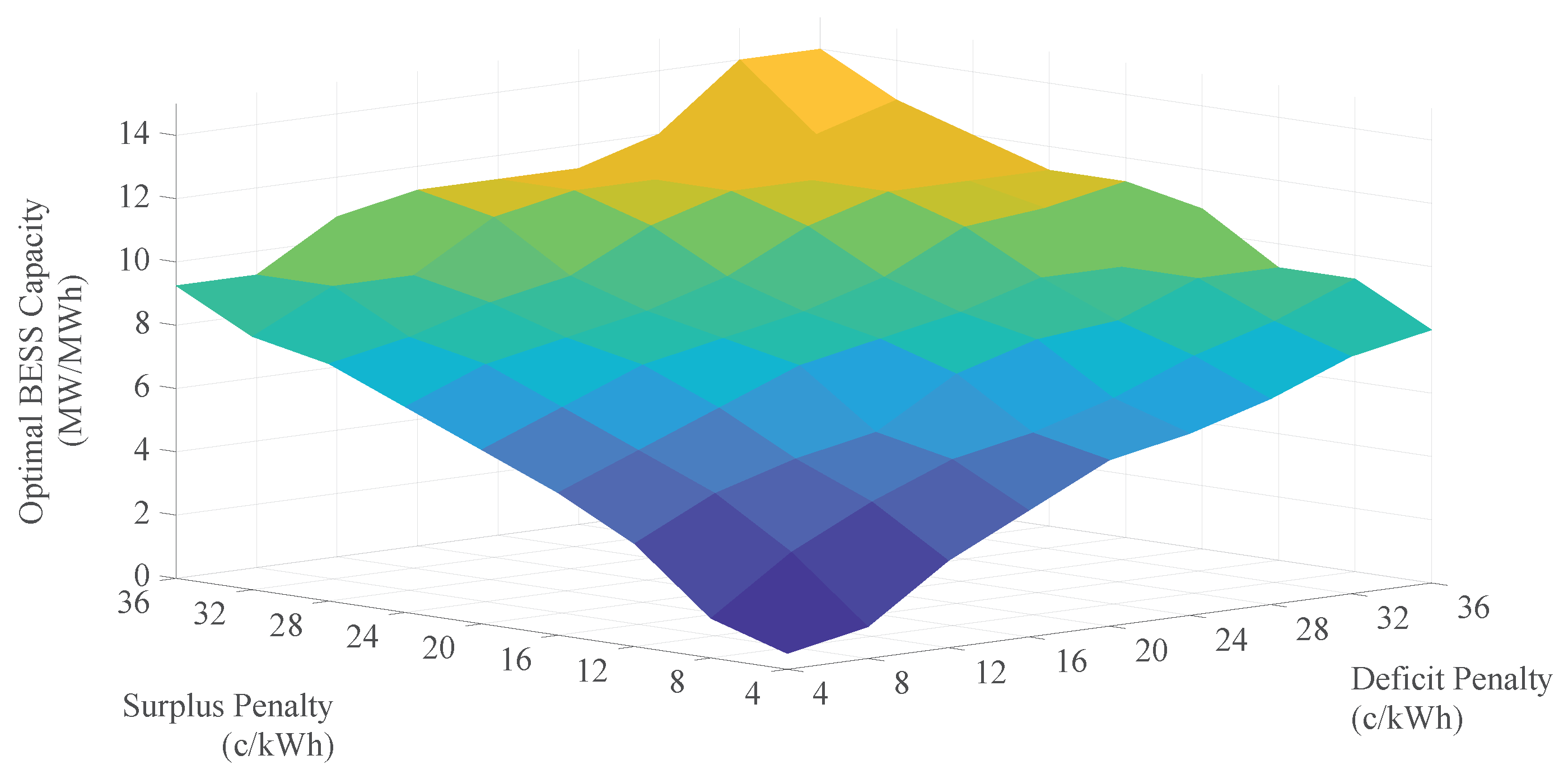
Figure 17 presents the BESS capacity that yields the highest levelized savings for each price range. The same results are presented numerically in Table 5. As expected, the optimal BESS capacity is higher for higher surplus and deficit penalties.

5.2. Highest Achievable Savings

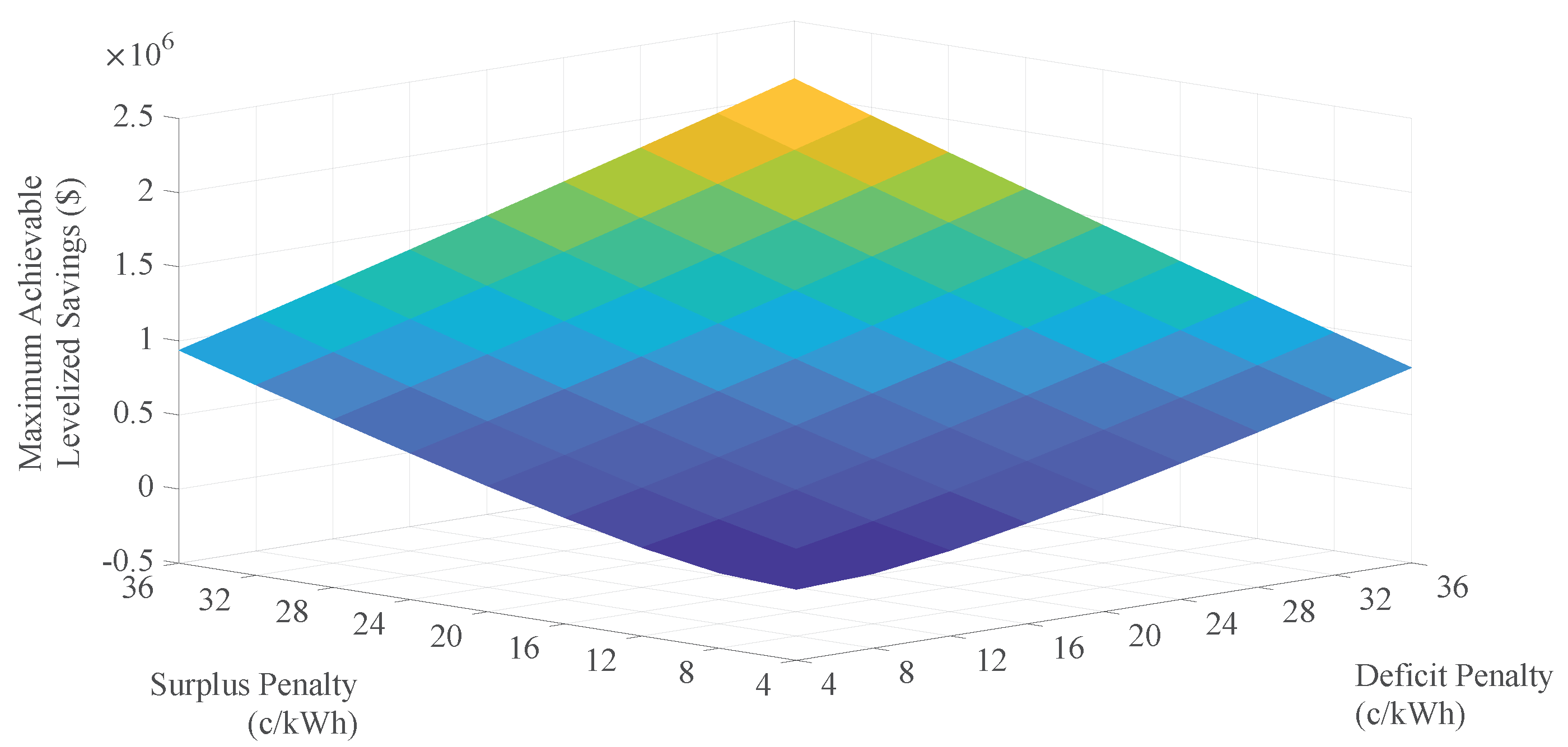
Figure 18 presents the highest achievable levelized savings for each price range. The same results are presented numerically in Table 6. As expected, the highest achievable savings increases as the surplus and deficit penalties increase.

5.3. BESS Lifetime

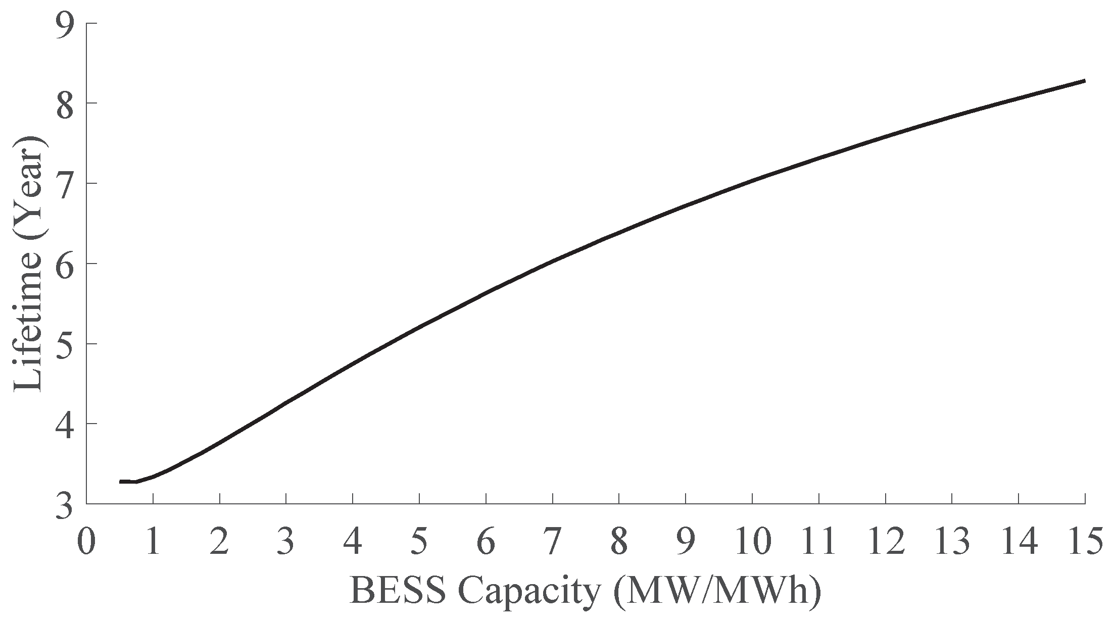
Figure 19 presents the amount of time it takes to reach an SOH of 80% for various BESS capacities. As BESS capacity increases, its lifetime also increases because of slower cycling aging.

5.4. Interpretation and Analysis

Results presented in Figure 17, Figure 18 and Figure 19 and Table 5 and Table 6 enable the optimal choice of BESS size over the 15-year course of the project. Without loss of generality, surplus and deficit penalties of 8 c/kWh and 16 c/kWh are used as an example here; the analysis for the rest of penalty prices is similar. Referring to Table 5, it can be concluded that a 5.25 MWh BESS yields the highest achievable levelized savings of $308,000. Referring to Figure 19, such BESS takes approximately 5 years to reach an SOH of 80%, i.e., it should be replaced after five years. To fulfill the project lifetime of 15 years, it can be concluded that a 15.75 MWh/5.25 MW BESS would yield the highest achievable levelized cost for the entire 15-year period. Thus, the general procedure to obtain the optimal BESS energy and power capacity for any project lifetime is as follows:
  • From Table 5, find the optimal power, P opt .
  • From Figure 19, find the BESS lifetime, B L .
  • Set the project lifetime, P L .
  • Using Equation (24), find the optimal energy capacity, E opt :
    E opt = P opt P L B L .
Using the above-mentioned process, Table 7 provides the optimal BESS energy and power capacity for the 15-year project. Considering penalties of ∼12 c/kWh, the optimal BESS sizing for the case of Summerside Electric is 5.25 MW and 15 MWh of BESS power and energy capacity respectively, which would yield an annual levelized net savings of ∼$322,000.
Considering the results presented herein, it can be concluded that, for almost all ranges of surplus and deficit penalties, BESS investment yields significant savings. Note that these savings would be on top of savings due to more accurate predictors, previously presented in Figure 12.

6. Conclusions

Two years of data from Summerside Electric are leveraged to reveal the potential to mitigate the negative impact of RES variability on energy scheduling of renewable-penetrated grids. Thus, the procedure to process data and prepare it for RES prediction is outlined. It is demonstrated that state-of-the-art time series predictors can bring significant operational savings. The results obtained from time series prediction is utilized to propose a novel data-driven BESS sizing technique for energy scheduling applications in renewable-penetrated grids and microgrids. The data-driven approach mitigates the trade-off between data resolution and accuracy, and provides a robust methodology to consider for both BESS energy and power nominal rating. It is shown that a properly sized BESS can bring significant savings for a wide range of energy surplus and deficit penalties, even in the presence of accurate RES and load predictors. Please note that any of the proposed techniques, including the data-driven BESS sizing, are applicable to other grids with similar operation paradigm, as long as the necessary data is provided and processed accordingly. Future work can extend the proposed data-driven BESS sizing approach to take other grid applications and ancillary services into account.

Funding

This research and the submission fee is funded by BluWave-ai.

Acknowledgments

The author would like to thank Greg Gaudet and Gerald Giroux from Summerside Electric, and Lutz Tischendorf from BluWave-ai for providing the data necessary for this research.

Conflicts of Interest

The author declares no conflict of interest. The funders had no role in the design of the study; in the collection, analyses, or interpretation of data; in the writing of the manuscript, or in the decision to publish the results.

Abbreviations

The following abbreviations are used in this manuscript:
ACAutocorrelation
ADFAugmented Dickey–Fuller
AIArtificial Intelligence
ARIMAAutoregressive Integrated Moving Average
BESSBattery Energy Storage Systems
BFEBackward Feature Elimination
ESSEnergy Storage Systems
LIBLithium-Ion Battery
MAEMean Absolute Error
MOUMemorandum of Understanding
NRELNational Renewable Energy Laboratory
NWPNumerical Weather Prediction
PACPartial Autocorrelation
PEIPrince Edward Island
RESRenewable Energy Resources
SCADASupervisory Control and Data Acquisition
SEETSSSummerside Electric Energy Transmission Scheduling System
SOHState of Health
SVMSupport Vector Machine

References

  1. Nanaki, E.A.; Xydis, G.A. Deployment of Renewable Energy Systems: Barriers, Challenges, and Opportunities. Adv. Renew. Energies Power Technol. 2018, 2, 207–229. [Google Scholar]
  2. Eftekharnejad, S.; Vittal, V.; Heydt, G.T.; Keel, B.; Loehr, J. Impact of increased penetration of photovoltaic generation on power systems. IEEE Trans. Power Syst. 2013, 28, 893–901. [Google Scholar] [CrossRef]
  3. Ulbig, A.; Borsche, T.S.; Andersson, G. Impact of Low Rotational Inertia on Power System Stability and Operation. IFAC Proc. Vol. 2014, 47, 7290–7297. [Google Scholar] [CrossRef] [Green Version]
  4. Wang, J.; Botterud, A.; Bessa, R.; Keko, H.; Carvalho, L.; Issicaba, D.; Sumaili, J.; Miranda, V. Wind Power Forecasting Uncertainty and Unit Commitment. Appl. Energy 2011, 88, 4014–4023. [Google Scholar] [CrossRef]
  5. Farrokhabadi, M.; Konig, S.; Canizares, C.A.; Bhattacharya, K.; Leibfried, T. Battery Energy Storage System Models for Microgrid Stability Analysis and Dynamic Simulation. IEEE Trans. Power Syst. 2018, 33, 2301–2312. [Google Scholar] [CrossRef]
  6. Hong, T.; Pinson, P.; Fan, S. Global Energy Forecasting Competition 2012. Int. J. Forecast. 2014, 30, 357–363. [Google Scholar] [CrossRef]
  7. Marugan, A.P.; Marquez, F.P.G.; Perez, J.M.P.; Ruiz-Hernandez, D. A Survey of Artificial Neural Network in Wind Energy Systems. Appl. Energy 2018, 228, 1822–1836. [Google Scholar] [CrossRef]
  8. Ordinao, J.A.G.; Waczowicz, S.; Hegenmeyer, V.; Mikut, R. Energy Forecasting Tools and Services. WIREs Data Min. Knowl. Discov. 2018, 8, 1–20. [Google Scholar]
  9. Wong, S.; Gaudet, G.; Proulx, L. Capturing Wind with Thermal Energy Storage-Summerside’s Smart Grid Approach. IEEE Power Energy Technol. Syst. J. 2017, 4, 115–124. [Google Scholar] [CrossRef]
  10. Mi, Z.; Jia, Y.; Wang, J.; Zheng, X. Optimal Scheduling Strategies of Distributed Energy Storage Aggregator in Energy and Reserve Markets Considering Wind Power Uncertainties. Energies 2018, 11, 1242. [Google Scholar] [CrossRef]
  11. Stein, K.; Tun, M.; Musser, K.; Rocheleau, R. Evaluation of a 1 MW, 250 kW-hr Battery Energy Storage System for Grid Services for the Island of Hawaii. Energies 2018, 11, 3367. [Google Scholar] [CrossRef]
  12. Feng, C.; Cui, M.; Hodge, B.; Zhang, J. A data-driven multi-model methodology with deep feature selection for short-term wind forecasting. Appl. Energy 2017, 190, 1245–1257. [Google Scholar] [CrossRef] [Green Version]
  13. Richardson, L.F. Weather Prediction by Numerical Process; Cambridge University Press: New York, NY, USA, 2007. [Google Scholar]
  14. Ma, L.; Luan, S.; Jiang, C.; Liu, H.; Zhang, Y. A Review on the Forecasting of Wind Speed and Generated Power. Renew. Sustain. Energy Rev. 2009, 3, 915–920. [Google Scholar]
  15. Al-Yahyai, S.; Charabi, Y.; Gastli, A. Review of the Use of Numerical Weather Prediction (NWP) Models for Wind Energy Assessment. Renew. Sustain. Energy Rev. 2010, 14, 3192–3198. [Google Scholar] [CrossRef]
  16. Cadenas, E.; Rivera, W.; Campos-Amezcua, R.; Heard, C. Wind Speed Prediction Using a Univariate ARIMA Model and a Multivariate NARX Model. Energies 2016, 9, 109. [Google Scholar] [CrossRef]
  17. Poncela, M.; Poncela, P.; Peran, J. Automatic Tuning of Kalman Filters by Maximum Likelihood Methods for Wind Energy Forecasting. Appl. Energy 2013, 108, 349–362. [Google Scholar] [CrossRef]
  18. Santamaria-Bonfil, G.; Reyes-Ballesteros, A.; Gershenson, C. Wind Speed Forecasting for Wind Farms: A Method Based on Support Vector Regression. Renew. Energy 2016, 56, 790–806. [Google Scholar] [CrossRef]
  19. Chang, G.; Lu, H.; Chang, Y.; Lee, Y. An Improved Neural Network-based Approach for Short-Term Wind Speed and Power Forecast. Renew. Energy 2017, 105, 301–311. [Google Scholar] [CrossRef]
  20. Doucoure, B.; Agbossou, K.; Cardenas, A. Time Series Prediction Using Artificial Wavelet Neural Network and Multi-Resolution Analysis: Application to Wind Speed Data. Renew. Energy 2016, 92, 202–211. [Google Scholar] [CrossRef]
  21. Chow, T.; Li, S.; Fang, Y. A Real-Time Learning Control Approach for Nonlinear Continuous-Time System Using Recurrent Neural Networks. IEEE Trans. Ind. Electr. 2000, 47, 478–486. [Google Scholar] [CrossRef]
  22. Sanchez, I. Adaptive Combination of Forecasts with Application to Wind Energy. Int. J. Forecast. 2008, 24, 679–693. [Google Scholar] [CrossRef]
  23. Delille, G.; Franois, B.; Malarange, G. Dynamic Frequency Control Support by Energy Storage to Reduce the Impact of Wind and Solar Generation on Isolated Power System’s Inertia. IEEE Trans. Sustain. Energy 2012, 3, 931–939. [Google Scholar] [CrossRef]
  24. Farrokhabadi, M.; Solanki, B.V.; Canizares, C.A.; Bhattacharya, K.; Koenig, S.; Sauter, P.S.; Leibfried, T.; Hohmann, S. Energy Storage in Microgrids: Compensating for Generation and Demand Fluctuations While Providing Ancillary Services. IEEE Power Energy Mag. 2017, 15, 81–91. [Google Scholar] [CrossRef]
  25. Lo, C.; Anderson, M.A. Economic Dispatch and Optimal Sizing of Battery Energy Storage Systems in Utility Load-Leveling Operations. IEEE Trans. Energy Convers. 1999, 14, 824–829. [Google Scholar] [CrossRef]
  26. Nottrott, A.; Klessl, J.; Washom, B. Energy Dispatch Schedule Optimization and Cost Benefit Analysis for Grid-Connected, Photovoltaic-Battery Storage Systems. Renew. Energy 2013, 55, 230–240. [Google Scholar] [CrossRef]
  27. Bathurst, G.; Strbac, G. Value of Combining Energy Storage and Wind in Short-Term Energy and Balancing Markets. Electr. Power Syst. Res. 2003, 67, 1–8. [Google Scholar] [CrossRef]
  28. Arefi, A.; Shahnia, F.; Ledwich, G. Electric Distribution Network Management and Control; Springer: Singapore, 2018. [Google Scholar]
  29. Hesse, H.C.; Martins, R.; Musilek, P.; Naumann, M.; Truong, C.N.; Jossen, A. Economic Optimization of Component Sizing for Residential Battery Storage Systems. Energies 2017, 10, 835. [Google Scholar] [CrossRef]
  30. Ying, Y.; Bremnera, S.; Menictasb, C.; Kaya, M. Battery Energy Storage System Size Determination in Renewable Energy Systems: A Review. Renew. Sustain. Energy Rev. 2018, 91, 109–125. [Google Scholar] [CrossRef]
  31. Wu, J.; Zhang, B.; Li, H.; Li, Z.; Chen, Y.; Miao, X. Statistical Distribution for Wind Power Forecast Error and its Application to Determine Optimal Size of Energy Storage System. Int. J. Electr. Power Energy Syst. 2014, 55, 100–107. [Google Scholar] [CrossRef]
  32. Tan, C.W.; Green, T.C.; Hernandez-Aramburo, C.A. A Stochastic Method for Battery Sizing with Uninterruptible Power and Demand Shift Capabilities in PV (photovoltaic) systems. Energy 2010, 35, 5082–5092. [Google Scholar] [CrossRef]
  33. Nguyen, T.A.; Crow, M.L.; Elmore, A.C. Optimal Sizing of a Vanadium Redox Battery System for Microgrid Systems. IEEE Trans. Sustain. Energy 2015, 6, 729–737. [Google Scholar] [CrossRef]
  34. Bahramirad, S.; Reder, W.; Khodaei, A. Reliability-Constrained Optimal Sizing of Energy Storage System in a Microgrid. IEEE Trans. Smart Grid 2012, 3, 2056–2062. [Google Scholar] [CrossRef]
  35. Fossati, J.P.; Galarza, A.; Martin-Villate, A.; Fontan, L. A Method for Optimal Sizing Energy Storage Systems for Microgrids. Renew. Energy 2015, 77, 539–549. [Google Scholar] [CrossRef]
  36. Saboori, H.; Hemmati, R.; Jirdehi, M.A. Reliability Improvement in Radial Electrical Distribution Network by Optimal Planning of Energy Storage Systems. Energy 2015, 93, 2299–2312. [Google Scholar] [CrossRef]
  37. Summerside, Prince Edward Island. Available online: https://en.wikipedia.org/wiki/Summerside,_Prince_Edward_Island (accessed on 9 February 2019).
  38. Brockwell, P.J.; Davis, R.A. Introduction to Time Series and Forecasting; Springer: Cham, Switzerland, 2016. [Google Scholar]
  39. Virili, F.; Freisleben, B. Nonstationarity and Data Preprocessing for Neural Network Predictions of an Economic Time Series. In Proceedings of the IEEE-INNS-ENNS International Joint Conference on Neural Networks, Como, Italy, 27 July 2000; pp. 129–134. [Google Scholar]
  40. Nelson, C.R.; Plosser, C.R. Trends and Random Walks in Macroeconmic Time Series: Some Evidence and Implications. J. Monet. Econ. 1982, 10, 139–162. [Google Scholar] [CrossRef]
  41. Makridakis, S.; Wheelwright, S.; Hyndman, R. Forecasting: Methods and Applications; Wiley: New York, NY, USA, 1997. [Google Scholar]
  42. Flores, J.H.F.; Engel, P.M.; Pinto, R.C. Autocorrelation and Partial Autocorrelation Functions to Improve Neural Networks Models on Univariate Time Series Forecasting. In Proceedings of the 2012 International Joint Conference on Neural Networks (IJCNN), Brisbane, QLD, Australia, 10–15 June 2012; pp. 1–8. [Google Scholar]
  43. Bao, Y.; Zhitao, L. A Fast Grid Search Method in Support Vector Regression Forecasting Time Series. In Proceedings of the International Conference on Intelligent Data Engineering and Automated Learning (IDEAL), Burgos, Spain, 20–23 September 2006; pp. 504–511. [Google Scholar]
  44. Martins, R.; Hesse, H.C.; Jungbauer, J.; Vorbuchner, T.; Musilek, P. Optimal Component Sizing for Peak Shaving in Battery Energy Storage System for Industrial Applications. Energies 2018, 11, 2048. [Google Scholar] [CrossRef]
  45. Fu, R.; Remo, T.; Margolis, R. 2018 U.S. Utility-Scale Photovoltaics-Plus-Energy Storage System Costs Benchmark; Technical Report TP-6A20-71714; National Renewable Energy Laboratory (NREL): Denver, CO, USA, 2018.
  46. Few, S.; Schmidt, O.; Offer, G.J.; Brandon, N.; Nelson, J.; Gambhir, A. Prospective Improvements in Cost and Cycle Life of Off-Grid Lithium-Ion Battery Packs: An Analysis Informed by Expert Elicitations. Energy Policy 2018, 114, 578–590. [Google Scholar] [CrossRef]
  47. Vetter, J.; Novak, P.; Wagner, M.R.; Veit, C.; Moller, K.C.; Besenhard, J.O.; Winter, M.; Wohlfahrt-Mehrens, M.; Vogler, C.; Hammouche, A. Ageing Mechanisms in Lithium-Ion Batteries. J. Power Sources 2005, 147, 269–328. [Google Scholar] [CrossRef]
  48. Battke, B.; Schmidt, T.S.; Grosspietsch, D.; Hoffmann, V.H. A Review and Probabilistic Model of Lifecycle Costs of Stationary Batteries in Multiple Applications. Renew. Sustain. Energy Rev. 2013, 25, 240–250. [Google Scholar] [CrossRef]
  49. Barre, A.; Deguilhem, B.; Grolleau, S.; Gerard, M.; Suard, F.; Riu, D. A Review on Lithium-Ion Battery Ageing Mechanisms and Estimations for Automotive Applications. J. Power Sources 2013, 241, 680–689. [Google Scholar] [CrossRef]
  50. Hesse, H.C.; Schimpe, M.; Kucevic, D.; Jossen, A. Lithium-Ion Battery Storage for the Grid—A Review of Stationary Battery Storage System Design Tailored for Applications in Modern Power Grids. Energies 2017, 10, 2107. [Google Scholar] [CrossRef]
  51. Rubinstein, R.Y.; Kroese, D.P. Simulation and the Monte Carlo Method; John Wiley & Sons: Hoboken, NJ, USA, 2016. [Google Scholar]
  52. Guest, P.G. Numerical Methods of Curve Fitting; Cambridge University Press: Cambridge, UK, 2013. [Google Scholar]
Figure 1. Single-line diagram of Summerside Electric grid.
Energies 12 02228 g001
Figure 2. Summerside energy supply between August 2016 to August 2018.
Energies 12 02228 g002
Figure 3. Summerside 2017 hourly wind generation and power duration curve.
Energies 12 02228 g003
Figure 4. Schematic of wind prediction procedure.
Energies 12 02228 g004
Figure 5. Wind turbine hourly output during a two-week period in October 2017.
Energies 12 02228 g005
Figure 6. Wind turbine hourly output decomposition.
Energies 12 02228 g006
Figure 7. Forward feature selection sub-process.
Energies 12 02228 g007
Figure 8. Autocorrelation and partial autocorrelation sub-process.
Energies 12 02228 g008
Figure 9. Backward feature elimination sub-process.
Energies 12 02228 g009
Figure 10. PAC results for wind turbine power output.
Energies 12 02228 g010
Figure 11. Histogram of Summerside Electric Energy Transmission Scheduling System (SEETSS) and BluWave import schedule residuals.
Energies 12 02228 g011
Figure 12. Monetary savings due to higher prediction accuracy for the 30-day period.
Energies 12 02228 g012
Figure 13. 5-min and hourly resolution of Summerside Electric actual required power import for a sample 2-h period.
Energies 12 02228 g013
Figure 14. Charged and discharged energy of a 1 MW BESS for the sample period shown in Figure 13.
Energies 12 02228 g014
Figure 15. Energy above and below the averaged hourly required power vs. power thresholds.
Energies 12 02228 g015
Figure 16. Flowchart of the proposed method in Section 4.2.
Energies 12 02228 g016
Figure 17. Optimal BESS size (MW/MWh).
Energies 12 02228 g017
Figure 18. Highest achievable levelized savings.
Energies 12 02228 g018
Figure 19. BESS lifetime in years.
Energies 12 02228 g019
Table 1. Datasets summary.
Number of Data PointsResolutionNumber of FeaturesSource
Dataset 117,568Hourly7Summerside Electric
Dataset 252,56010-min98Summerside Electric
Dataset 317,568Hourly18Environment and Climate
Change Canada
Table 2. Wind, load, and import schedule predictions MAE and comparison.
Wind MAE (kWh)Load MAE (kWh)Import MAE (kWh)
Summerside13838001872
BluWave851332976
Improvement62%58%48%
Table 3. Utility-Scale lithium-ion battery investment cost.
C = 1 C = 2 C = 3
Cost ($/kWh)450600750
Table 4. Proposed method nomenclature.
SymbolTypeDescriptionUnit
E SetBESS energy capacities
C SetBESS C-rates
S SetImport error scenarios
T Settime-steps
bIndexBESS energy capacity
cIndexBESS C-rate
iIndextime-step
sIndexImport error scenario
α i ParameterBinary parameter indicating energy surplus during time-step i
η ParameterOne-way converter efficiency%
| Δ e i | ParameterImport inaccuracy at time-step iMWh
Δ τ ParameterTime interval length1 h
E b ParameterBESS nominal energy capacity for simulation scenario bMWh
P b , c ParameterBESS nominal Power capacity for simulation scenarios b , c MW
E s , i b , c VariableBESS energy at the end of time-step i
for simulation scenario b , c , s
MWh
E c h s , i b , c VariableBESS charged energy during time-step i
for simulation scenario b , c , s
MWh
E d i s s , i b , c VariableBESS discharged energy during time-step i
for simulation scenario b , c , s
MWh
L s b , c VariableBESS end of life for simulation scenario b , c , s
SOH s , i b , c VariableBESS state of health at the end of time-step i
for simulation scenario b , c , s
Table 5. Optimal BESS size (MW/MWh); penalties are in c/kWh.
ρ sur ρ def 4812162024283236
40.512.7545.255.756.57.58
81.2534.255.255.756.57.58.259.25
123.254.55.255.757.2588.259.259.25
164.55.56.57.588.59.259.2510.75
205.56.57.588.59.2510.510.7511.25
246.57.588.59.2510.511.2511.2511.25
287.588.759.2510.511.2511.2511.2512
3289.259.2510.7511.2511.2511.251212.75
369.259.2510.7511.2511.2511.25121414
Table 6. Maximum achievable levelized savings in million $; penalties are in c/kWh.
ρ sur ρ def 4812162024283236
4−0.0210.0030.0760.1790.2950.4190.5470.6810.817
80.0080.0860.1910.3080.4320.5610.6950.8370.971
120.0970.2030.3220.4460.5750.7100.8470.9871.128
160.2160.3350.4600.5900.7250.8621.0021.1431.288
200.3480.4740.6040.7390.8761.0171.1591.3041.451
240.48750.6190.7540.8911.0321.1741.3201.4671.614
280.6330.7690.9061.0481.1901.3361.4831.6301.777
320.7840.9221.0631.2061.3521.4991.6461.7931.943
360.9371.0781.2211.3681.5151.6621.8091.9592.112
Table 7. Optimal BESS size energy capacity (MWh) for a 15 year-project lifetime; optimal power capacity (MW) is the same as Table 5; penalties are in c/kWh.
ρ sur ρ def 4812162024283236
42.54.51012.751515.7516.7518.2519
85.510.7513.251515.7516.7518.2519.2520.5
1211.2513.751515.75181919.2520.520.5
1613.7515.2516.7518.251919.520.520.522.25
2015.2516.7518.251919.520.52222.2523
2416.7518.251919.520.522232323
2818.25192020.52223232323.75
321920.520.522.2523232323.7524.75
3620.520.522.2523232323.7526.2526.25