The Feasibility Appraisal for CO₂ Enhanced Gas Recovery of Tight Gas Reservoir: Experimental Investigation and Numerical Model

Abstract

This paper proves the soundness of supercritical CO₂ displacement for enhancing gas recovery of a tight gas reservoir via laboratory investigations and compositional modeling. First, a novel phase behavior experimental device with a screened supercritical CO₂ dyeing agent were first presented to better understand the mixture characteristics between supercritical CO₂ and natural gas. The mass transfer between two vapor phases was also measured. Then, based on experimental results, the compositional model considering the influence of CO₂ diffusion on the gas recovery and critical property adjustment of supercritical CO₂ was established. The miscibility process and mixing properties, such as density, viscosity, and the flowing velocity vector, of supercriticalCO₂ and natural gas were visualized through a 3D display, which obtained a better understanding of the flooding mechanism of Enhanced Gas Recovery (EGR) via supercritical CO₂. Finally, with experiments and numerical simulations, the main benefits of CO₂ EGR were shown, which were partial miscibility between CO₂ and natural gas, pressure maintenance, and CO₂ displacement as a “gas cushion.” In general, experiments and numerical simulations demonstrate that CO₂ EGR can be seen as a promising way of prolonging the productive life and enhancing recovery of tight gas reservoirs.

1. Introduction

Due to various industrial activities, and in particular the burning of fossil fuels (coal, oil, and natural gas), the concentration of CO₂ in the atmosphere has continually risen since the industrial revolution, which has triggered global warming and poses a serious threat to human survival and socio-economic development [1]. In order to reduce these risks, a set of solutions is being investigated to reduce CO₂ emissions into the atmosphere. Long-term geologic storage is considered as an important solution for CO₂ reduction. Depleted natural gas reservoirs are potentially important targets for carbon sequestration using direct carbon dioxide (CO₂) injection with two remarkable advantages: (i) available volume, and (ii) integrity against gas escape. The accumulation and entrapment of natural gas testifies to the integrity of natural gas reservoirs for containing gas for long periods of time. The IEA (International Energy Agency) has estimated that as much as 140 GtC could be sequestered in depleted natural gas reservoirs worldwide (IEA, 1997) [2]. These aspects of natural gas reservoirs for carbon sequestration are widely recognized.

The tight sandstone gas reservoir is the main type of unconventional natural gas reservoir and is also the largest unconventional natural gas reservoir in the world. Its significance and role in natural gas resources are becoming more and more obvious [3]. China’s tight gas reservoirs are widely distributed in more than 10 basins such as Ordos, Sichuan, Songliao, Bohai Bay, Qaidam, Tarim, Junggar, etc. (Figure 1). In recent years, with the advancement and large-scale application of hydraulic fracturing technology, the exploration and development of tight gas reservoirs have made significant progress. Two gigantic gas zones in the Sulige Basin in the Ordos Basin and the Xujiahe Formation in the Sichuan Basin was discovered and developed. The prospective resources of low permeability sandstone gas reservoirs exceed 17‒24 trillion square meters, accounting for 1/3 of the total natural gas resources in China [4,5,6]. Nowadays, the conventional method is development under depletion, which itself utilizes natural energy and the gas expansion to produce natural gas in the gas reservoir. However, because of the poor physical properties, strong heterogeneity, and complex pore structure of tight gas reservoirs, the recovery of tight gas reservoirs is still low. The current recovery is only 20%. Thus, there is an urgent need to explore a novel method for improving the gas recovery of tight gas reservoirs.

Injecting CO₂ into an oil reservoir is now considered to be matured and has been successfully applied [7,8]. However, injecting CO₂ for enhancing gas recovery (EGR) and storage is a totally new subject. Excessive mixing is a key risk associated with CO₂ EGR as it would result in undesirable contamination of the natural gas asset and/or early breakthrough of the injected CO₂ at the production wells. This risk of excessive mixing of CO₂ and natural gas within the reservoir has limited the practice of EGR. At present, limited literature reports the mix phenomena between CO₂ and natural gas under reservoir conditions.

Oldenburg et al. [9,10] showed that in gas reservoirs where the formation temperature is slightly higher than the critical point of CO₂, CO₂ is denser and more viscous than CH₄. The large density of CO₂ will tend to migrate downwards relative to CH₄. The larger viscosity of CO₂ ensures that displacement of CH₄ by CO₂ will be a favorable mobility ratio displacement, with less tendency for the gases to linger and intermix. Therefore, they believed that CO₂ supercritical properties can flood natural gas in the similar way that water floods in oil reservoirs. However, Oldenburg et al. only discussed this argument theoretically. Sun Yang (2012) [11] and Hou Dali (2013) [12] applied the formation fluid analyzer to observe the “critical opalescence phenomenon” of supercritical CO₂ in the supercritical temperature and pressure and compared the physical properties of CO₂ and natural gas in the supercritical temperature range. However, the mixing process and mixing time of supercritical CO₂ and natural gas have not been quantitatively tested, and the mixing procedures when supercritical CO₂ is in contact with natural gas in a tight porous media and porous media with connate water have not been demonstrated.

With respect to CO₂ displacement natural gas experiments, Marmora and Seo (2002) [13], Nogueira and Mamora (2005) [14], AT Turtaet al. (2007) [15], Tang Yong et al. (2015) [16], and Shi Yunqing (2017) [17] conducted CO₂ flooding experiments. These experiments indicated that CO₂ displacement efficiency is higher than for N₂; gas recovery was higher in the presence of irreducible water saturation than in its absence with CO₂ flooding. However, the published experimental studies have not demonstrated that supercritical CO₂ can establish a stable “partial miscible flooding” when displacing natural gas. Numerical simulation software was used to study CO₂ gas flooding and storage. Oldenburg [9,10] et al. developed a module called EOS7C to investigate the process of CSEGR (CO₂ storage and enhanced gas recovery) at the Rio Vista Gas field in California, USA. Torsten Clemens [18] took an example gas field to simulate how CO₂ improves gas recovery. A.AL-Hashami [19] established a mechanism model to simulate the CO₂ flooding efficiency of gas reservoir with a bottom aquifer. M.M Raflee et al. [20] compared the compositional simulator and black oil simulator in CO₂ flooding storage. The commercial numerical simulation software has been used to analyze the CO₂ to improve gas recovery and CO₂ storage. The factors that the model considered were relatively simple. The characteristics of CO₂ flooding and storage have not yet been recognized. Although simulations of CO₂ injection into a natural gas reservoir have been carried out, only a few field applications of the CO₂ in gas fields, including K12-B in the North Sea [21], Hungary’s Budafa [22,23,24], and Krechba field in Algeria. However, the current field applications of CO₂ injection are all medium–high permeability reservoirs. Meanwhile, the primary focus of this project is not on CO₂ EGR, but on the sequestration of CO₂.

In summary, rare research and pilots have been conducted on CO₂ EGR, and their focus on the application in medium–high permeability gas reservoirs. Therefore, there is a knowledge gap of CO₂ EGR regarding the range between tight gas reservoirs and medium–high permeability gas reservoirs. Whether large-scale mixing of supercritical CO₂ and natural gas exists and whether it can improve gas recovery in tight gas reservoir requires demonstration, and the effective displacement method in tight gas reservoirs are still unclear. Under the conditions of tight reservoirs, the mixing mode, numerical characterization model, displacement mechanism, and CO₂ displacement characteristics need to be further understood through experiments and mechanism analysis. Therefore, it is vital to establish CO₂ flooding experiments and theory, and then to understand the CSEGR displacement characteristics, which can not only fulfill the emission reduction obligations, but also help to improve natural gas recovery and achieve good social benefits.

2. Material and Methods

2.1. Experiment

One critical issue in CO₂ EGR is the degree to which the injected CO₂ will mix with the CH₄. The non-equilibrium phase experiment and supercritical CO₂-natural gas diffusion experiment were designed and carried out to qualitatively and quantitatively analyze the mix degree of CO₂ and natural gas. In addition, a long core flooding experiment was carried out to evaluate the increased natural gas recovery.

2.1.1. Material

The gas sample taken from the Da Niudi (DND) gas field was used in the investigation. The DND gas field is one of the large tight gas fields in China, located in the Ordos basin. The natural gas is composed of 97.16% methane, 1.87% ethane, and 0.25% propane, among others. The CO₂ purity is 99.95%. The experiments were conducted at near critical and DND gas reservoir temperatures (35 °C and 85 °C).

2.1.2. Non-Equilibrium Phase Experiment

A high-pressure visualization device was designed to allow non-equilibrium phase behavior experiments to be conducted with qualitative observation. The device was mainly made of high pressure resistant transparent materials, including a gas mixture cell and pressure control zone. Gas could be injected into the gas mixture cell from the top and bottom of the device with high pressure pipeline that could penetrate into the device (Figure 2).

In addition, a supercritical CO₂ dyeing agent was screened to enhance visualization when CO₂ was in contact with natural gas, as shown in Figure 3. The dyeing agent used in this experiment was dispersed Red S-BWFL. The concentration of dyeing agent used in the experiment was 0.02 g/L. Dispersed Red S-BWFL is an inert gas with low polarity. The gaseous CO₂ cannot be dyed with dispersed Red S-BWFL. However, when the experimental temperature and pressure are higher than the critical temperature and pressure of CO₂ (31.2 °C and 7.4 MPa), the dyeing agent can dye CO₂. With the pressure increases, the dyeing effect of supercritical CO₂ became more and more obvious. The specific dyeing effect is shown in Figure 4. Figure 4 illustrates that the color of 99.95% CO₂ gradually changed from transparent to orange when the pressure increased from 5 MPa to 14 MPa at 35 °C. When the pressure rose from 0.1 MPa to 7.5 MPa, CO₂ was colorless and transparent where CO₂ did not reach the supercritical state. When the pressure reached 7.5 MPa, the CO₂ appeared light yellow under the action of the dye. With the pressure constantly rising, CO₂ showed an orange-red color at 14 MPa. Due to the presence of the dyeing agent, CO₂ and natural gas could be distinguished well, laying the foundation for conducting visual non-equilibrium experiments.

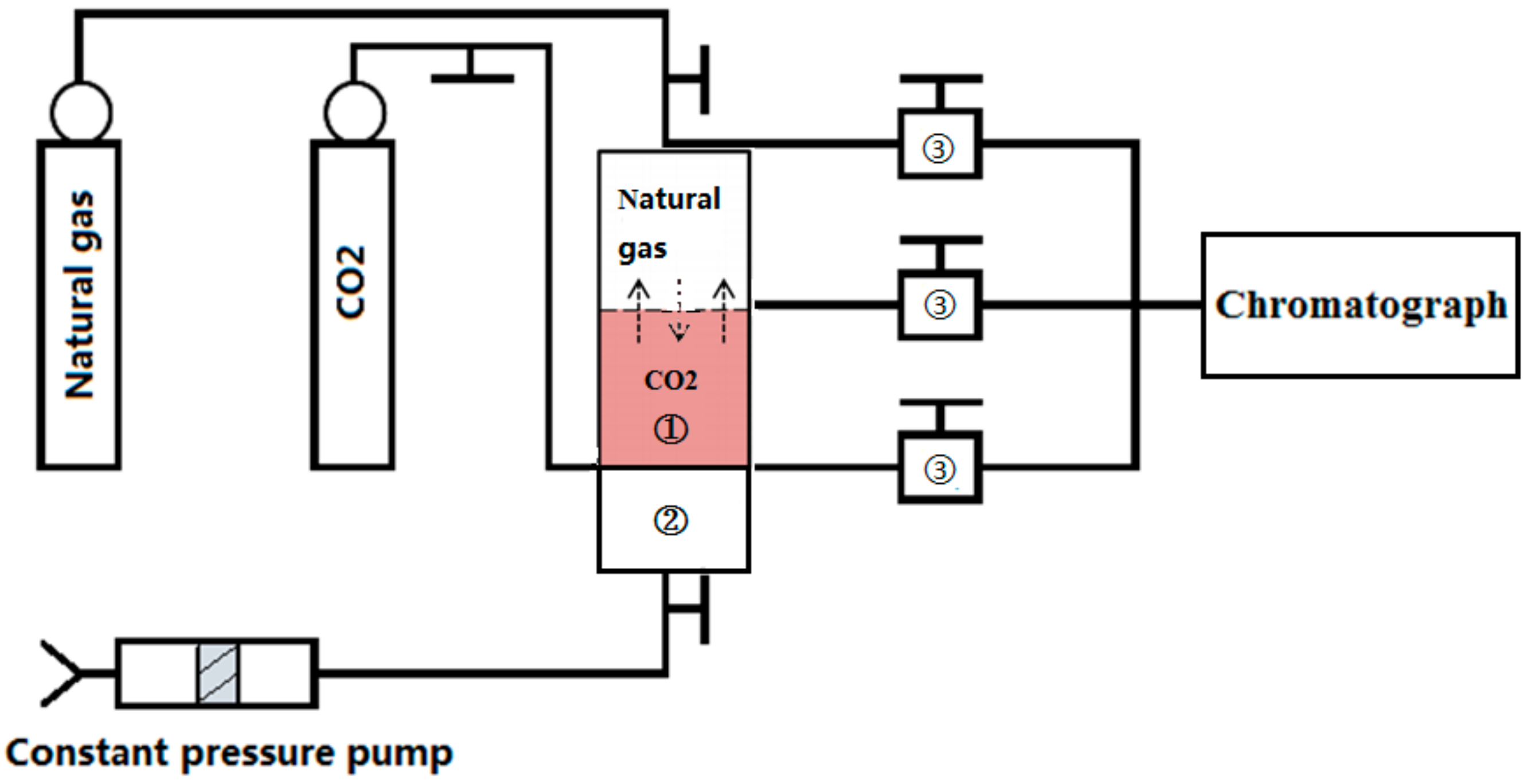
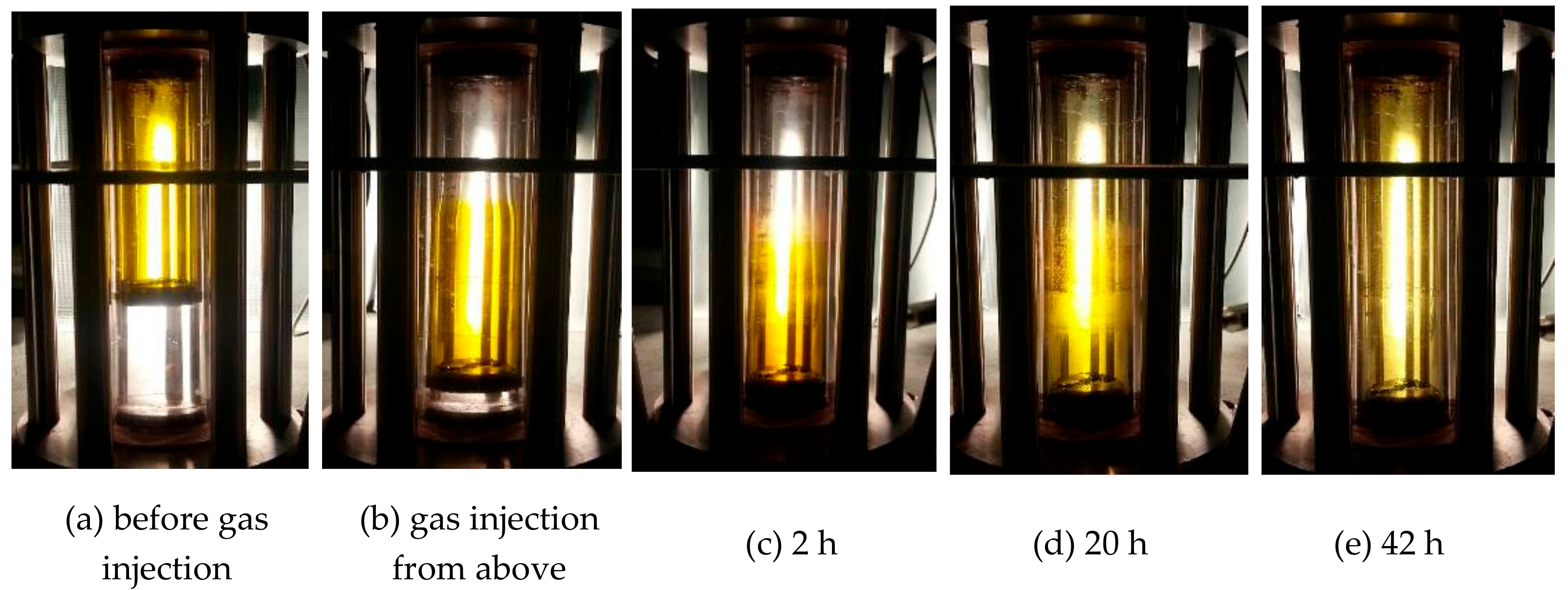
2.1.3. Supercritical CO₂–Natural Gas Diffusion Experiment

The experimental apparatus was designed to measure the diffusion coefficient of CO₂ in natural gas. The experimental apparatus consisted of a high-pressure cell (the upper part) and the pressure control zone (the lower part). An experimental schematic is shown in Figure 5. The high-pressure cell was placed in a constant temperature air bath. The bottom of the high-pressure cell was connected to a high-pressure control zone to maintain pressure throughout the system and was insensitive to overall changes in phase volumes. With the CO₂ contact with natural gas, the high-pressure valve was closed and the contents of the high-pressure cell were allowed to equilibrate over a period of several hours. There were three sampling points placed on the high-pressure cell, which were upper, middle, and lower sampling points. In the experiment, natural gas was injected into the high-pressure cell first with a constant pressure. Then, according to the experimental ratio, CO₂ was injected into the high-pressure cell from the sampling point at the lower part of the device without pressure turbulence to guarantee there was only diffusion in the system. Injecting the higher density and viscosity fluid (CO₂) into the lower density and viscosity natural gas should result in a more stable state. After the start of the diffusion process, samplings were performed simultaneously at the three points while keeping a constant pressure, and then the gas compositions from the three sampling points were measured with chromatographic analysis. The diffusion coefficient was determined using the measured composition data.

2.1.4. Flooding Experiment

The long-core flooding experiments were performed in the HTHP long-core displacement system (Core Laboratories, Tulsa, OK, USA) that allowed core samples to be tested at the reservoir temperature and pressure. Seven pressure measuring points were set from the inlet to the outlet of the sample. The schematic is provided in Figure 6. The gas flow into the core sample was controlled through pumps. The outflow gas was controlled using a backpressure control device with outflow gas, then at atmospheric pressure passing through a flow meter, and then to a gas chromatograph. The experiment was housed in a temperature-controlled cabinet to enable tests to be performed at the reservoir temperature.

The tests were performed on a 25 mm diameter × 1000 mm long sandstone core. First, the core was water-saturated. Gas was used to displace the water and age the core for several hours. After aging, there was no water production with an irreducible water saturation of 37.3%. Then, a depletion test was conducted to simulate the recovery using a multistage pressure drop at an interval of 3 MPa, until 8 MPa was reached. The cumulative recovery was calculated. On this basis, CO₂ was injected at 11 MPa at the inlet and produced at the output at 8 MPa. Throughout the experiment, the gas recovery and gas composition of the outlet were recorded. The CO₂ injection process was performed for more than 1 HCPV (hydrocarbon pore volume) to guarantee that no more natural gas was being produced.

2.2. Numerical Model

2.2.1. Assumptions and Governing Model

The reservoir rock was assumed to be rigid and chemically inert over the timescale of interest (≤20 years), and the reservoir and fluid temperature were assumed to be constant [25]. Advection of gas and liquid phases is governed by a multiphase extension of Darcy’s law. Diffusion of CO₂ in the gas phase is modeled based on diffusion experiment results. The main gas species partition between gas and liquid is modeled based on an adjusted Peng–Robinson equation of state. The three-dimensional, multi-component seepage compositional model is as follows:

$$\begin{gathered} \nabla \left[{\displaystyle \sum _g\frac{k{k}_{rg}}{{\mu }_g}{\rho }_g{y}_{ig}}\nabla {\mathsf{\Phi }}_g^{\ast }\right]+\nabla \left[{\displaystyle \sum _g{\rho }_g{\varphi }_g{S}_g{D}_{ig}\nabla y_{ig}}\right]+{\displaystyle \sum _{k=1}^{n_f}{\displaystyle \sum _g{\rho }_i{q}_{ik}{y}_{ig}}}-\frac{\partial \left[{\displaystyle \sum _g\varphi {\rho }_g{y}_{ig}{S}_g}\right]}{\partial t}=0, \\ i=1,\dots ,n,k=1,\dots ,n \end{gathered}$$

(1)

$$\nabla \left[\frac{k{k}_{rw}}{{\mu }_w}{\rho }_w\nabla p_w\right]+q_w-\frac{\partial \left(\varphi {\rho }_w{S}_w\right)}{\partial t}=0$$

(2)

$$\nabla \left[\frac{K{K}_{\mathrm{rg}}}{{\mu }_{\mathrm{g}}}{\rho }_{\mathrm{g}}\nabla p_{\mathrm{g}}\right]+q_{\mathrm{t}}-\frac{\partial N_{\mathrm{g}}}{\partial t}=0$$

(3)

where, $k$ is the permeability of porous media; $k_r$ is the relative permeability; $\rho$ is the molar density; $y_i$ is the mole fraction of component i in phase; $S$ is the saturation; $D$ is the diffusion factor; $q$ is the flow rate; $i,j$ are the components ($i=1,\dots ,n_c$); $k$ is the phase (o,g,w,s); and Ng is the total number of moles in the gas phase.

Considering the diffusion of CO₂ in gas, the diffusion tensor was used to solve Equation (4):

$$D_{ij}=\left[\begin{array}{ccc}{D}_{ij}^{xx}& D_{ij}^{xy}& D_{ij}^{xz}\\ D_{ij}^{yx}& D_{ij}^{yy}& D_{ij}^{yz}\\ D_{ij}^{zx}& D_{ij}^{zy}& D_{ij}^{zz}\end{array}\right]$$

(4)

where

$$D_{ij}^{xx}=\frac{D_{ij}^{\ast }}{{\tau }_j}+\frac{\left({\alpha }_{j\mathcal{l}}-{\alpha }_{jt}\right)}{\varphi S_j\left|u_j\right|}{u}_{jx}^2+\frac{{\alpha }_{jt}\left|u_j\right|}{\varphi S_j}$$

$$D_{ij}^{yy}=\frac{D_{ij}^{\ast }}{{\tau }_j}+\frac{\left({\alpha }_{j\mathcal{l}}-{\alpha }_{jt}\right)}{\varphi S_j\left|u_j\right|}{u}_{jy}^2+\frac{{\alpha }_{jt}\left|u_j\right|}{\varphi S_j}$$

$$D_{ij}^{zz}=\frac{D_{ij}^{\ast }}{{\tau }_j}+\frac{\left({\alpha }_{j\mathcal{l}}-{\alpha }_{jt}\right)}{\varphi S_j\left|u_j\right|}{u}_{jz}^2+\frac{{\alpha }_{jt}\left|u_j\right|}{\varphi S_j}$$

where, ρ_i is the density of component i, kg/m³; S_j is the saturation of phase j; D_ig is the diffusion coefficient of component i in the gas phase, m²/d; D^*_{i j} is the diffusion coefficient of component i in the gas phase j, m²/d; u_j is the velocity phasor, m²/d; u_jx is the velocity phasor in the x-direction, m²/d; u_jy is the velocity phasor in the y-direction, m²/d; u_jz is the velocity phasor in the z-direction, m²/d; Τ_j is the tortuosity; а_jl is the one-way dispersion coefficient of phase j; and а_jt is the lateral dispersion coefficient of phase j.

CO₂ diffusion coefficients were obtained using theexperimental test results. Reservoirs with different permeabilities were divided into different zones and loaded with different diffusion coefficients

The (2$n_c$ + 2) primary unknowns of the above models are $p;N_1,N_2,\dots ,N_{n_{\mathrm{c}}};N_{\mathrm{w}};N_{1\mathrm{g}},N_{2\mathrm{g}},\dots ,N_{n_{\mathrm{c}}\mathrm{g}}$. To calculate these unknowns, the above ($n_c$ + 2) equations are not adequate. Thus, an equilibrium equation, supplement equation, and definite condition were added, which are given as follows.

2.2.2. Equilibrium Equation

The equilibrium equation of each component:

$$\ln f_{ig}=\ln f_{io}, i=1,\dots ,n_c$$

(5)

where $f$ is the fugacity.

$K_{ig}$ ($i=1,\dots ,n_c$) and $f_g$ can be calculated using an adjusted multiphase equilibrium model during supercritical CO₂ injection, which is proposed as follows:

$$V_1+V_2+L=1$$

(6)

$$V_1{x}_{iv1}^{}+V_2{x}_{iv2}^{}+L{x}_{il}^{}=z_i$$

(7)

$${\displaystyle \sum _{i=1}^n{x}_{iv1}^{}={\displaystyle \sum _{i=1}^n{x}_{iv2}^{}=}{\displaystyle \sum _{i=1}^n{x}_{il}^{}=}}{\displaystyle \sum _{i=1}^n{z}_i^{}=1}$$

(8)

where $f$ is the fugacity, $V_1$ is the mole fraction of gas phase with rich CO₂, $V_2$ is the mole fraction of natural gas phase, $L$ is the mole fraction of liquid phase, $x_i$ is the molar concentration of in different phases, $z_i$ is the molar concentration of in the whole system, $v1$ denotes the gas phase with rich CO₂, $v2$ denotes the gas phase, and $l$ denotes the liquid phase.

Characterization of the supercritical CO₂-vapor components:

$$f_{iv1}=x_{iv1}{\phi }_{iv1}p$$

(9)

$$f_{iv2}=x_{iv2}{\phi }_{iv2}p$$

(10)

where $\phi$ is the fugacity coefficient.

In this work, the adjusted Peng–Robinson equation of state was used.

Adjusted Peng–Robinson Equation of State

The Peng–Robinson equation of state was adjusted because the experimental thermodynamic parameter could not be fitted well with EOS especially near the critical temperature and critical pressure. There were two terms that neededadjusting. One is volume correction term of critical point, and the other is the volume correction term considering the temperature influence:

$$c\left(T\right)=c_{c}f\left(T_r\right)$$

(11)

where $c\left(T\right)$ is the critical volume adjusted term, $c_c$ is the volume correction term of critical point, and $f\left(T_r\right)$ is the volume correction term considering temperature influence.

The volume correction term of the critical point was adjusted with experiment data as follows:

$$c_c=v_{EOS}-v_{E\mathrm{xp}}=\left(0.3074-Z_c\right)\frac{R{T}_c}{P_c}$$

(12)

where $Z_c$ is the critical compression factor, $\mathrm{R}$ is the universal gas constant, $T_c$ is the critical temperature, $p_c$ is the critical pressure, $v_{EOS}$ is the molar volume calculated by EOS, and $v_{E\mathrm{xp}}$ is the molar volume calculated via experiment.

In addition, especially near the critical temperature, the thermodynamic parameter could not be fitted well. Thus, atemperature-adjusted term was added through the relationship between $Z_c$ and temperature. The referenced experiment test result is shown as Figure 7. The formula can be presented as follows:

$$f\left(T_r\right)=\beta +\left(1-\mathsf{\beta }\right)\exp \left(0.5\beta +8.3\right)$$

(13)

$$\beta =-2.8431\exp \left(\left[-64.2184\left(0.3074-{\mathrm{Z}}_c\right)\right]+0.1735\right)$$

(14)

$$\beta =T-T_r$$

(15)

where $T$ is the temperature, $T_r$ is the $T/T_c$ relative temperature, and $\beta$ is the temperature correction term.

3. Results and Analysis

3.1. Experiment Results and Analysis

3.1.1. Non-Equilibrium Experiment

The non-equilibrium experiment was carried out in a high-pressure visualization device. The experimental temperature was 35 °C. During the experiment, CO₂ with a dyeing agent was injected into the device, and then the natural gas was injected from the upper part under constant pressure with 9 MPa. The non-equilibrium phase behavior after CO₂ contact with natural gas is shown in Figure 8.

The non-equilibrium experiment of CO₂ and natural gas snapshots revealed the obvious phase behavior change between CO₂ and natural gas around the critical point (Figure 8). First, the pure CO₂ was pumped into the device, which is displayed in yellow in the upper part of the piston after dyeing (Figure 8a). The lower part of the device was the pressurized medium (water). Then, gas was pumped into the device at the upper part, which was shown in Figure 8b. It could be clearly seen that natural gas was colorless and transparent, which was totally different from the CO₂ with a yellow color, and a clear interface was exhibited between two fluids. After mixing, the experiment was stood still for 2 h and the interface between the two gases gradually blurred. After the mix experiment was stood still for 20 h, the upper part was pale yellow and the lower part was dark yellow, indicating CO₂ had moved upward, but the two gases were still not uniformly mixed. When the diffusion time had reached 42 h, the color of the system was light yellow and uniform, indicating that the two gases were completely mixed.

Overall, the non-equilibrium experiment proved that there was weak diffusion between supercritical CO₂ and natural. The supercritical CO₂ in the gas reservoir did not rapidly mix with natural gas to form a phase, which is beneficial to enhance gas recovery via CO₂ flooding.

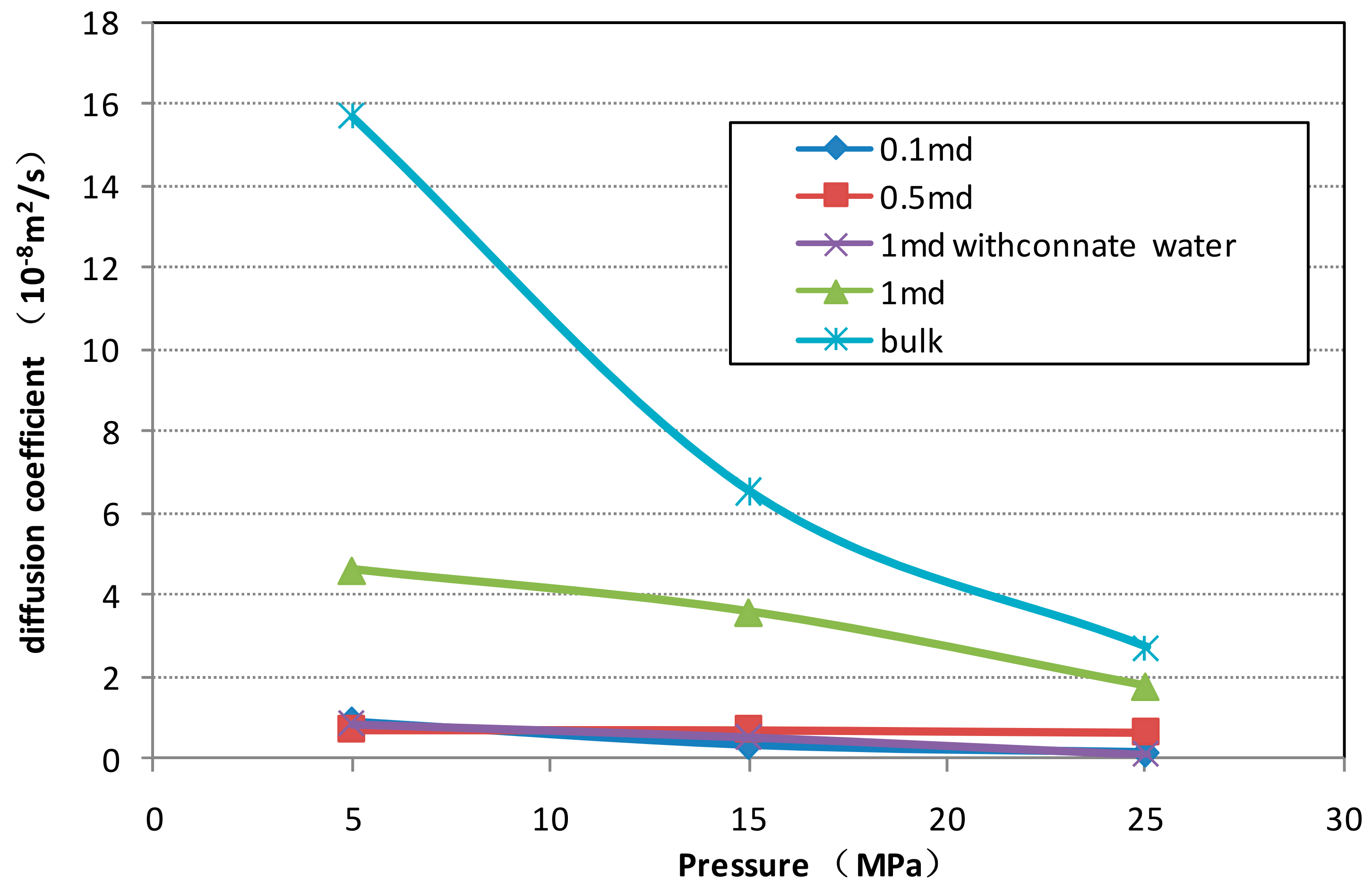
3.1.2. Diffusion Experiment

Series experiments were conducted for calculating the diffusion coefficient of the CO₂ and natural gas mixing process under different pressure conditions with bulk and porous media. The test results are given in Figure 9, which show that as the pressure increased, the diffusion coefficient gradually decreased. As the core permeability increased, the diffusion coefficient increased gradually. When there was connate water in porous media, the diffusion coefficient of CO₂ in natural gas decreased. Diffusion experiments show that the mix degree between CO₂ and natural gas was not severe, which could form a narrow miscible zone to achieve effective CO₂ displacement.

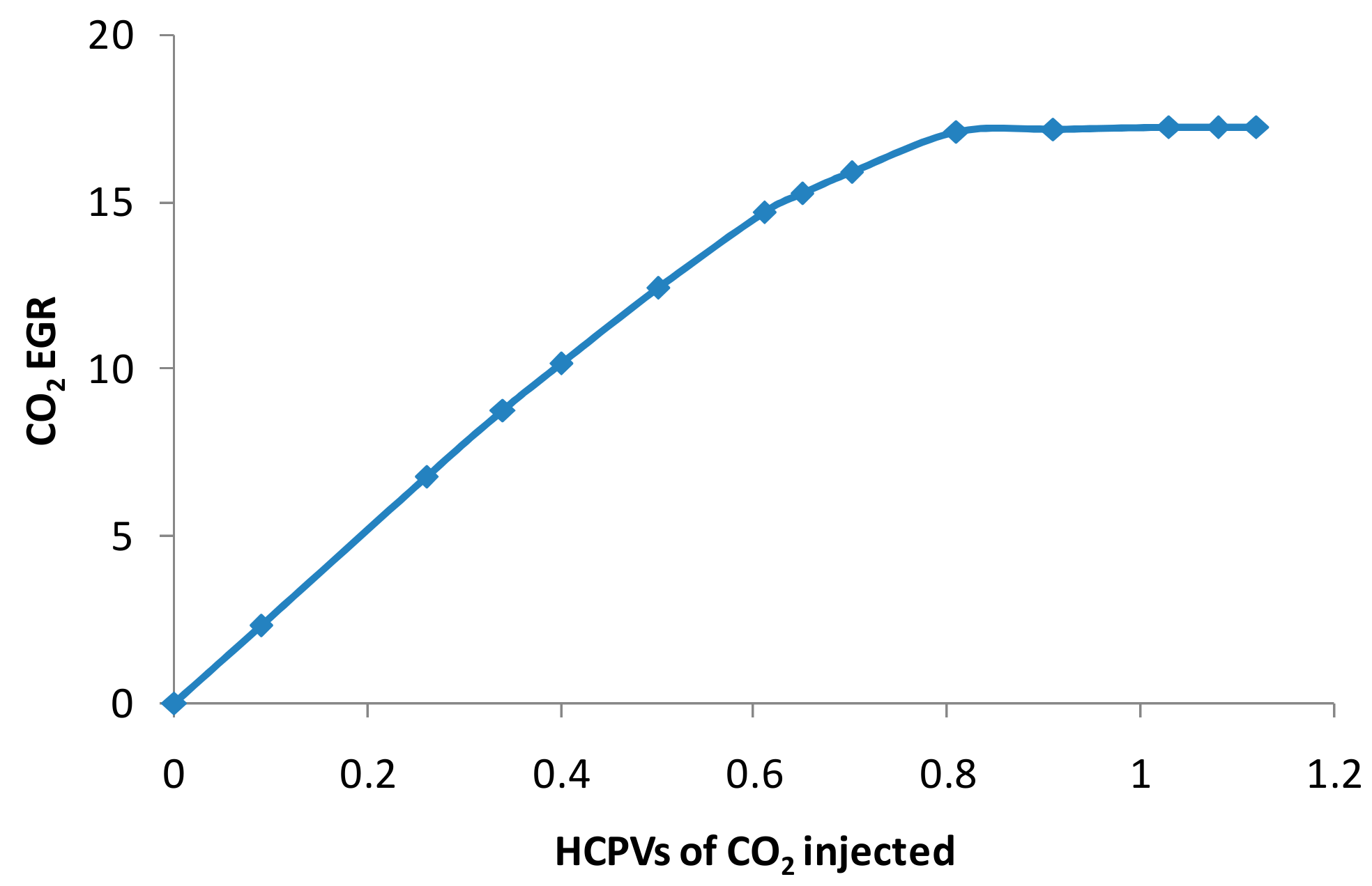
3.1.3. Long Core Model

In the long core experiment, the cumulative recovery was 47.6% in the natural gas depletion development process. The observed CO₂ mole percentage at the outlet and enhanced gas recovery from the long core experiment are presented in Figure 10 and Figure 11. When the volume of the injected CO₂ was 0.5 HCPV, the CO₂ mol% in the gas at the outlet was 10%, which is the point that can be deemed as the break through point. As more HCPVs of supercritical CO₂ were injected, the initial recovery increased linearly. When 0.6 HCPV was injected, the increasing rate of the recovery decreased. When more than 0.8 HCPV was injected, the recovery remained almost unchanged.The total amount of gas recovery increased by 17.3% after the depletion recovery. When the CO₂ content at the outlet was 10% (at low cost of corrosion), the CO₂ EGR was 12%. This result shows that supercritical CO₂ can effectively displace natural gas and it is a technically feasible method.

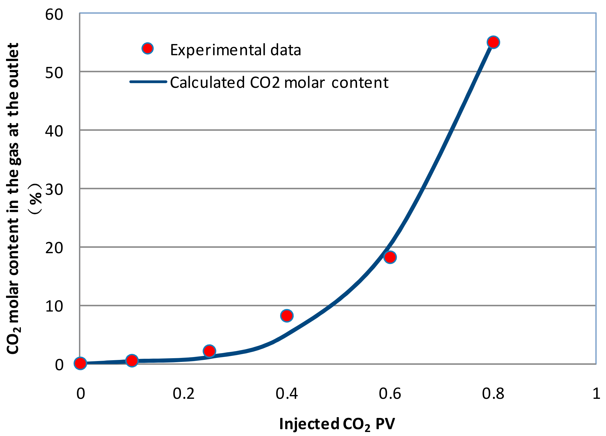
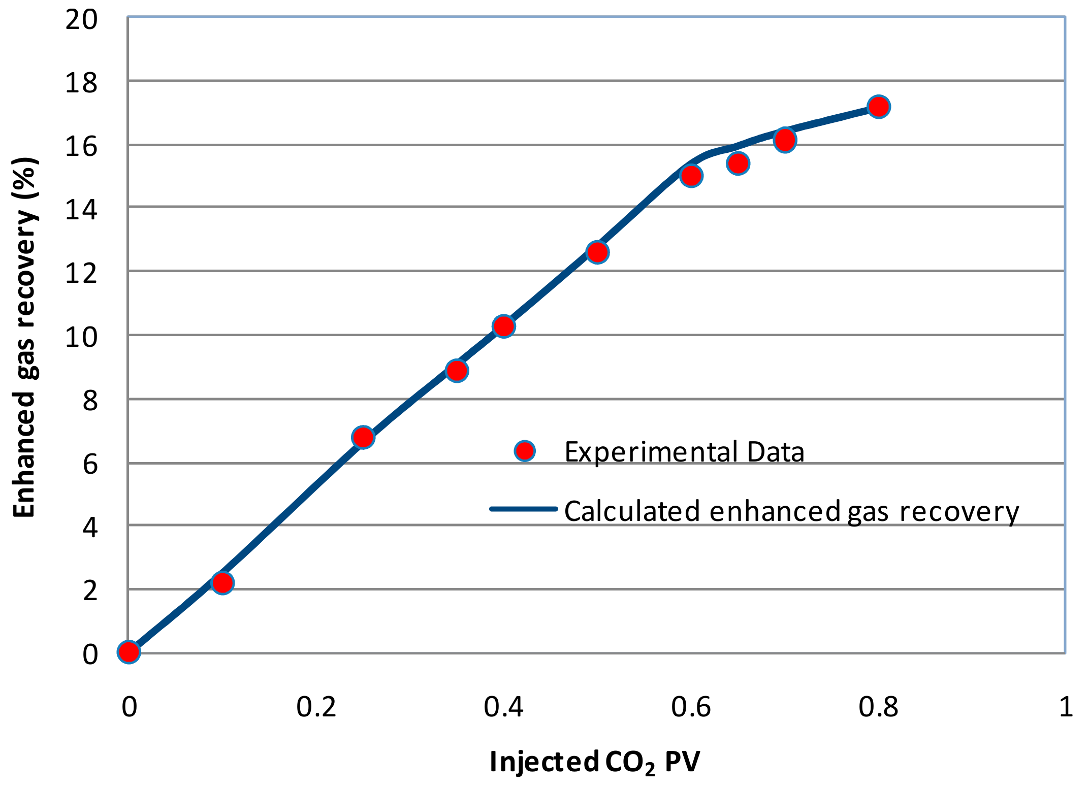
3.2. Numerical Model Verification

Using the above equations, the numerical model was established and then experimental data were calculated. The fitting error with the experimental value was less than 5% (see Figure 12 and Figure 13).

3.3. CO₂ EGR Mechanism

Based on the experiment, the numerical simulation method was used to investigate the natural gas displacement mechanism via CO₂ flooding.

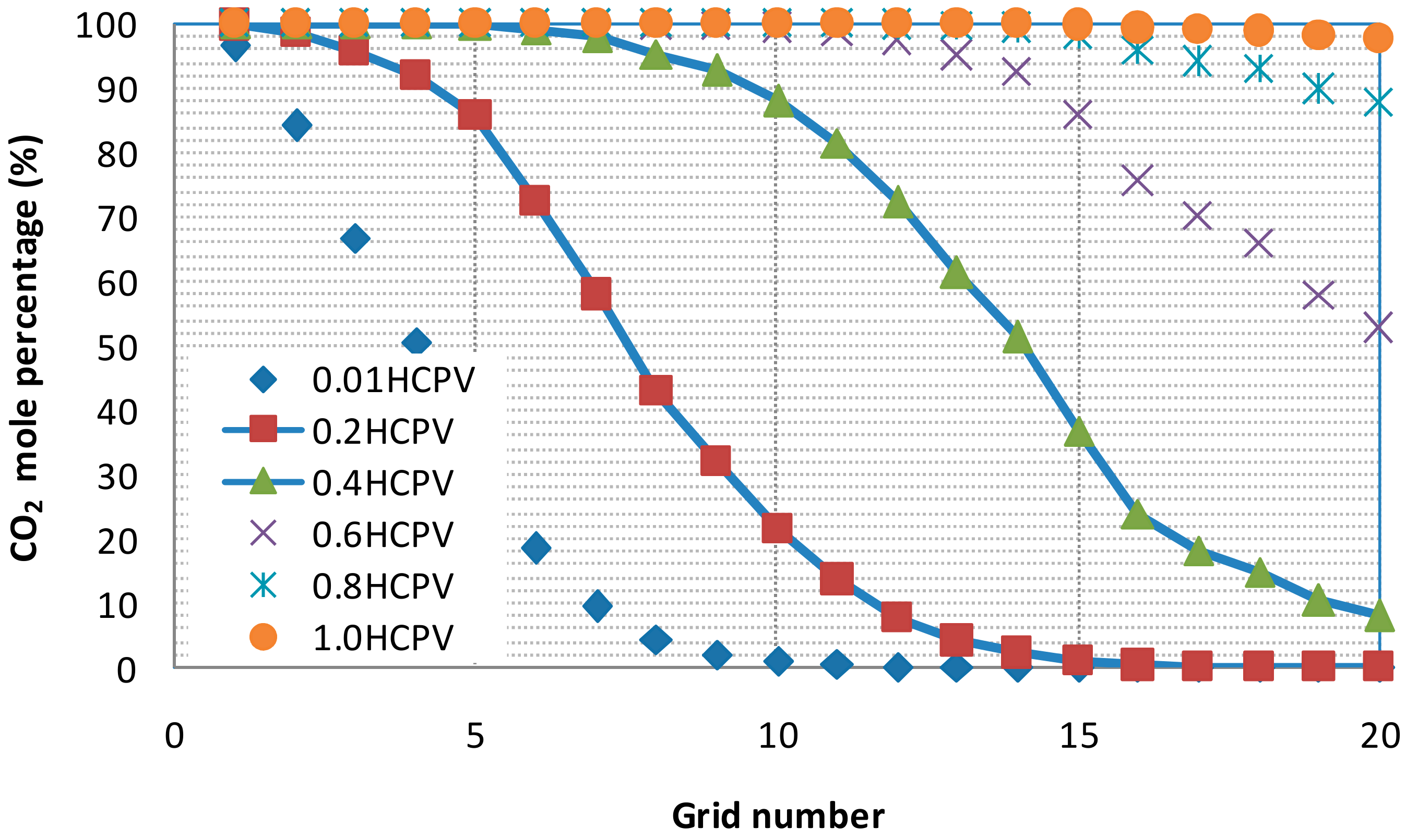
3.3.1. Partial Miscibility

Non-equilibrium and diffusion experiments proved that there was a weak diffusion between supercritical CO₂ and natural gas. The supercritical CO₂ in the gas reservoir did not rapidly mix with natural gas to form one phase.

(1) Long Core Model

Simulations of the long core model and dip model were established to certify that the partially miscible feature existed between CO₂ and natural gas. The long core model had 20 grids in the horizontal direction and one layer in the vertical direction (Figure 14). The layer in the vertical direction had a thickness of 5 cm. In the horizontal direction, CO₂ was injected at the first grid, and gas was produced at the 20th grid. The average permeability was 0.652 mD, the porosity was 9.9%, and the residual water saturation was 37.3%. The initial pressure and temperature used in the model was based on the DND gas field (p_i = 25 MPa, T = 85 °C)

Shown in Figure 15 are profiles of the CO₂ mole fraction in the gas in each grid at six different CO₂ HCPV injections during the CO₂ flooding. Figure 16 shows the corresponding CO₂ density for the same simulation. The gas density varied from just below 200 kg/m³ to just around 600 kg/m³, where CO₂ was in a supercritical state. At the initial stage of injection (0.01 HCPV), the CO₂ at the injection end (first grid) was not miscible with natural gas, which exhibited supercritical characteristics; the 10th grid was the displacement front; and between the second and tenth grid, the CO₂ concentration decreased, showing a partially miscible mixed feature. After the constant CO₂ injection, the frontier of CO₂ flooding advances continuously. With the continuous mixing of natural gas, the density of the mixed belt was gradually reduced and the density of the displacement front was close to that of the gas. This further confirmed that there was no mixture between CO₂ and natural gas on a large scale.

(2) Dip Model

In order to further study the mixing process of CO₂ and natural gas in the CO₂ flooding process, a single-injection production model was established. The model had 80 grids in the horizontal direction and 10 layers in the vertical direction. The number of grids was 80 × 10 = 800. The thickness of each layer in the horizontal direction was 1 m. In the horizontal direction, one injection well was set in the first grid, and one production well was located in the 80th grid. The distance between production well and the injection well was 800 m. The longitudinal permeability was set to 0.1 mD, the porosity was set to 8%, and the irreducible water saturation was 35%. CO₂ was injected into the lower region of the reservoir while natural gas was produced from the upper region.

We present in Figure 17 and Figure 18 the simulation results for CO₂ density and viscosity after around 1month of injection and production. From the simulation results, after injecting the CO₂, it had the highest concentration near the gas injection well, and its concentration decrease dduring contact with the natural gas. The density maps and viscosity maps (Figure 11 and Figure 12) in the horizontal direction (represented by k = 1–10, 1 represents first upper layer, 10 represents the tenth layer) indicate that near the injection end, the fluid properties of the mixture at the injection end displayed supercritical CO₂ characteristics, while at the displacement front, the mixture exhibited gaseous features.

In summary, the density variation and the viscosity change of each grid in the dip model indicated that there were three zones during CO₂ flooding: the CO₂ flooding frontier, the partial mixture zone between CO₂ and natural gas, and the supercritical CO₂ zone.

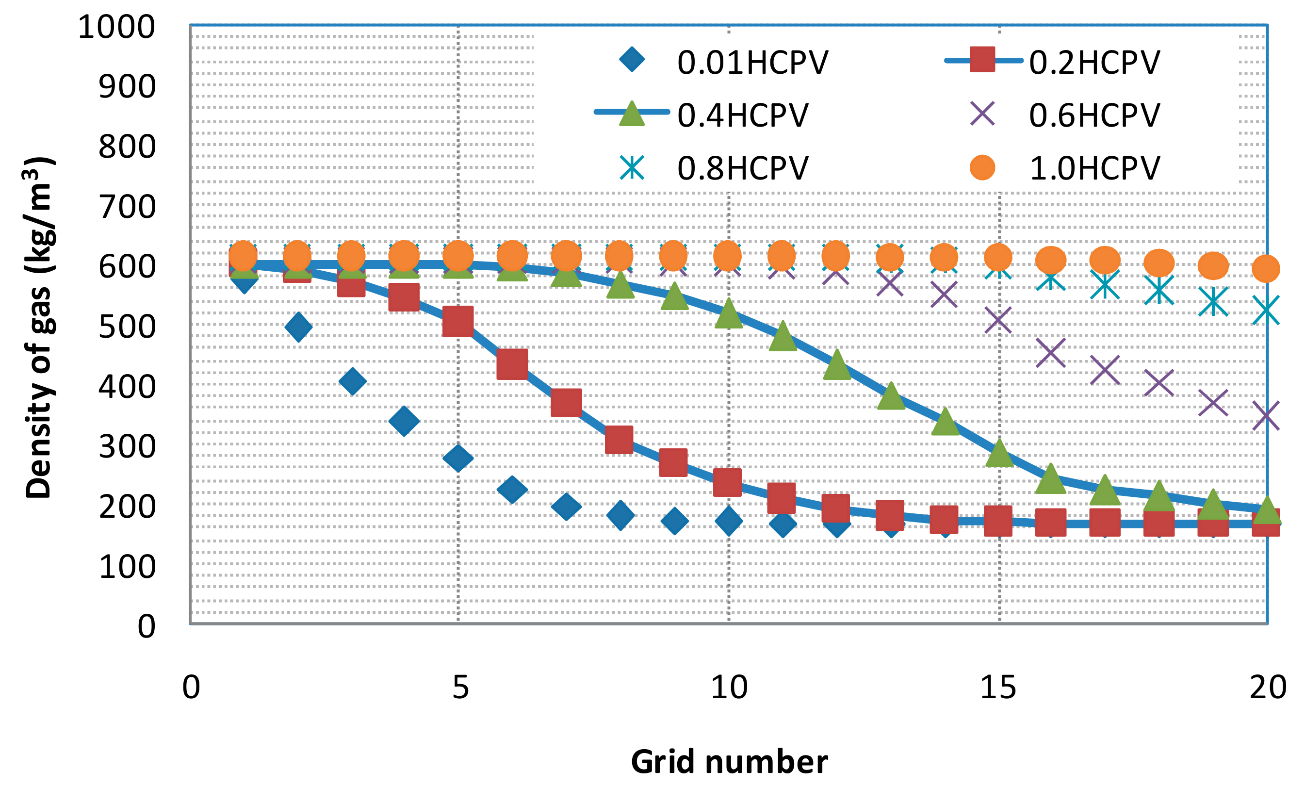
3.3.2. Pressure Maintenance

Simulations of an idealized two-dimensional gas reservoir with CO₂ flooding have been carried out with the anticline model. The idea here is that after natural depletion, the reservoir could be used for CO₂ flooding with pressure maintenance to enhance gas recovery (see Figure 19). CO₂ was injected in the lower left-hand and right-hand corner of the model domain, while natural gas was produced in the upper side in the middle of the model domain. The model had 53 grids in the horizontal direction and 50 layers in the vertical direction. The thickness of each layer in the vertical direction was 20 cm. The distance between the production well and the injection well was 800 m. The permeability was set to 0.1 mD, the porosity was set to 8%, and the irreducible water saturation was 35%. After natural depletion, the pressure of the reservoir dropped to 100 bar and CO₂ was used for injection. Figure 19 shows the reservoir pressure increase after CO₂ flooding. The simulation results indicate that mixing with CO₂ promoted the migration of natural gas to the high part from the bottom of the reservoir, where the pressure of the entire gas reservoir rose.

3.3.3. Cushion Gas Mechanism

Critical to the use of CO₂ EGR is the idea of a cushion gas, i.e., CO₂ whose compression allows for additional storage of natural gas, and whose expansion helps drive production of natural gas. A schematic showing CO₂ cushion gas is shown in Figure 20. The cushion gas was CO₂. CO₂ that was compressed through its critical pressure near the critical temperature was a very effective cushion gas because of its large compressibility. There was a smaller value of Z for CO₂ than that of natural gas. Thus, the CO₂ cushion gas allowed more gas to be stored. The simulation results show that due to the effect of gravity differentiation, CO₂ will accumulate in the lower part of the gas reservoir. Because the reservoir was under a supercritical condition, CO₂ had supercritical characteristics, where CO₂ had a much denser and was more viscous than pure CH₄ in the gas reservoirs. The difference in physical properties between CO₂ and CH₄ strongly favored supercritical CO₂ under riding natural gas to achieve natural gas displacement and CO₂ sequestration (Figure 20).

4. Conclusions

A novel phase behavior experimental device with a screened supercritical CO₂ dyeing agent were first presented to understand the effect of supercritical CO₂ on the phase behavior properties of natural gas. The mass transfer between two vapor phases was also measured. Based on experimental results, the compositional model considering the influence of CO₂ diffusion on the gas recovery and critical property adjustment of supercritical CO₂ was established. Through the establishment of fluid phase experiments with CO₂ flooding gas and numerical evaluation method, three CO₂ mechanisms were recognized:

(1) Partial Mixture

Non-equilibrium and diffusion experiments proved that there was a weak diffusion between supercritical CO₂ and natural gas. Meanwhile, the dip model also indicated that there were three zones during CO₂ flooding: CO₂ flooding frontier, the partial mixture zone between CO₂ and natural gas, and the supercritical CO₂ zone. The supercritical CO₂ in the gas reservoir didnot rapidly mix with natural gas to form onephase.

(2) Pressure Maintenance

Injected CO₂ raised the pressure of the entire gas reservoir.

(3) Cushion Driving

The difference in physical properties between CO₂ and CH₄ strongly favor supercritical CO₂ under riding natural gas to achieve natural gas displacement and CO₂ sequestration, which is similar to the proven cushion gas used in the gas storage industry wherein the expansion of cushion gases upon natural gas withdrawal aids in production from the storage reservoir.

Experiment and reservoir simulation studies show favorable results for CO₂ EGR, which is seen as a promising way of prolonging the productive life and enhancing recovery of tight gas reservoirs.

References

1. Sheng, P.P.; Liao, X.W. The Technology of Carbon Dioxide Stored in Geological Media and Enhanced Oil Recovery, 1st ed.; Petroleum Industry Press: Beijing, China, 2009; pp. 1–4. [Google Scholar]
2. IEA. Carbon Dioxide Utilization; Table 6; IEA Greenhouse Gas R&D Programme: Paris, France, 1997. [Google Scholar]
3. Wang, H.; Ma, F.; Tong, X.; Liu, Z.; Zhang, X.; Wu, Z.; Li, D.; Wang, B.; Xie, Y.; Yang, L. Assessment of global unconventional oil and gas resources. Pet. Explor. Dev. 2016, 43, 850–862. [Google Scholar] [CrossRef]
4. Jia, A.L. Progress and prospects of natural gas development technologies in China. Nat. Gas Ind. 2018, 38, 77–86. [Google Scholar] [CrossRef]
5. Ma, X.H.; Jia, A.L.; Tan, J. Tight sand gas development technologies and practices in China. Pet. Explor. Dev. 2012, 39, 572–579. [Google Scholar] [CrossRef]
6. Zou, C.N.; Yang, Z.; He, D.B. Theory, technology and prospects of conventional and unconventional natural gas. Pet. Explor. Dev. 2018, 45, 575–587. [Google Scholar] [CrossRef]
7. Yuan, S.Y.; Wang, Q. New progress and prospect of oilfields development technologies in China. Pet. Explor. Dev. 2018, 45, 657–668. [Google Scholar] [CrossRef]
8. Yuan, S.Y. Symposium of Gas Drive to Improve Oil Recovery, 1st ed.; Petroleum Industry Press: Beijing, China, 2016; pp. 1–15. [Google Scholar]
9. Oldenberg, C.; Pruess, K.; Benson, S. Process modeling of CO2 injection into natural gas reservoirs for carbon sequestration and enhanced gas recovery. Energy Fuels 2001, 15, 293–298. [Google Scholar] [CrossRef]
10. Oldenberg, C.; Benson, S. CO2 injection for Enhanced Gas Production and Carbon Sequestration. In Proceedings of the SPE International Petroleum Conference an Exhibition, Villahemosa, Mexico, 10–12 February 2002. SPE 74367. [Google Scholar]
11. Sun, Y. Mechanism of Superciritical-CO2 Storage with Enhanced Gas Recovery in the Natural Gas Reservoirs. Ph.D. Thesis, Southwest Petroleum University, Chengdu, China, 2012. [Google Scholar]
12. Dali, H.; Lihui, G.; Haocheng, L.; Meizhu, Z.; Feifei, C. Dynamic phase behavior of near-critical condensate gas reservoir fluids. Nat. Gas Ind. 2013, 33, 68–73. [Google Scholar]
13. Mamora, D.D.; Seo, J.G. Enhanced gas recovery by carbon dioxide sequestration in depleted gas reservoir. In Proceedings of the SPE Annual International Petroleum Conference, San Antonio, TX, USA, 29 September–2 October 2002. [Google Scholar]
14. Tang, Y.; Zhang, C.; Du, Z.M.; Cui, S.H.; Ma, Y.X.; Mi, H.G. Experiments on enhancing gas recovery and sequestration by CO2 displacement. Reserv. Eval. Dev. 2015, 5, 34–49. [Google Scholar]
15. Nogueira, M.C.; Mamora, D.D. Effect of Flue Gas Impurities on the Process of Injection and Storage of CO2 in Depleted Gas Reservoirs. In Proceedings of the 2005 SPEBPA/DOE Exploration and Production Environmental Conference, Galveston, TX, USA, 7–9 March 2005. [Google Scholar]
16. ATTurta, S.S.K.; Sim, A.K.; Singhal, B.F.; Hawkins, A. Basic investigation on enhanced gas recovery by gas-gas displacement. In Proceedings of the Petroleum Society’s 8th Canadian International Petroleum Conference, Calgary, AB, Canada, 12–14 June 2007. [Google Scholar]
17. Shi, Y.; Jia, Y.; Pan, W.; Huang, L.; Yan, J.; Zheng, R. Potential Evaluation on CO2-EGR in tight and low permeability reservoirs. Nat. Gas Ind. 2017, 37, 62–69. [Google Scholar]
18. Clemens, T.; Secklehner, S.; Mantatzis, K.; Jacobs, B. Enhanced Gas Recovery, Challenges shown at the Example of three Gas Fields. In Proceedings of the SPE EUROPEC/EAGE Annual Conference and Exhibition, Barcelona, Spain, 14–17 June 2010. [Google Scholar]
19. Al-Hasami, A.; Ren, S.; Tohidi, B. CO2 Injection for enhanced gas recover and geo-storage: Reservoir simulation and economics. In Proceedings of the SPE EUROPEC/EAGE Annual Conference, Madrid, Spain, 13–16 June 2005. [Google Scholar]
20. Rafiee, M.M.; Ramazanian, M. Simulation Study of Enhanced Gas Recovery Process Using a Compositional and a Black Oil Simulator. In Proceedings of the SPE Enhanced Oil Recovery Conference, Kuala Lumpur, Malaysia, 19–21 July 2011. [Google Scholar]
21. Van der Meer, L.G.; Kreft, E.; Geel, C.R.; D’Hoore, D.; Hartman, J. CO2 storage and testing enhanced gas recovery in the K12-B reservoir. In Proceedings of the 23rd World Gas Conference, Amsterdam, The Netherlands, 5–9 June 2006. [Google Scholar]
22. Kubus, P. CCS and CO2-Storage Possibilities in Hungary. In Proceedings of the SPE International Conference on CO2 Capture, Storage, and Utilization, New Orleans, LA, USA, 10–12 November 2010. [Google Scholar]
23. Mathieson, A.; Midgley, J.; Dodds, K.; Wright, I.; Ringrose, P.; Saoul, N. CO2 Sequestration Monitoring and Verification Technologies Applied at Krechba, Algeria. Leading Edge 2010, 29, 216–222. [Google Scholar] [CrossRef]
24. Mathieson, A.; Midgely, J.; Wright, I.; Saoula, N.; Ringrose, P. In Salah CO2 Storage JIP: CO2 sequestration monitoring and verification technologies applied at Krechba, Algeria. Energy Procedia 2010, 1063, 1–8. [Google Scholar] [CrossRef]
25. Turgay, E.; Jamal, H.A.; Gregory, R.K. Basic Applied Reservoir Simulation—SPE Text Book Series Vol. 7, 1st ed.; Society of Petroleum Engineers Inc.: Houston, TX, USA, 2001; pp. 387–395. [Google Scholar]
Figure 1. The distribution of conventional-unconventional gas reservoirs in China [6].
Energies 12 02225 g001
Figure 2. High pressure visualization device for qualitative observation of non-equilibrium phase experiment.
Energies 12 02225 g002
Figure 3. Supercritical CO2 Dyeing agent.
Energies 12 02225 g003
Figure 4. CO2 dyeing effect under different pressures at 35 °C (from left to right the pressure increased from 5 MPa to 14 MPa).
Energies 12 02225 g004
Figure 5. The schematic of CO2-gas diffusion experiment including: ① high-pressure cell, ② pressure control zone, and ③ sampling points (in this experiment, the distance between the upper-middle sampling point and the lower-middle sampling point was half of the height of the high-pressure cell, namely 27.5 cm).
Energies 12 02225 g005
Figure 6. Experimental set-up of HPHT long-core displacement system for CO2 flooding experiment.
Energies 12 02225 g006
Figure 7. The relationship between Z c and β . Dots represent the experiment data of β with different Z c . The solid line is the experimental data fitting line.
Energies 12 02225 g007
Figure 8. Visualization results of non-equilibrium phase behavior of CO2 and natural gas at 9 MPa.
Energies 12 02225 g008
Figure 9. Relationship between the diffusion coefficient of CO2 in natural gas and pressure with different permeabilities (blueline with diamonds represents the diffusion coefficient of CO2 in 0.1 md porous media, redline with squares represents the diffusion coefficient of CO2 in 0.5 md porous media, purple line with crosses represents the diffusion coefficient of CO2 in 1 md porous media, green line with triangles represents the diffusion coefficient of CO2 in 1 md porous media with connate water, and blueline with stars represents the diffusion coefficient of CO2 in bulk media).
Energies 12 02225 g009
Figure 10. Variation in CO2 mol% at the outlet during CO2 injection in the long core experiment.
Energies 12 02225 g010
Figure 11. Profile of enhanced gas recovery versus the amount of HCPVs of CO2 injected obtained in the long core experiment.
Energies 12 02225 g011
Figure 12. Relationship between injected CO2 pore volume (injected CO2 PV) and CO2 molar content at the outlet end. A line has been fitted with the numerical model established in the article.
Energies 12 02225 g012
Figure 13. Relationship between the injected CO2 pore volume (injected CO2 PV) and enhanced gas recovery. A line has been fitted with the numerical model established in the article.
Energies 12 02225 g013
Figure 14. The simulation model of the CO2 long core experiment.
Energies 12 02225 g014
Figure 15. Variation of the mole fraction of CO2 in each grid at different CO2 HCPV injections (blue diamonds represent the mole fraction of CO2 in each grid when 0.01 HCPV CO2 was injected, blueline with red squares represents the mole fraction of CO2 in each grid when 0.2 HCPV CO2 was injected, blueline with green triangles represents the mole fraction of CO2 in each grid when 0.4 HCPV CO2 was injected, purple crosses represent the mole fraction of CO2 in each grid when 0.6 HCPV CO2 was injected, blue stars present the mole fraction of CO2 in each grid when 0.8 HCPV CO2 was injected, and orange circles represent the mole fraction of CO2 in each grid when 1.0 HCPV CO2 was injected).
Energies 12 02225 g015
Figure 16. Variation of gas density in each grid at different CO2 HCPV injections(blue diamonds represent the gas density in each grid when 0.01 HCPV CO2 was injected, blueline with red squares represents the gas density in each grid when 0.2 HCPV CO2 was injected, blueline with green triangles represents the gas density in each grid when 0.4 HCPV CO2 was injected, purple crosses represent the gas density in each grid when 0.6 HCPV CO2 was injected, blue stars represent the gas density in each grid when 0.8 HCPV CO2 was injected, and orange circles present the gas density in each grid when 1.0 HCPV CO2 was injected).
Energies 12 02225 g016
Figure 17. Variation of CO2 density in each grid after around 1month of CO2 injection (k represents the vertical layers, 1 represents thefirst upper layer, 10 represents the tenth layer).
Energies 12 02225 g017
Figure 18. Variation of viscosity in each grid around 1month of CO2 injection (k represents vertical layers, 1 means first upper layer, 10 means the tenth layer).
Energies 12 02225 g018
Figure 19. Pressure flow line distribution diagram in the anticline model.
Energies 12 02225 g019
Figure 20. Schematic of the CO2 “gas cushioning” mechanism diagram.
Energies 12 02225 g020