Research on Evaluation of Power Supply Capability of Active Distribution Network with Distributed Power Supply with High Permeability

Abstract

With the large number of distributed generation (DG) access to the distribution network, the traditional distribution network with a single-supply radial structure has been transformed into an active distribution system (ADS) with source and bidirectional currents. This transformation makes the calculation of the power supply capacity (PSC) of the ADS face new challenges, and the uncertainty of the DG output increases the difficulty in calculating the PSC. At the same time, the power market transaction check needs to meet the safety constraints of the distribution network operation, and is required to know the PSC information of the ADS more quickly and accurately. Therefore, in order to quickly evaluate the PSC of the ADS, this paper proposes a fast evaluation method of the PSC based on the DG output rolling prediction and the information gap decision theory (IGDT). The method first establishes a rolling prediction model of the DG output, and calculates the PSC of the ADS at the corresponding time. Next, it establishes a risk avoidance model (RAM) and a risk speculation model (RSM) for the PSC of the ADS based on the IGDT. These models further calculate the probability of the range of the PSC at the corresponding time, so as to better evaluate the PSC of the ADS. Finally, the improved IEEE-14 node is used to verify that the model can consider the influence of the DG output uncertainty and quickly calculate the information of PSC.

1. Introduction

In recent years, the distributed generation (DG) industry has experienced rapid growth due to its broad prospects in addressing energy demand and environmental issues. After the explosive growth of China’s photovoltaic industry in 2017, by the end of June 2018, the installed capacity of photovoltaic power generation in the country reached 154.51 million kilowatts, of which distributed photovoltaics were 41.9 million kilowatts, and the cumulative grid-connected capacity reached 171.6 million kilowatts [1]. In the “Clean Energy Absorption Action Plan” document issued by China, the decentralized and distributed renewable energy development is clearly prioritized, hence, the penetration rate of the DG on the distribution network side will continue to increase.

The uncertainty and volatility of the DG output lead to frequent changes in the operating state of the active distribution system (ADS). With the increase of the proportion of DG access, the safe and stable operation of the ADS faces greater challenges. At present, there is much research on the ultimate transmission power of transmission lines in the transmission network, and they are relatively mature. However, there are few studies on the power supply capacity (PSC) of distribution networks. The only research is to calculate the substation capacity ratio and the average line load rate. The technical indicators provide a general qualitative assessment of the PSC of the ADS [2,3,4,5], which can provide some guidance for the planning or upgrading of the distribution network, but there is insufficient support for real-time operation control decision-making of the distribution network. There are relatively few studies considering the influence of the DG on the PSC of the ADS. Reference [6] proposes a two-layer optimization model for the maximum PSC of the ADS based on chance constrained programming. Using the opportunity constrained programming, the output of the DG with uncertainty is treated as a random variable. However, the DG output is not completely uncertain. The short-term prediction method can be used to roughly determine the DG output range. Reference [7] proposes an evaluation method for the PSC of the ADS considering reliability flexible demand and post-fault load response. By establishing a photovoltaic annual output forecasting model for the whole year, the sampling error of the predicted values is superimposed to obtain the full-year Photovoltaic (PV) output. This method fails to analyze the influence of the DG output fluctuation on the PSC. Therefore, this paper hopes to further analyze the uncertainty of the DG output and the impact on the PSC by combining the rolling prediction algorithm and information gap decision theory (IGDT) theory.

With the acceleration of the construction of China’s electricity market, the reform of the power system has been comprehensively deepened, and the comprehensive exploration of power spot transactions has gradually been put on the agenda. Except for the trials of the first batch of eight pilot areas, the other provinces are also about to start. In the construction of the electricity spot market, the spot market will organize market entities to carry out daily, intraday, and real-time electric energy transactions. Due to the volatility of DG’s output, the spot market transactions faces great challenges. All parties involved in the spot market transaction hope to obtain the information of the PSC in time for targeted quotation and transaction. More importantly, the real-time information of the PSC is an important reference for the power trading center to conduct a safety check. It is of great significance to update the information of the PSC in an accurate and timely manner for the spot market.

The uncertainty of DG’s output has aggravated the uncertainty of the PSC of the the ADS. In order to obtain more accurate and reliable information on the PSC of ADS, in addition to the more accurate ultra-short-term prediction of DG output, it is also necessary to handle the uncertainty of DG output. There are many studies at home and abroad about the ultra-short-term prediction of DG output. The main research methods include intelligent algorithms, based on similar days or cloud-based change analysis methods. Reference [8] uses the thought evolution algorithm to optimize the back propagation (BP) neural network, the particle swarm optimization algorithm support vector machine, and the single hidden layer feedforward network limit learning machine to respectively perform PV output prediction and the variance–covariance weight dynamic allocation method to combine prediction results. 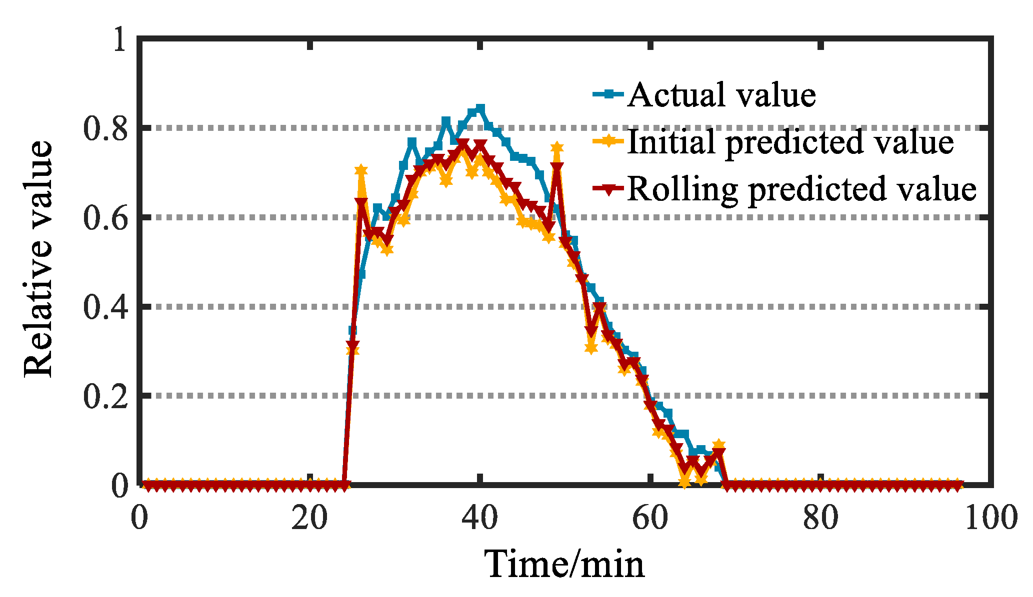Reference [9] proposes a robust model that can analyze cloud volume changes and ambient temperature (an important factor affecting PV output) to assess short-term PV output. The Rolling Forecast, by constantly updating the input conditions, can update the input data in time and correct the forecast results. Reference [10] proposes a short-term power rolling prediction model for photovoltaic power generation based on the Particle Swarm Optimization Support Vector Machine (PSO-SVM). If the forecasted power cannot satisfy the given forecast accuracy, then the actual power is used to revise the forecasted power. Reference [11] achieves a simulation of the whole year by iterating the model conditions every 24 h in a year. The model proposed in this paper can also achieve a long-term continuous operation by updating the input data.

Common methods in dealing with uncertain problems include stochastic programming [12], robust optimization [13], and IGDT. Stochastic programming usually requires the assumption that the probability distribution of random parameters is known. But robust optimization and IGDT don’t requires the assumption on the density function of uncertain parameters and instead introduce the probabilistic measure of risk [13]. The IGDT can obtain the maximum fluctuation range allowed by the uncertainty parameter while ensuring that the result is not worse than the expected target. Hence, a robust decision-making scheme can be given according to the expected cost of the decision maker. This paper studies the problem of the output of the DG under the condition of ensuring the PSC. IGDT can solve this problem very well, so this paper introduces IGDT theory into the rapid evaluation of the PSC of the ADS. IGDT is divided into Risk Averse Strategy (RAS) and Risk Seeker Strategy (RSS), which provides decision makers with more choices. Because of its strong applicability, convenient use, and high computational efficiency when dealing with parameter uncertainties, the theory has been widely used in power systems. For example, Reference [14], based on IGDT, studies the multi-source combined optimization unit commitment problem. Reference [15], based on hybrid stochastic programming and IGDT, establishes a virtual power plant scheduling optimization model. Reference [16] proposes a three-phase optimal power flow algorithm based on IGDT. Reference [17] proposes a non-probabilistic IGDT model to model the uncertainties in short-term scheduling of a generation company. The self-scheduling problem is formulated for risk-neutral, risk-averse, and risk-seeker generation company.

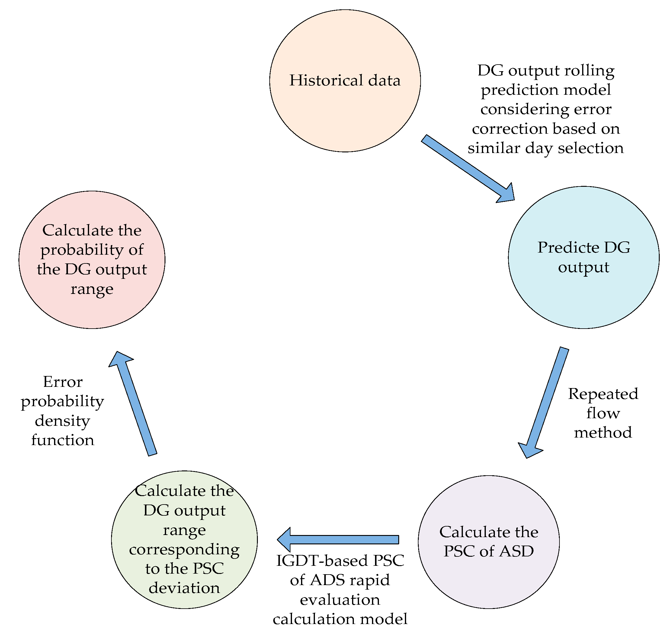
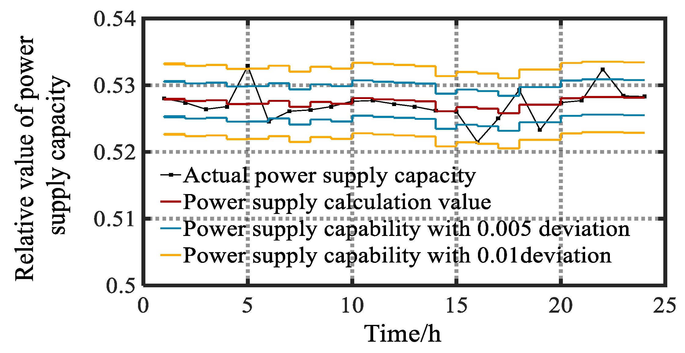
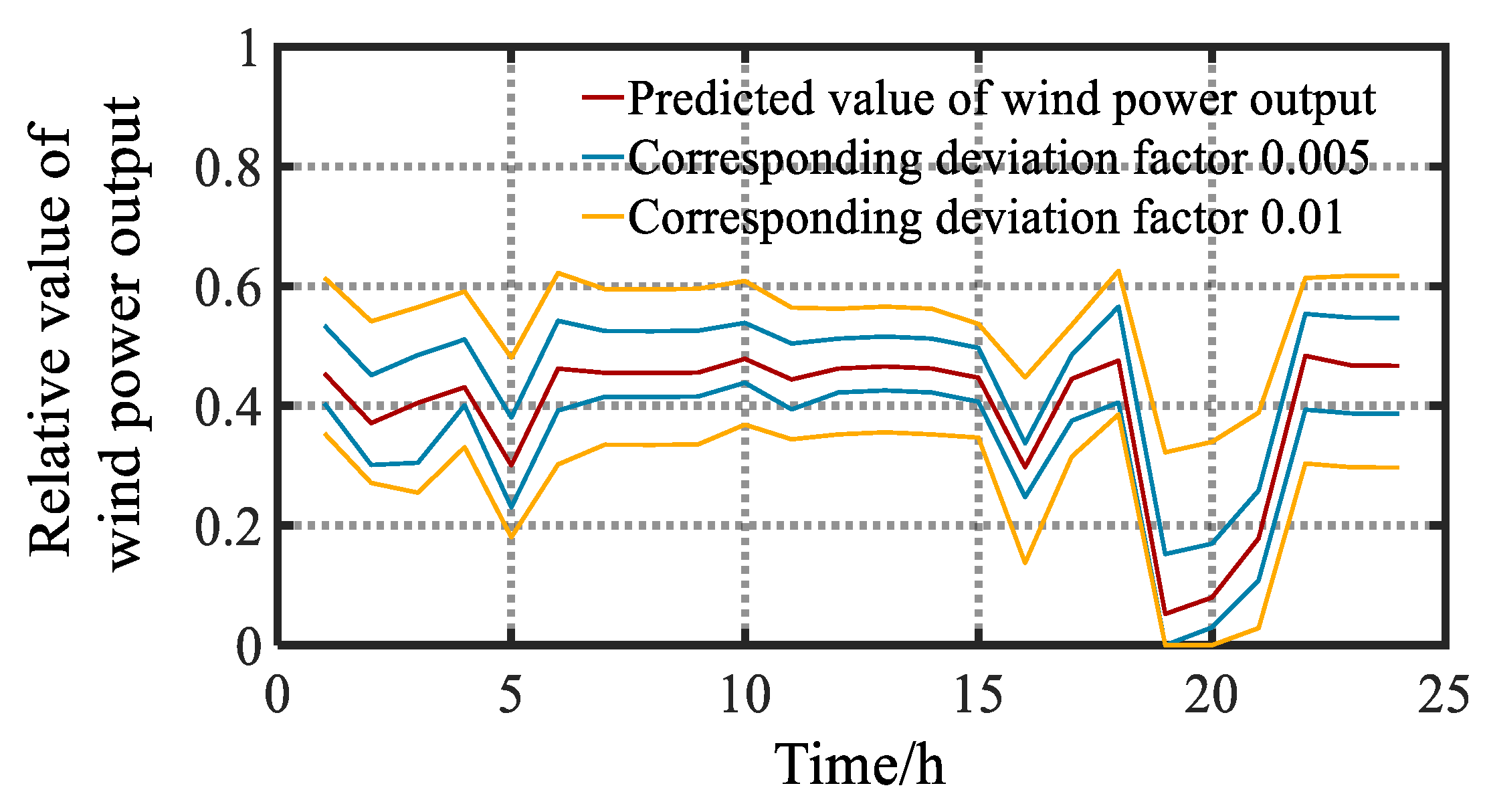
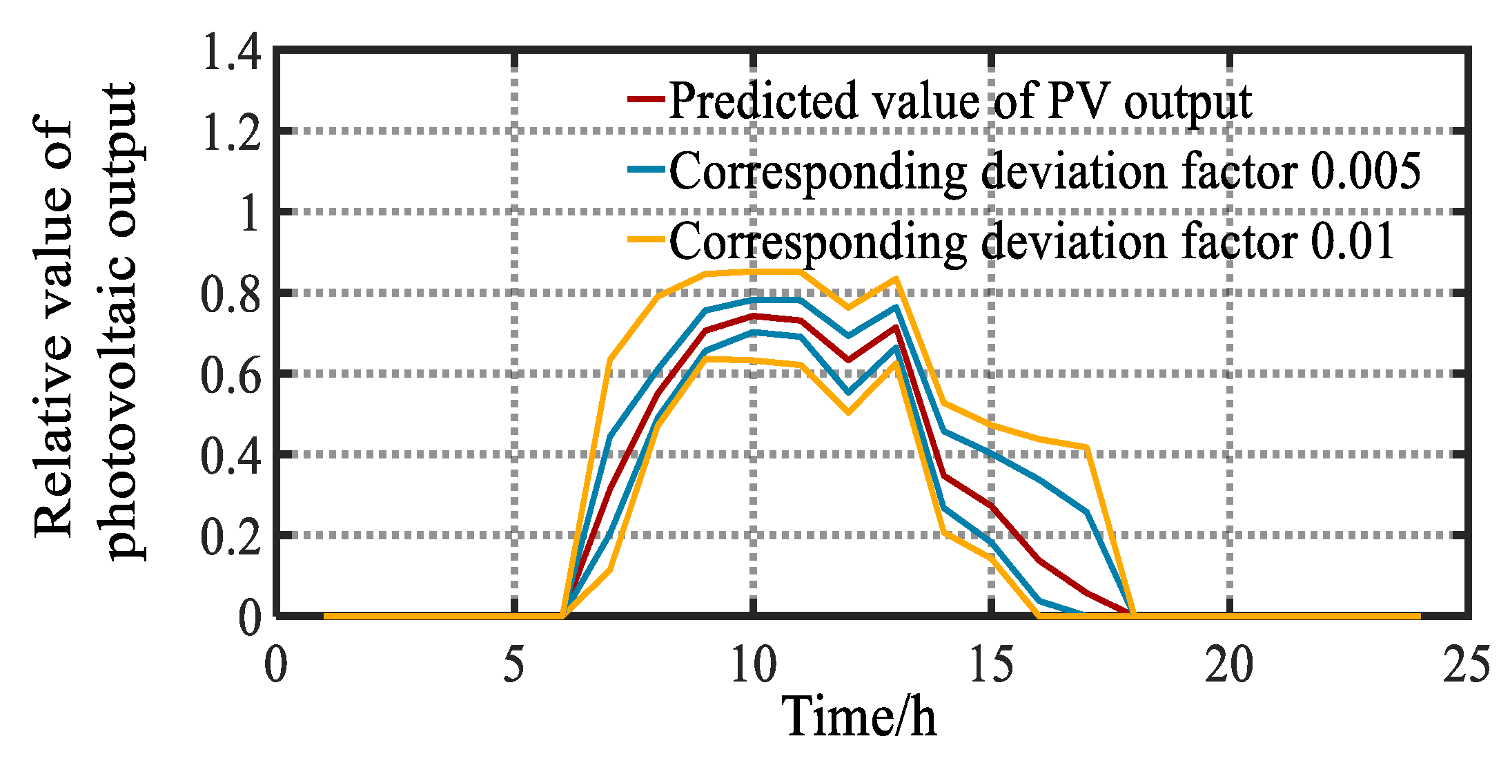
In this paper, the IGDT is introduced into the rapid evaluation of the PSC to deal with the uncertainty of the DG output, to determine the corresponding relationship between the PSC of the ADS and DG output, and then to convert the calculating probability of the PSC range into the calculating probability of the corresponding DG output range. Firstly, this paper establishes the DG output rolling prediction model based on the similar day selection error correction. The DG output prediction value is used to calculate the corresponding PSC of the ASD through the repeated power flow method. Next, this paper establishes a IGDT-based PSC of the ADS rapid evaluation calculation model to calculate the DG output range corresponding to the PSC range, and perform probability calculation. Finally, the method is verified by example. The main contributions of this paper are highlighted as follows:

• Propose a DG output rolling prediction model based on similar day selection and error correction, which provides a basis for analyzing the PSC of the ADS.
• Using IGDT theory to extract the uncertainty of DG output, and quantify the impact of DG output on PSC.

2. DG Output Rolling Prediction Model Considering Error Correction Based on Similar Day Selection

Photovoltaic output is influenced by many factors, including fixed environmental factors such as geographical location and irradiation angle and variable environmental factors such as light intensity, temperature, humidity, and cloud amount, as well as factors related to the characteristics of the self-device such as conversion efficiency [18]. By analyzing the effect of different environmental factors on the photovoltaic power generation, the light intensity and temperature data that most significantly affect the photovoltaic power generation are selected as the criteria for selecting environmental factors for similar days. First, the prediction error probability density function is established by using the similar-day prediction error. Then, the prediction error density function based on the similar day is used for sampling to obtain the prediction fitting value on the forecast date. Finally, the final forecast value is obtained after the volatility analysis is sorted. The change of wind speed is the main factor that causes the change of wind power output. Therefore, this paper first defines a method based on wind similarity to obtain similar days. The following is a brief introduction to the prediction model using photovoltaics as an example.

2.1. Selection of Photovoltaic Similar Days

By analyzing the influence of different environmental factors on the photovoltaic power generation, the light intensity and temperature data with the most obvious influence on the photovoltaic power generation are selected as the environmental factors for the similar day selection. The selected daily weather feature vector (s_i) is:

$$s_i=[thi,tli,lhi,lli]$$

(1)

where: thi is the highest temperature on i-th day; tli is the lowest temperature on i-th day; lhi is the maximum light intensity on i-th day; lli is the minimum light intensity on i-th day. The s_o represents the day to be predicted, and the similarity (Ss_im) between s_o and the i-th historical day is [19]:

$$Ssim(i)=\frac{1}{{\displaystyle \sum _{j=1}^n{\beta }_j\left|s_i(j)-s_o(j)\right|}+\epsilon }$$

(2)

where: β_j is the weight corresponding to each factor; ε is a relatively small number.

2.2. Determination of Fitting Value of DG Output Error Based on Similar Day and Error Correction

In this paper, the relative error of DG output prediction is used to describe the accuracy of wind power forecasting. The definition is shown in Equation (3).

$${\delta }_{wi}=\frac{P_{wf,i}-P_{wa,i}}{P_{wa,i}}$$

(3)

where: δ_wi is the relative error of the i-th predicted node; P_wf,i and P_wa,i are the predicted and actual values of the i-th predicted node.

Through the error statistical analysis of the prediction of historical data, it is found that the appropriate single-peak probability density function can be selected to fit the distribution of relative error. According to the theory of probability statistics, the normal distribution function has good properties and can be used to approximate many probability distributions. Therefore, the normal distribution is used to estimate the error caused by wind power output forecasting. Next, the systematic sampling method is used to sample the compensation values for 96 time points.

2.3. Predictive Compensation Value Rolling Determination Based on Volatility Analysis

2.3.1. Generation of Compensation Values for DG Power Prediction Errors Based on Volatility Analysis

By analyzing the fluctuation direction of the short-term DG power prediction error and the regularity of the amplitude, the prediction method can be used to predict the trend of the error and generate the corresponding compensation value [20].

During the fluctuation analysis, n samples from historical relative error (RE) data are applied to build up measuring standards for short-term estimation. The long-term variance is presented as ${\sigma }_l^2$ and the critical value of the absolute slope of fitting straight-line is presented as k_l:

$${\sigma }_l^2=\frac{1}{n}{{\displaystyle \sum _{i=1}^n(x_i-\frac{1}{n}{\displaystyle \sum _{i=1}^n{x}_i})}}^2$$

(4)

$$k_l=\frac{|k_1-k_2|}{4}$$

(5)

where: k₁ and k₂ are the up and down critical value of one-sided probability interval determined by simulation model and probability level, respectively.

Three RE values ahead of the forecast time are chosen to be short-term RE samples, and the calculation of the variance ${\sigma }_s^2$ as well as the absolute slope of the fitting straight-line k_s is done. The calculation results of the two variables indicate the investigation methods for RE fluctuation, which is shown in

Table 1. The investigation method of relative error (RE) fluctuation.

Value Judgment	Fluctuation	Investigation Methods
${\sigma }_s^2$ < ${\sigma }_l^2$ and ks < kl	low amplitude, steady	Moving average
${\sigma }_s^2$ < ${\sigma }_l^2$ and ks > kl	low amplitude, not steady	Auto regressive moving average
${\sigma }_s^2$ > ${\sigma }_l^2$ and ks < kl	high amplitude, steady	Weighted moving average
${\sigma }_s^2$ > ${\sigma }_l^2$ and ks > kl	high amplitude, not steady	Liner method

.

On the basis of estimated values of RE from investigation methods from Table 1, the error compensation rule is formed. The threshold δ₀ is the boundary to divide big error and small error. By comparing RE estimated values δ_i at the point i and δ_{i − 1} at point i − 1 to δ₀, respectively, the compensation methods of estimated RE would be ascertained, as in

Table 2. Compensation methods of estimated RE.

Value Judgment	Compensation Methods
δi < δ0 and δi − 1 < δ0	None
δi < δ0 and δi − 1 > δ0	1 magnitude of the estimated values
δi > δ0 and δi − 1 < δ0	1 magnitude of the estimated values
δi > δ0 and δi − 1 > δ0	1/2 magnitude of the estimated values

.

Based on fluctuation analysis, the sampling results are sequenced by compensation values. The sampling values closest to the compensation ones are elected to be the fitted values of relative error at corresponding time points, aiming to correct the forecast values of the DG output, and moreover, improve forecasting accuracy.

2.3.2. DG Output Rolling Prediction Model Based on Similar Day and Error Correction

This paper uses a historical day similar to the forecast date as a sample set of prediction error data. Then, using the volatility analysis, the closest correction value is selected as the next time correction value from the prediction error sample values, and the prediction result is corrected. The prediction method uses the Wavelet Neural Network (WNN) modified by Adaptive Dynamic Programming (ADP) correction link to predict the DG output, and uses the actual measurement data to update the WNN parameters to improve the prediction accuracy.

3. IGDT-Based PSC of ADS Rapid Evaluation Calculation Model

3.1. PSC Calculation Model

3.1.1. Objective Function

$$\max P_{\mathrm{L}}={\displaystyle \sum _{i=1}^N{P}_{\mathrm{L}i}}$$

(6)

where: P_L is the maximum active load that the distribution network can supply; N is the number of load points; P_Li is the active load at load point i.

3.1.2. Constraints

$$P_{\mathrm{G}i}+P_{\mathrm{DG}i}-P_{\mathrm{L}i}=U_i{\displaystyle \sum _{j=1}^N{U}_j(G_{ij}\cos {\theta }_{ij}+B_{ij}\sin {\theta }_{ij})}$$

(7)

$$Q_{\mathrm{G}i}+Q_{\mathrm{DER}i}-Q_{\mathrm{L}i}=U_i{\displaystyle \sum _{j=1}^N{U}_j(G_{ij}\cos {\theta }_{ij}-B_{ij}\sin {\theta }_{ij})}$$

(8)

$$U_i^{\min }\le U_i\le U_i^{\max }$$

(9)

$$I_l\le I_l^{\max }$$

(10)

where: P_Gi, P_DGi and P_Li are the active power of the generator, DG, and load at node i; Q_Gi, Q_DGi and Q_Li are the reactive power of the generator, DG and load at node i; G_ij and B_ij are conductance and susceptance of the branch i-j; θ_ij is the power angle between the node i and the node j; U_i, $U_i^{\max }$ and $U_I^{\min }$ are the voltage at the node i and its upper and lower limits; I_l and $I_l^{\max }$ are respectively the line l Current and its upper limit.

When the traditional PSC calculation model calculates the objective function value, it needs to determine both the active and reactive power at each node, and then solves the solution under the constraint condition through a certain calculation method. Therefore, the traditional calculation model cannot take into account the uncertainty of the DG output. For this reason, this paper introduces IGDT theory into the calculation model of the PSC, and deduce the uncertainty of the DG.

3.2. The Basic Theory of IGDT

IGDT is a mathematical optimization method for models with uncertain parameters [21]. Its role is to study the possible effects of uncertain parameters on the premise of meeting the preset targets. According to the preset goals, its impact can be divided into negative and positive. The corresponding models are called risk avoidance model (RAM) and risk speculation model (RSM). They correspond to two diametrically opposed values adopted by decision makers in the face of risk: One, considers that the existence of uncertain parameters will have a negative impact on the target expectations, and the other considers uncertain parameters to be favorable [22].

Consider the following optimization model:

$$\{\begin{array}{l}\min B(X,d)\hfill \\ \begin{array}{r}\hfill \begin{array}{cc}s.t.& H(X,d)=0\end{array}\\ \hfill G(X,d)\ge 0\end{array}\hfill \end{array}$$

(11)

where: X is an uncertain parameter; d is a decision variable; B(X,d) is an objective function; H(X,d), G(X,d) are equality and inequality constraints.

In IGDT theory, the uncertainty of the parameter X around the predicted value $\tilde{X}$ can be described as follows:

$$\{\begin{array}{c}X\in U(\alpha ,\tilde{X})\hfill \\ U(\alpha ,\tilde{X})=\left\{X:\left|\frac{X-\tilde{X}}{\tilde{X}}\right|\le \alpha \right\}\hfill \end{array}$$

(12)

where: α represents the fluctuation amplitude of uncertain parameters, α ≥ 0; $U(\alpha ,\tilde{X})$ means that the range of uncertainty parameter X deviating from the predicted value does not exceed $\mathsf{\alpha }\left|\tilde{X}\right|$.

In an uncertain environment, conservative decision makers usually maximize the unfavorable disturbances of uncertain parameters in order to ensure the achievement of a low-expectation goal. The aggressive decision-makers are more likely to seek the additional benefits of uncertainty. The mathematical model corresponding to the two strategies is as follows:

$$\{\begin{array}{cc}\max \alpha \hfill & \\ s.t.\hfill & \underset{X}{\max } B(X,d)\le B_c\\ & B_c=(1+{\beta }_c)B_0\\ & \forall X\in U(\alpha ,\tilde{X})\\ & H(X,d)=0\\ & G(X,d)\ge 0\end{array}$$

(13)

$$\{\begin{array}{cc}\min \alpha \hfill & \\ s.t.\hfill & \underset{X}{\min } B(X,d)\le B_O\\ & B_O=(1+{\beta }_O)B_0\\ & \forall X\in U(\alpha ,\tilde{X})\\ & H(X,d)=0\\ & G(X,d)\ge 0\end{array}$$

(14)

where: B₀ is the objective function value when X is taken as $\tilde{X}$; β_c, β_o are deviation factors, which represent the degree of deviation of expected cost above or below B₀; for a given d, maxB(X,d) and minB(X,d) are functions of X. If the two changes with X can be explicitly determined, their concrete expression can be intuitively represented.

Equation (13) is a RAM, which means that the decision value d obtained under the model can guarantee that the expected cost is not higher than B_c for any disturbance $X\in U(\alpha ,\tilde{X})$. Equation (14) is a RSM, which means that for the decision value d obtained under this model, there is at least one $X\in U(\alpha ,\tilde{X})$, so that the expected cost is not higher than B_o.

3.3. Application of IGDT in Power Supply Capacity Calculation Model

In this paper, maxP_L is used as the objective function and P_DGi is set as the uncertainty parameter. That is, corresponding to different deviation factors β_c and β_o, according to Equations (13) and (14), the corresponding P_DGi fluctuation amplitude α can be solved. According to Equation (12), the DG output fluctuation range can be expressed as:

$$U({\alpha }_{w,t},{\tilde{P}}_{w,t})=\left\{P_{w,t}:(1-{\alpha }_{w,t}){\tilde{P}}_{w,t}\le P_{w,t}\le (1+{\alpha }_{w,t}){\tilde{P}}_{w,t}\right\}$$

(15)

$$U({\alpha }_{s,t},{\tilde{P}}_{s,t})=\left\{P_{s,t}:(1-{\alpha }_{s,t}){\tilde{P}}_{s,t}\le P_{s,t}\le (1+{\alpha }_{s,t}){\tilde{P}}_{s,t}\right\}$$

(16)

where: ${\tilde{P}}_{w,t}$ and ${\tilde{P}}_{s,t}$ are predicted values of wind farm and photovoltaic field output; ${\alpha }_{w,t}$ and ${\alpha }_{s,t}$ are corresponding fluctuation amplitudes, and their values are directly related to prediction error.

3.3.1. RAM for PSC Prediction

When the DG output is lower than the predicted value, the distribution network needs to transmit more power from the upper-level power grid, which will inevitably lead to a decrease in the maximum PSC of ADS. Therefore, in the RAM, in order to ensure that the PSC of the ADS is not lower than a certain lower limit, the DG output is calculated according to the following formula:

$$P_{w,t}=(1-{\alpha }_{w,t}^c){\tilde{P}}_{w,t},t\in T,w\in W$$

(17)

$$P_{s,t}=(1-{\alpha }_{s,t}^c){\tilde{P}}_{s,t},t\in T,s\in S$$

(18)

Since the objective function of this paper is the PSC, it is hoped that the PSC is as large as possible, and the IGDT theoretical objective function is the cost, and the smaller the cost, the better. Therefore, in the calculation process, the objective function is calculated as follows:

$$f=-\max P_L$$

(19)

where: f is equivalent to parameter B in IGDT theory, so the calculation of f₀ is similar to the calculation of B₀. f₀ is the negative value of the maximum PSC of the ADS when the DG output takes the predicted value. Under the RAM, the maximum value of the objective function should not be higher than $(1+{\beta }_c)f_0,{\beta }_c\le 0$.

Because IGDT has a single uncertainty coefficient of deviation as the objective function, it cannot be applied to the simultaneous processing of wind power and photovoltaic output uncertainty. This paper solves the above problems by giving different weights to the wind force output deviation coefficient.

$$k_{w,t}\alpha ={\alpha }_{w,t}^c$$

(20)

$$k_{s,t}\alpha ={\alpha }_{s,t}^c$$

(21)

$$k_{w,t}+k_{s,t}=1,t\in T,w\in W,s\in S$$

(22)

where: ${\alpha }_{w,t}^c$ and ${\alpha }_{s,t}^c$ are the deviation coefficients of wind power and photovoltaic output respectively; k_w,t and k_s,t are the weights of the deviation coefficients, and their effects are the guiding model to obtain the alpha value that matches the actual error, so that the scheduling scheme is more reasonable and reliable. The greater the DG output, the greater the impact on the PSC of the ADS, hence, the weight coefficient is calculated according to the following formula:

$$k_{w,t}=\frac{{\tilde{P}}_{w,t}}{{\displaystyle \sum _{w\in W}{\tilde{P}}_{w,t}}+{\displaystyle \sum _{s\in S}{\tilde{P}}_{s,t}}},t\in T,w\in W,s\in S$$

(23)

Finally, the RAM that considers the uncertainty of DG output is as follows:

$$\{\begin{array}{ll}\max \alpha \hfill & \\ s.t.\hfill & (2)-(5)\hfill \\ & f\le (1+{\beta }_c)f_0\hfill \\ & P_{w,t}=(1-{\alpha }_{w,t}^c){\tilde{P}}_{w,t}\hfill \\ & P_{s,t}=(1-{\alpha }_{s,t}^c){\tilde{P}}_{s,t}\hfill \\ & {\alpha }_w^c\ge 0,{\alpha }_s^c\ge 0\hfill \end{array}$$

(24)

3.3.2. RSM for PSC Prediction

In the RSM, the decision makers are optimistic about the volatility of the DG output. Therefore, it can be considered that when the DG output is higher than the predicted output, the PSC of the ADS can be increased. Therefore, in the RSM, in order to ensure that the PSC of ADS may be higher than a certain upper limit, the DG output is calculated according to the following formula:

$$P_{w,t}=(1+{\alpha }_{w,t}^c){\tilde{P}}_{w,t},t\in T,w\in W$$

(25)

$$P_{s,t}=(1+{\alpha }_{s,t}^c){\tilde{P}}_{s,t},t\in T,s\in S$$

(26)

In the same way, the final RSM can be derived as:

$$\{\begin{array}{ll}\min \alpha \hfill & \\ s.t.\hfill & (2)-(5)\hfill \\ & f\le (1-{\beta }_o)f_0\hfill \\ & P_{w,t}=(1+{\alpha }_{w,t}^o){\tilde{P}}_{w,t}\hfill \\ & P_{s,t}=(1+{\alpha }_{s,t}^o){\tilde{P}}_{s,t}\hfill \\ & {\alpha }_w^o\ge 0,{\alpha }_s^o\ge 0\hfill \end{array}$$

(27)

3.4. DG Output Range Probability Calculation

The confidence interval estimation can quantify the change of the prediction result caused by the uncertainty factor, so that the actual observation value falls within the prediction interval corresponding to a certain confidence level. It can provide more information to decision makers and help them better understand the uncertainties and risks that may exist when the predicted value changes in the future.

Therefore, this paper uses the confidence interval estimation method to calculate the confidence of the predicted output in this interval after solving the wind power and PV output range, so as to quantify the results and provide more specific and powerful information for decision makers. The specific steps are as follows:

After obtaining the DG output range by IGDT-based PSC of the ADS rapid evaluation calculation model, this paper calculates the probability of the DG output range based on the DG output prediction error probability density function. The specific steps are as follows:

• Using the statistics of similar daily prediction errors performed in the prediction part, the prediction error probability density function is established;
• Calculate the fluctuation range of the DG output corresponding to the corresponding deviation factor by solving the IGDT model;
• Calculate the probability of the corresponding wind power and PV fluctuation amplitude. The weighted sum is the probability corresponding to the DG output range, that is, the probability of corresponding PSC deviation. Figure 1 shows the prediction error probability density function of wind power.

4. Model Solving

By definition, the PSC of the ADS is equal to the total load supplied by the distribution network when a certain constraint condition is not met in the model. The most direct method is the repeat power flow method. The basic idea is: From the current operating point, according to a certain load growth mode, the system load is continuously increased and the power flow calculation is repeated to determine the system PSC [23]. In this paper, the variable step is used to solve the problem [24]. The particle swarm optimization algorithm was inspired by Eberhart and Kennedy in simulating a simplified social model. The idea stems from the organization of social behavior and the search for optimal solutions through inter-individual collaboration. The traditional particle swarm optimization algorithm can be found in the literature [25,26]. In solving the PSC model of distribution network based on IGDT, this paper uses the improved particle swarm optimization algorithm to solve the problem. The calculation process is as follows:

• DG output prediction. Based on historical data, rolling forecast for photo voltaic and wind power output.
• Calculation of PSC. Based on the predicted value of the DG output, the PSC value is calculated.
• Set the deviation factors β_c and β_o, and calculate the fluctuation range of the DG output. When the PSC deviation is 0.005 and 0.01, the total deviation range of the DG output and the corresponding wind power and photo voltaic deviation range are calculated respectively by using the particle swarm optimization algorithm. The algorithm first generates a random solution about the fluctuation range of DG output; secondly, it calculates the corresponding deviation factor, and takes the difference between the corresponding deviation factor and the set deviation factor as the fitness function of the particle; thirdly, it finds the optimal solution and then proceeds to the next iteration. When the difference between the optimal deviation factor and the set deviation factor is less than the set value, the loop ends.
• Calculation of the probability of the DG output range. After solving the DG output fluctuation range, the probability of wind power and PV in the corresponding interval is calculated to provide more specific and powerful information for decision makers. The flow chart is shown in Figure 2.

5. Case Analysis

5.1. Parameters of Case

In order to verify the feasibility and effectiveness of the proposed model, this paper selects the historical output data and meteorological data of a wind farm and a photovoltaic power station for verification. Then the improved IEEE-14 node system is used for PSC evaluation. MATLAB is used for simulation calculation. Considering that the distribution network is normally operated in open-loop condition, this paper removes the three branches of 14, 15, and 16 to make the system a single-supply radiating network with 14 nodes and 13 branches. The structure is shown in Figure 3.

In Figure 3, node 1 is the balance node, and the rest are load nodes. The system reference capacity is 100 MVA and the reference voltage is 23 kV. The thermal stability limit capacity is the upper limit of line power and the allowable range of voltage is 1 ± 5%.

In addition to the fixed load, the DG of the connected distribution network includes: Wind power (WG) and photo voltaic (PV). The access conditions are shown in

Table 3. Connections of the “Units” of ADS.

Access Node	Access Capacity/kW	Access Type
2	500	WG
3	300	PV
4	300	PV
8	500	WG

.

5.2. Result of Calculation Example

5.2.1. DG Output Prediction

According to the rolling prediction method, the predicted result is corrected by rolling correction. The actual value, initial predicted value, and rolling predicted value are compared and the comparison results are shown in Figure 4 and Figure 5.

As can be seen from Figure 4 and Figure 5, the rolling prediction result is closer to the actual DG output value. In order to quantify the effect of the prediction, the root mean square error (RMSE), the mean absolute error (MAE), the mean absolute percentage error (MAPE), and the maximum relative error (ME) are respectively calculated for the direct prediction result and the error compensated prediction result [27]. The calculation formula of the indicator is:

$$MAE={\displaystyle \sum _{t=1}^n(Y_t-y_t)/n}$$

(28)

$$RMSE=[{\displaystyle \sum _{t=1}^n{(Y_t-y_t)}^2/n{]}^{1/2}}$$

(29)

$$MAPE={\displaystyle \sum _{t=1}^n(\frac{\left|Y_t-y_t\right|}{y_t})}/n\times 100\%$$

(30)

$$ME=\max (Y_t-y_t)$$

(31)

where: Y_t is the predicted value; y_t is the actual value; n is the number of predicted points. The data is shown in

Table 4. Comparison of prediction error before and after compensation of wind power output.

Type	MAE	RMSE	MAPE/%	ME
Initial prediction error	0.0429	0.0626	18.937	0.1869
Prediction error after compensation	0.0376	0.0547	14.033	0.1789

and

Table 5. Comparison of prediction error before and after compensation of PV.

Type	MAE	RMSE	MAPE/%	ME
Initial prediction error	0.1227	0.1626	14.547	0.0943
Prediction error after compensation	0.1042	0.1313	9.247	0.0879

.

Based on Figure 4 and Figure 5, and Table 4 and Table 5, it can be seen that the sampling value of relative error fit distribution can effectively eliminate the extreme values appearing in the volatility analysis, the error divergence and over-compensation phenomenon can also be avoided. The volatility analysis has the ability to initially estimate the compensation value of the relative error. Based on the sampling error, the DG output prediction value can be accurately matched with the fitting relative error value, thereby achieving the compensation of the error and improving the prediction accuracy.

5.2.2. PSC Calculation

According to the predicted value of DG output, the prediction value of the 24-h PSC of ASD is calculated. And the PSC value of corresponding to actual DG output is as shown in

Table 6. PSC comparison.

Time	Predicted PSC	Actual PSC	Time	Predicted PSC	Actual PSC
1	0.5279	0.5280	13	0.5277	0.5268
2	0.5278	0.5274	14	0.5275	0.5262
3	0.5276	0.5264	15	0.5261	0.5260
4	0.5277	0.5268	16	0.5267	0.5215
5	0.5271	0.5349	17	0.5264	0.5250
6	0.5272	0.5246	18	0.5250	0.5293
7	0.5276	0.5261	19	0.5270	0.5233
8	0.5267	0.5263	20	0.5270	0.5274
9	0.5274	0.5268	21	0.5280	0.5277
10	0.5272	0.5276	22	0.5282	0.5324
11	0.5280	0.5277	23	0.5282	0.5284
12	0.5278	0.5272	24	0.5281	0.5283

and Figure 6.

In the table, the “Actual PSC” is calculated according to the actual DG output. The “Predicted PSC” is calculated according to the predicted DG output. In order to better show the relationship between the actual PSC and the predicted PSC, the actual PSC and the corresponding deviation range are compared with the predicted PSC, as shown in Figure 6.

It can be seen from Figure 6 that the predicted value of the PSC at most moments is within the range of deviation 0.005 of the actual PSC, indicating the feasibility of the PSC prediction method provided in this paper. In 5.2.3, the probability of the deviation range is further calculated and verified.

5.2.3. Probability Calculation of PSC Range and Verification

It can be seen from Figure 6 that the predicted PSC result is close to the actual PSC result, and the predicted PSC result is mainly concentrated within the range with deviation of 0.005. According to the predicted PSC value, the wind power and photo voltaic fluctuation range that meets the PSC deviation range are calculated. The calculation results are shown in Figure 7 and Figure 8.

From Figure 7 and Figure 8, the predicted value and the deviation range of the DG output at each time can be obtained. According to the model of this paper, when the DG output meets a certain deviation range, the corresponding PSC must also meet the corresponding deviation range. Therefore, the probability calculation of the PSC deviation range can be converted into the probability calculation of the corresponding DG output range. According to the calculated wind power and photo voltaic output range and the probability calculation method of this paper, the probability and actual situation corresponding to the 24-h DG output are shown in

Table 7. Probability and actual situation of power supply capability range.

Time	Probability with 0.005 Deviation	Whether the Actual PSC is Satisfied	Probability with 0.01 Deviation	Whether the Actual PSC is Satisfied
1	0.3815	yes	0.7406	yes
2	0.3127	yes	0.6013	yes
3	0.3332	yes	0.6298	yes
4	0.3278	yes	0.6247	yes
5	0.3958	no	0.7665	no
6	0.3258	no	0.6371	yes
7	0.3957	yes	0.7685	yes
8	0.3800	yes	0.7342	yes
9	0.3422	yes	0.6416	yes
10	0.3692	yes	0.6759	yes
11	0.3656	yes	0.6736	yes
12	0.3849	yes	0.7934	yes
13	0.3679	yes	0.7058	yes
14	0.3743	yes	0.7392	yes
15	0.3655	yes	0.7171	yes
16	0.3706	no	0.7532	yes
17	0.3277	yes	0.6146	yes
18	0.3397	no	0.6223	yes
19	0.3250	no	0.6317	yes
20	0.3695	yes	0.6834	yes
21	0.3439	yes	0.6682	yes
22	0.3766	no	0.7095	yes
23	0.3187	yes	0.6190	yes
24	0.3346	yes	0.6646	yes
Total/average	0.3695	18/24	0.6840	23/24

.

According to the final result, it is found that the probability of the actual PSC which satisfies the predicted deviation range is greater than the calculated result. The calculation result of this model is the weighted sum of the probabilities of wind power and photovoltaic output range. However, in actual operation, when there is wind power or photovoltaic output exceeding the calculation range, the combined result may also make the PSC meet the deviation requirement. Therefore, the calculation result of the PSC range probability is conservative, which is smaller than the actual probability. However, when the deviation reaches 0.01, the probability value is larger, and the prediction model has higher precision. Therefore, this model has certain guiding significance for the parties in the spot market transaction to master the information of the PSC.

6. Conclusions

According to the method proposed in this paper, the PSC of the ASD can be quickly calculated, and the conservative probability of PSC fluctuation within a certain range is given, which provides necessary guidance information for the spot market parties.

References

1. National Energy Administration. Available online: http://www.nea.gov.cn/2018-08/02/c_137363846.htm (accessed on 1 June 2019).
2. Zhao, H.; Yang, Q.; Zeng, H. Multi-loop virtual synchronous generator control of inverter-based DGs under microgrid dynamics. IET Gener. Transm. Distrib. 2017, 11, 795–803. [Google Scholar] [CrossRef]
3. Yu, W.; Liu, D.; Huang, Y. Operation Optimization Based on the Power Supply and Storage Capacity of an Active Distribution Network. Energies 2013, 6, 6423–6438. [Google Scholar] [CrossRef] [Green Version]
4. Miu, K.; Chiang, H. Electric distribution system load capability: Problem formulation, solution algorithm, and numerical results. IEEE Trans. Power Deliv. 2000, 15, 436–442. [Google Scholar]
5. Yang, Q.; Jiang, L.; Hao, W.; Zhou, B.; Yang, P. PMU placement in electric transmission networks for reliable state estimation against false data injection attacks. IEEE Internet Things J. Spec. Secur. Priv. Cyber Phys. Syst. 2017, 4, 1978–1986. [Google Scholar] [CrossRef]
6. Zhou, W.; Sun, K.; Sun, H.; Ma, Q.; Liu, J.; Wang, R.; Sun, J.; Jiang, X.; Chen, X. Bi-level optimization model for load supplying capability in active distribution network based on chance-constrained programming. Power Syst. Prot. Control 2018, 46, 70–77. [Google Scholar]
7. Ge, S.; Sun, H.; Liu, H.; Zhang, Q. Power Supply Capability Evaluation of Active Distribution Network Considering Reliability and Post-fault Load Response. Autom. Electr. Power Syst. 2019, 43, 77–84. [Google Scholar]
8. Shan, Y.; Fu, Q.; Geng, X.; Zhu, C. Combined Forecasting of Photovoltaic Power Generation in Microgrid Based on the Improved BP-SVM-ELM and SOM-LSF with Particlization. Proc. CSEE 2016, 12, 3334–3342. [Google Scholar]
9. Gandoman, F.H.; Aleem, S.H.A.; Omar, N.; Ahmadi, A.; Alenezi, F.Q. Short-term Solar Power Forecasting Considering Cloud Coverage and Ambient Temperature Variation Effects. Renew. Energy 2018, 123, 793–805. [Google Scholar] [CrossRef]
10. Wang, J.; Song, Z.; Ran, R. Short-term Photovoltaic Power Generation Rolling Forecast Based on Optimized SVM. Proc. CSU-EPSA 2016, 28, 9–13. [Google Scholar]
11. Bashir, A.A.; Pourakbari-Kasmaei, M.; Contreras, J.; Lehtonen, M. A novel energy scheduling framework for reliable and economic operation of islanded and grid-connected microgrids. Electr. Power Syst. Res. 2019, 171, 85–96. [Google Scholar] [CrossRef]
12. Home-Ortiz, J.M.; Pourakbari-Kasmaei, M.; Lehtonen, M.; Mantovani, J.R.S. Optimal location-allocation of storage devices and renewable-based DG in distribution systems. Electr. Power Syst. Res. 2019, 172, 11–21. [Google Scholar] [CrossRef]
13. Kazemi, M.; Mohammadi-Ivatloo, B.; Ehsan, M. Risk-based bidding of large electric utilities using Information Gap Decision Theory considering demand response. Electr. Power Syst. Res. 2014, 114, 86–92. [Google Scholar] [CrossRef]
14. Wang, C.; Wei, H.; Wu, S. Multi-power Combined Unit Commitment Based on Information Gap Decision Theory. Proc. CSEE 2017, 41, 1–9. [Google Scholar]
15. Sun, G.; Zhou, Y.; Wei, Z.; Geng, T.; Wang, Y.; Li, Y. Dispatch optimization model of virtual power plant based on hybrid stochastic programming and information gap decision theory. Electr. Power Autom. Equip. 2017, 37, 112–118. [Google Scholar]
16. Connell, A.O.; Soroudi, A.; Keane, A. Distribution Network Operation under Uncertainty Using Information Gap Decision Theory. IEEE Trans. Smart Grid 2018, 9, 1848–1858. [Google Scholar] [CrossRef]
17. Zareipour, H.; Mohammadi-Ivatloo, B.; Amjady, N.; Ehsan, M. Application of information-gap decision theory to risk-constrained self-scheduling of GenCos. IEEE Trans. Power Syst. 2013, 28, 1093–1102. [Google Scholar]
18. Gao, Y.; Yang, W.; Zhu, J.; Ren, J.; Li, P. Evaluating the Effect of Distributed Generation on Power Supply Capacity in Active Distribution System Based on Sensitivity Analysis. Energies 2017, 10, 1473. [Google Scholar] [CrossRef]
19. Gao, Y.; Sun, Y.; Yang, W.; Chuai, B.; Liang, H.; Li, P. Weather-Sensitive Load’s Short-Term Forecasting Research Based on New Human Body Amenity Indicator. Proc. CSEE 2017, 37, 1946–1955. [Google Scholar]
20. Gao, Y.; Cheng, H.; Zhu, J.; Liang, H.; Li, P. The Optimal Dispatch of a Power System Containing Virtual Power Plants under Fog and Haze Weather. Sustainability 2016, 8, 71. [Google Scholar] [CrossRef]
21. Haim, Y.B. Info-Gap Decision Theory; Academic Press: San Diego, CA, USA, 2006; pp. 267–296. [Google Scholar]
22. Song, K.; Xie, Y.; Chen, X.; Zhang, L. Robust Restoration Method for Power System Load Based on Information Gap Decision Theory. Autom. Electr. Power Syst. 2017, 41, 113–120. [Google Scholar]
23. Cornélusse, B.; Vangulick, D.; Glavic, M.; Ernst, D. Global capacity announcement of electrical distribution systems: A pragmatic approach. Sustain. Energy Grids Netw. 2015, 4, 43–53. [Google Scholar] [CrossRef] [Green Version]
24. Guo, Z.; Wei, G.; Li, M.; Chu, J.Y. Assessment of Power Supply Capability for Distribution Network with Distributed Generations. Mod. Electr. Power 2015, 32, 56–61. [Google Scholar]
25. Yin, Z.; Xiao, L.; Sun, X.; Liu, J.; Zhong, Y. A speed estimation method of fuzzy extended kalman filter for induction motors based on particle swarm optimization. Trans. China Electrotech. Soc. 2016, 31, 55–65. [Google Scholar]
26. Tavakkoli, M.; Adabi, J.; Zabihi, S.; Godina, R.; Pouresmaeil, E. Reserve Allocation of Photovoltaic Systems to Improve Frequency Stability in Hybrid Power Systems. Energies 2018, 11, 2583. [Google Scholar] [CrossRef]
27. Wu, X.; Chen, F. Prediction Methods for Nonparametric Regression Models with Fixed Design and Heteroscedasticity. Stat. Decis. 2017, 17, 76–79. [Google Scholar]
Figure 1. Prediction error probability density function of wind power.
Energies 12 02223 g001
Figure 2. Flow chart.
Energies 12 02223 g002
Figure 3. Improved IEEE14 node figure.
Energies 12 02223 g003
Figure 4. Comparison of wind power prediction results.
Energies 12 02223 g004
Figure 5. Comparison of PV prediction results.
Energies 12 02223 g005
Figure 6. Power supply solution results.
Energies 12 02223 g006
Figure 7. Wind power output range.
Energies 12 02223 g007
Figure 8. Photo voltaic output range.
Energies 12 02223 g008