Article

HVAC Optimization Genetic Algorithm for Industrial Near-Zero-Energy Building Demand Response

by
Nikolaos Kampelis
1,*,
Nikolaos Sifakis
2,
Dionysia Kolokotsa
1,
Konstantinos Gobakis
1,
Konstantinos Kalaitzakis
3,
Daniela Isidori
4 and
Cristina Cristalli
4
1
Energy Management in the Built Environment Research Lab, School of Environmental Engineering, Technical University of Crete, Technical University Campus, Kounoupidiana, GR 73100 Chania, Greece
2
Renewable and Sustainable Energy Systems Laboratory, School of Environmental Engineering, Technical University of Crete, Kounoupidiana, GR 73100 Chania, Greece
3
Electric Circuits and Renewable Energy Sources Laboratory, Technical University of Crete; Kounoupidiana, GR 73100 Chania, Greece
4
Research for Innovation, AEA srl, Angeli di Rosora, 60030 Marche, Italy
*
Author to whom correspondence should be addressed.
Energies 2019, 12(11), 2177; https://doi.org/10.3390/en12112177
Submission received: 30 April 2019 / Revised: 3 June 2019 / Accepted: 4 June 2019 / Published: 7 June 2019
(This article belongs to the Special Issue Intelligent Control in Energy Systems Ⅱ)

Abstract

:
Demand response offers the possibility of altering the profile of power consumption of individual buildings or building districts, i.e., microgrids, for economic return. There is significant potential of demand response in enabling flexibility via advanced grid management options, allowing higher renewable energy penetration and efficient exploitation of resources. Demand response and distributed energy resource dynamic management are gradually gaining importance as valuable assets for managing peak loads, grid balance, renewable energy source intermittency, and energy losses. In this paper, the potential for operational optimization of a heating, ventilation, and air conditioning (HVAC) system in a smart near-zero-energy industrial building is investigated with the aid of a genetic algorithm. The analysis involves a validated building energy model, a model of energy cost, and an optimization model for establishing HVAC optimum temperature set points. Optimization aims at establishing the trade-off between the minimum daily cost of energy and thermal comfort. Predicted mean vote is integrated in the objective function to ensure thermal comfort requirements are met.

1. Introduction

Demand response (DR) refers to ways of altering the power consumption of buildings, settlements, or other facilities, within a specific time frame, for economic return [1]. It implies regulatory, technological, and market changes affecting the way energy is transacted and exploited. Demand response is strongly interlinked with the smart grid technological paradigm. By definition, consumers are able to adjust their power purchasing patterns according to dynamic exchange of information, incentives, and disincentives [2]. Demand response is linked to sustainable development goal (SDG) 7 for ensuring access to affordable, reliable, sustainable, and modern energy for all [3]. DR is directly linked to targets for increasing the share of renewables and improving energy efficiency in smart grids. Wide implementation of DR is expected to be complementary to SDG 13 as part of the efforts to keep global warming to well below 2 °C above pre-industrial levels.
Distributed energy resources (DER) and demand response (DR) are gradually gaining ground in this context with respect to (a) the reduction of peak loads, (b) maintaining grid balance, and (c) dealing with the volatility of renewable energy sources (RES). Maintaining grid balance is a prerequisite for the provision of high-quality power utility services affecting everyday life, as well as social and economic progress.
According to Reference [4], demand-side management (DSM) measures can be categorized based on the timing and the impact of the measure into energy efficiency, time of use, demand response, and spinning reserve. Demand response is further classified into (i) incentive-based, including direct load control, interruptible/curtailable rates, emergency DR, capacity market programs, and demand bidding programs, and (ii) time-based, such as time of use (ToU) rates, critical peak pricing (CPP), and real-time pricing (RTP). In RTP, end customers are forwarded wholesale market prices a day or an hour before energy delivery. The main challenge in RTP is associated with the requirement for robust and continuous real-time communication between the energy provider and customers [5]. Prices in RTP fluctuate as a consequence of wholesale market price variation and design aspects. Several RTP structures were assessed by utilities [5].
In this framework, the idea of an open and transparent smart grid accommodating participants on a fair and inclusive basis is tied with (a) the allocation of actual costs for the generation, transmission, and distribution to the various stakeholders, and (b) the transition to a very high share of clean energy resources in the electricity generation mix. Undoubtedly, the smart grid of the next decade needs to ensure very high penetration of RES, as well as gradual replacement of fossil fuels and other power sources associated with high environmental risks. Grid energy efficiency is currently related, among others, to requirements for significant levels of spinning reserves and low-efficiency generators compromising environmental sustainability. In DR, consumers are incentivized to control their consumption in time to follow high RES production, contribute to the decrease of demand peaks, and lead to an improved overall energy efficiency at grid level.
The potential benefits of DR for customers, system operation, market efficiency, and reliability of the power system were critically evaluated based on different innovative technologies, real case studies, and research projects [2,6,7].
On the contrary, there are several factors slowing down the widespread implementation of DR as reported by various authors reflecting various human intrinsic, economic, social, technological, and regulatory aspects, as discussed in References [8,9,10]. In terms of the infrastructure modernization necessary for DR to take place, smart meters and advanced metering infrastructure (AMI) have a fundamental role to play. Advanced metering infrastructure, such as smart meters, is an essential part of the smart grid for utilities to be able to monitor and control any point of energy consumption/production or distribution in the grid. AMI and smart meters are also essential for consumers to be able to monitor their consumption and react to information about prices or DR events in real time. Various forms of possible DR program types and interactions between stakeholders involved such as utilities, aggregators, and resources are defined in the Open ADR standard [11].
Adding flexibility in power consumption provides a sound basis for improving the grid’s environmental performance. Reduction of peak loads at grid level could lead to a lower level of operation for generation plants of high running cost, low efficiency, and low environmental performance. DR potential in the United States (US) alone could lead to peak load reductions of 150 GW, an equivalent of approximately 2000 peaking plants [12].
A thorough review of existing DR programs available to US commercial and residential customers by numerous independent system operators (ISOs) and regional transmission organizations (RTOs) was provided in Reference [13]. Such programs include real-time demand, real-time price (RT-Price), day-ahead load response (DALRP), day-ahead demand response program (DADRP), and more. In RT-Price, consumers can choose to reduce their load in real time as a response to prices exceeding a certain value. A detailed classification and survey of DR programs in smart grids with respect to pricing and optimization algorithms is available in Reference [14]. In day-ahead real-time pricing (DARTP) programs, the predicted next day’s real-time prices are announced to customers and used for billing their consumption. DARTP is reported as one of the solutions which was tested and found effective in achieving flatter demand, reduction of losses, shorter peak-to-peak distance, and a higher load factor.
In DR, the consumer becomes a prosumer with an important active role in the transaction of energy on a day-to-day basis. This calls for new tools and services to allow for interoperable bidirectional flow of dynamic information along with increased environmental and social awareness. Hence, DR is identified as an important field for technological and market innovations aligned with climate change mitigation policies and the transition to sustainable smart grids in the near future.
In this direction, a wide range of demand response techniques were applied and documented according to the type of the loads and the installed facility equipment [15,16]. Customers can change their electricity pattern and participate in DR by reducing their use of electricity, by shifting consumption to another time period, and by self-generating electricity [17]. In this context, the adjustment of the heating, ventilation, and air conditioning (HVAC) temperature set points is reported as an effective way to exploit the thermal mass of the building to reduce peaks or shift loads. Changing thermostat settings or reducing the operational time of HVAC systems, and decreasing artificial lighting levels are some of the main load curtailment techniques [15,17].
HVAC is among the major energy loads of the building sector [18]. The operation of the HVAC system is of great significance with respect to the energy efficiency of a building overall. It is linked to the technical attributes of the technology employed and to the way systems are controlled, i.e., settings and embedded intelligence, which in turn define the actual operational performance and indoor comfort conditions. Many researchers investigated the potential of applying advanced controls and optimization techniques to evaluate the potential for energy efficiency improvements with respect to the operation of HVAC systems [19,20,21,22,23,24,25,26].
A mixed-integer linear problem (MILP) for real-time cost optimization of building HVAC was proposed by Risbeck et al. [27]. This study focuses on the optimization of equipment usage in HVAC commercial systems. In their study, building temperature dynamics were either considered linear and used to estimate cooling or heating loads, or assumed to be available as a forecast of hot and cold water demand. Pompeiro et al. applied dynamic programming and genetic algorithm (GA) optimization to maximize thermal comfort and minimize the HVAC cost with photovoltaic (PV) production and storage in an experimental facility [28]. Their approach concentrated mainly on the exploitation of energy from the PV and storage. The operation of the HVAC was controlled based on indoor temperature measurements and restricted in low, medium, and high HVAC operating modes. A time of use pricing scheme of three tariffs was used in the optimization of a small experimental room. An experimental evaluation of an HVAC system under variable pricing was conducted in Reference [29]. A linear model of temperature evolution was developed by correlating past values of temperature with HVAC modules turned on/off at any instance in time. The approach was validated in an experimental facility, demonstrating reduced cost with respect to a normal thermostat in two different ToU pricing schemes. In Reference [30], a MIP configuration was proposed to optimize HVAC operation based on a comfort/cost trade-off. The approach determined when each one out of a set of many HVAC units was turned on and off based on common goals. Cost reductions of 4.73%, 4.5%, 11.2%, and 8.5% in two different scenarios were achieved. In Reference [31], direct load control and set point regulation of aggregated HVAC systems for frequency regulation in smart grids were investigated. A simplified HVAC model was used to evaluate temperature evolution and power consumption. Results demonstrated acceptable variations of temperature and on/off operations associated with smaller tracking errors compared to direct load controls and sliding-mode control strategies. In Reference [32], a model predictive control framework to determine optimal control profiles of HVAC systems in demand response was proposed. This approach used a non-linear autoregressive neural network configuration to model the thermal behavior of the building zone and to simulate HVAC control strategies as a response to a demand response signal. The optimal control problem was formed as a mixed-integer non-linear problem (MINLP), taking into account on-site energy storage and energy generation systems with night set-up, demand-limiting and pre-cooling HVAC control strategies. Results for a day in August indicated reliable prediction levels for zone temperature and power. Cost savings, in the case of a varying pricing signal, of 14.25% to 15.26% for demand-limiting and optimal control without energy generation and storage were achieved. In the case of optimal control combined with energy generation and storage, cost savings of 30.95% were obtained. Particle swarm optimization was used in Reference [33] to optimize the operation of residential HVAC systems based on a multi-objective scheduling problem taking into account day-ahead (DA) electricity price, outdoor temperature forecast, and user preferences. A cooling scenario with DA pricing was demonstrated where a decrease of HVAC energy consumption of 6.54% and a reduction of 18.71% in electricity cost were achieved.
The purpose of this paper is to investigate GA optimisation in HVAC temperature set point control, based on day-ahead pricing information, for realizing profits as a reward for exploiting flexibility in consumption. Cost of energy is used as the first optimization criterion which encapsulates energy consumption. Using energy consumption as the optimization criterion instead would lead to suboptimum performance with respect to cost, which is the main incentive behind changes in power consumption. Most importantly, minimizing on-site energy consumption does not guarantee optimum environmental performance, since it does not take into account where, when, and how energy is generated. On the other hand, having cost of energy as one criterion in the objective function provides an indirect way to account for operational aspects of the power grid and induce change. Reduction of energy on-site consumption is, in any case, considered and evaluated, since it is a well-established measure of the energy efficiency of buildings.
The contribution of this work resides on the combination of the following aspects:
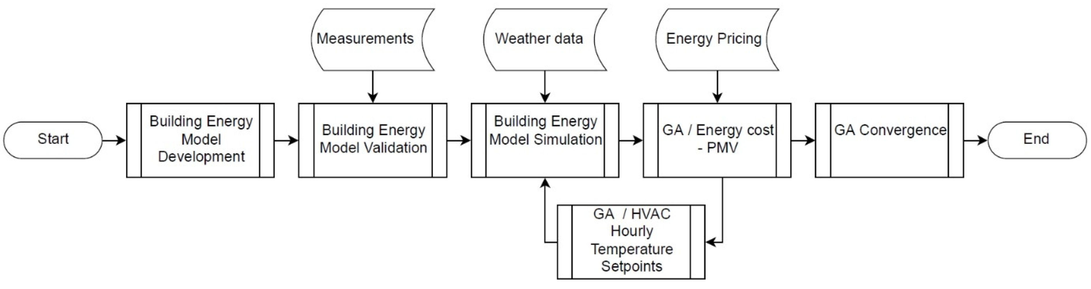
  • An original demand response optimization scheme is developed to include cost of energy and predicted mean vote (PMV) as the two criteria merged into one objective function. Along with HVAC hourly set points used as the variables of GA optimization, the developed approach constitutes a powerful assessment and decision tool which can be used to identify and ultimately apply dominant HVAC set point patterns based on actual weather conditions and preferences with regard to indoor conditions.
  • The optimization algorithm coupled with the validated dynamic thermal model of the building enables the assessment of energy cost, energy savings, and thermal comfort for a wide range of temperature set point patterns and RTP schemes.
  • The developed approach is designed to assess RTP schemes based on real DA market information to take advantage of price fluctuations which reflect current market operations in the optimization process.
In Section 2, the methodology and infrastructure of the case study building are presented. Results obtained during the optimization process are analyzed in Section 3. Finally, Section 4 highlights the main conclusions and recommendations for future work.

2. Methodology and Infrastructure

2.1. Methodology

The framework presented hereafter concerns optimization of the HVAC temperature set point schedule based on a genetic algorithm incorporating daily operational cost and the mean predicted mean vote (PMV) as the two criteria of the objective function. Operational cost refers to the cost of energy on the basis of the given day-ahead pricing profile and the HVAC energy consumption using the building’s validated model. The building thermal model is validated based on annual HVAC energy consumption and measurements of indoor temperature [34]. The validated thermal model of the building provides a reliable basis for this kind of investigation, as it takes into consideration the physical aspects of the building (geometry, materials), operational aspects, and climate conditions in a dynamic way. The baseline scenario is a reliable benchmark against which the optimized scenario is compared, since operational effects are kept constant to account for the fact that some operational effects such as user behavior, natural ventilation, and industrial operations are difficult to model and are in most cases not monitored. On the other hand, inducing changes in the temperature set points of the HVAC system makes it imperative to evaluate any solution on the basis of the building users’ thermal sensation and the heat exchange of the human body with the surrounding indoor environment. This balance of energy fluxes is influenced by physical activity, clothing, and the following indoor conditions; air temperature, mean radiant temperature, air velocity, and relative humidity (RH). Internal comfort is evaluated in this work using the PMV index as developed by Fanger in 1972 and adopted by ISO 7730 to account for human heat generation and exchange with the surrounding environment [35]. PMV is linked to the percentage of people dissatisfied (PPD) index to define the indoor conditions identified by most people (i.e. 90% or more) as thermally comfortable. Decision variables in the optimization process are the hourly HVAC temperature set points. Controlling HVAC temperature set points has, as a consequence, variations in the operation, power consumption, and running cost of the HVAC system. Naturally, this will impact indoor thermal conditions, which imposes the need for including thermal comfort as a criterion into the optimization process and compliance with established standards.
The methodology followed is depicted in Figure 1. Firstly, the building (Leaf Lab) three-dimensional (3D) thermal model was developed in Open Studio based on the technical information of the building (i.e., drawings, datasheets of systems installed) and site audits. Secondly, the model was validated using weather and indoor measurements (air temperature, RH) and HVAC power consumption. Details on the building modeling and validation procedures are available in Reference [34]. Thirdly, a new weather file was constructed by merging together weather measurements including dry and wet bulb temperature (°C), atmospheric pressure (kPa), relative humidity (%), dew point temperature (°C), global, normal and diffuse solar irradiance (Wh/2), and wind speed (m/s). The validated 3D thermal model of the building was used to simulate the building’s energy performance and obtain HVAC power demand (PHVAC, kW), indoor air temperature (Tair, °C), indoor radiant temperature (Trad, °C), and relative humidity (RH, %) for the period of interest (in this case, 2018). Fourthly, day-ahead pricing information was used to create the DARTP model required for the optimization. Day-ahead energy prices (€/MWh) for the region of central–northern Italy were used as the main component for the formulation of the energy pricing scheme used in the optimization. Additional costs related to transmission/distribution, as well as other costs and taxes, were included to define the final energy pricing profile. Fifthly, a genetic algorithm was constructed to optimize the objective function composed by (a) the daily sum of hourly cost of energy, and (b) the daily average of hourly PMV values for the working hours of the building and specifically from 9:00 a.m. to 6:00 p.m. In the GA optimization scheme, HVAC temperature set points were used as the discrete decision variables subject to upper and lower boundaries which differed between the heating and cooling seasons. Lastly, simulation of the validated building thermal model was executed in an iterative process using the set points selected by the GA until convergence criteria were met. Simulation output values of HVAC power, indoor air temperature, radiative temperature, and relative humidity were used to evaluate energy cost and the PMV at each iteration.

2.2. Infrastructure

Leaf Lab is one of the buildings of the Leaf Community smart microgrid in Angeli di Rosora in the province of Marche. Leaf Community is an industrial settlement owned and managed by Loccioni Group for conducting research and innovation in the energy, environment, automotive, aerospace, robotics, and other sectors. The Leaf Community is a unique blend of inspired qualified personnel where the preservation of the natural environment, RES, and worldwide R&D meets education, local culture, and society. Leaf Lab is a near-zero-energy industrial building of thermally insulated envelope walls with a U-value of 0.226 W/m2K and double-glazed windows with U-values between 1.793 and 3.194 W/m2K. It is equipped with an advanced energy management system controlling HVAC, artificial lights, energy from PV, and sensible thermal storage facilities. The building is equipped with a 236.5-kWp rooftop PV installation, a 400-m3 thermal storage water tank, ground water heat pumps (heating coefficient of performance (COP) of 4.8, cooling energy efficiency ratio (EER) of 6.2–7), smart artificial light controls based on illuminance/presence sensors, and automatic rotating external window louvers. Operations are monitored and managed by MyLeaf, a state-of-the-art proprietary energy management platform customized for testing and integrating new concepts and technologies.
According to the utility bills of the Leaf Community in 2018, the average unit cost of energy varied monthly between 0.1507 €/kWh and 0.1749 €/kWh, as shown in Figure 2. Furthermore, it is evident from the graph that the energy consumed outside the peak hours is significant and equal to 35.8%. The two-zone (peak/off-peak) ToU pricing scheme, however, offers low incentives for managing loads during daytime mainly as a consequence of monthly peak power charges.

2.2.1. GA optimisation model

The generic objective function of the GA optimization process is given by the equations below.
[ m i n ] f ( T s i = 1 24 ) = w c × i = 1 24 C i × P i i = 1 24 C i × P i b a s e l i n e + w p m v × i = 1 24 | P M V i | 24 × 3 ,
subject to | P M V i | 1 .
P i is obtained as an output by the simulation of the building’s thermal model and varies according to the building load and temperature set points.
PMV varies from −3 (cold) to +3 (hot) with zero being the optimum neutral value according to which internal heat production is equal to the loss of heat to the environment. PMV is calculated according to ISO 7730 based on the following parameters:
  • Metabolic (M) rate in W/m2;
  • Effective mechanical power (W) in W/m2;
  • Clothing insulation (Icl) in (m2K/W);
  • Air temperature in (°C);
  • Mean radiant temperature (°C);
  • Relative air velocity (m/s);
  • Relative humidity (RH, %).
For the purposes of the optimization, calculation of the PMV hourly values of air temperature, radiant temperature, and relative humidity were obtained as an output from the simulation of the building, while certain other parameters such as M , W , f c l , and p a , were considered to be constant. In the proposed algorithm, the normalized daily average of PMV hourly absolute values was used to search for optimal near-zero, positive, or negative values.
The genetic algorithm developed to optimize the objective function as expressed in Equation (1) was based on chromosomes of 24 discrete values (genes) each, corresponding to the temperature set points of the HVAC for hours 1–24 of the day. Chromosome values were subjected to upper and lower constraints depending on the season of the year. In heating season, genes T s i h = 8 18 during the working hours of the building (9:00 a.m. to 6:00 p.m.) had a lower boundary of 18 °C and an upper boundary of 24 °C. In cooling season, genes T s i c = 8 18 during working hours of the building had a low boundary of 20 °C and an upper boundary of 26 °C. This is mathematically expressed in the following constraints:
18 T s i h = 9 18 24 ; 20 T s i c = 9 18 26 .

2.2.2. Cost of energy model

The cost of energy model of the Leaf Community was developed in Matlab as described below. Based on current charges related to energy consumption as identified through energy bills for 2018, basic components were adjusted to incorporate day-ahead hourly price fluctuations in a DARTP scheme and to formulate the case study for advanced HVAC energy management. Overall, the developed hourly pricing scheme contained costs related to the consumption of energy, maximum power, grid services, taxes, and levies. Due to the fact that, in the current pricing scheme, a high share of the costs are determined by fixed charges, these costs were allocated a dynamic parameter to account for network flexibility and stability. The mathematical model of the energy cost is presented in the equations below.
C T = C E , T × ( 1 + I V A ) ;
C E , T = C S + C N + C E D D ;
C S = h = 0 24 E h v a c , h × ( D A h + C S , F ) ;
C N = C F + C P m a x + C A T + C A U C ;
C F + C A T + C A U C = h = 0 24 E h v a c , h × D A N , h × C F A A ;
C P m a x = max ( P h v a c , h ) × C P m a x , F ;
C E D D = h = 0 24 E h v a c , h × D A N , h × C E D H .

3. Results and Discussion

The generic GA optimization scheme analyzed in the previous section was applied to include working hours (9:00 a.m. to 6:00 p.m.) plus two hours before (7:00–9:00 a.m.) and two hours after (6:00–8:00 p.m.). This was considered essential to study the effects of preheating or precooling of the building and maintaining internal conditions at sensible temperature values for some time after working hours to account for the fact that some people may still occupy the building. Optimization was conducted for the main industrial thermal zone of the building, which occupies a total area of 1327 m2 and a height of 8 m, surrounded by various other spaces including offices, meeting rooms, and other facilities on two floors. Following a number of trials, the population size of the GA was set to 50, the crossover fraction was set to 0.8, and the maximum number of iterations was set to 4,600 in order to examine a wide range of different solutions. Based on the set of the results, solutions were obtained to identify the set point patterns associated with optimum levels of energy and cost savings, as well as compliance with well-established standards of thermal comfort and temperature set point drift. The approach was designed to evaluate energy cost on a 24-h time frame. Representative results for four winter days, two days for autumn, one for summer, and one for spring are presented to account for different seasonal climatic conditions, heating and cooling modes, and DA pricing profiles.
Scenario 1: 25 January 2018 (Winter)
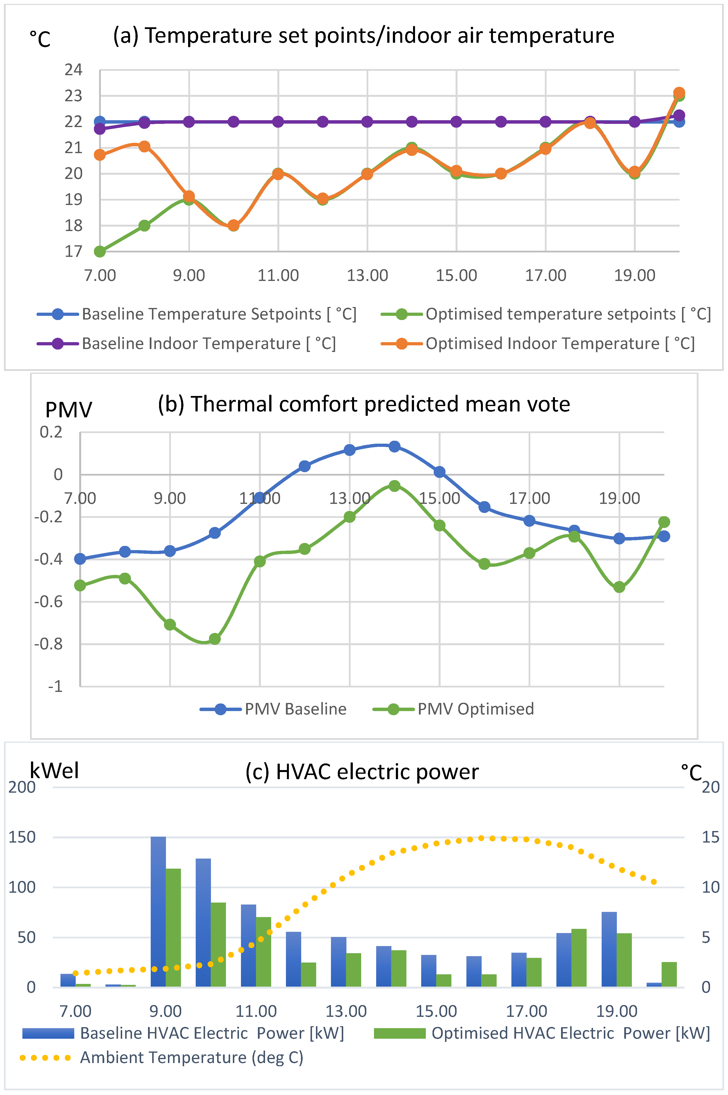
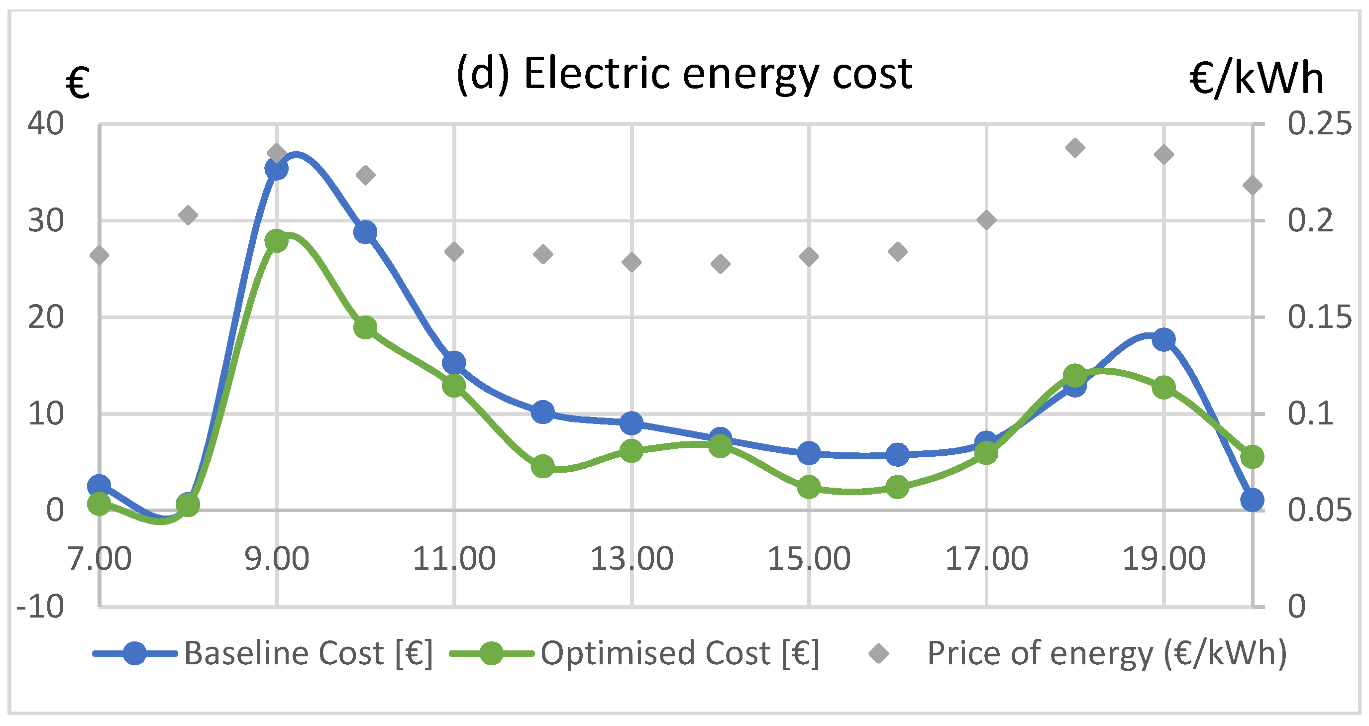
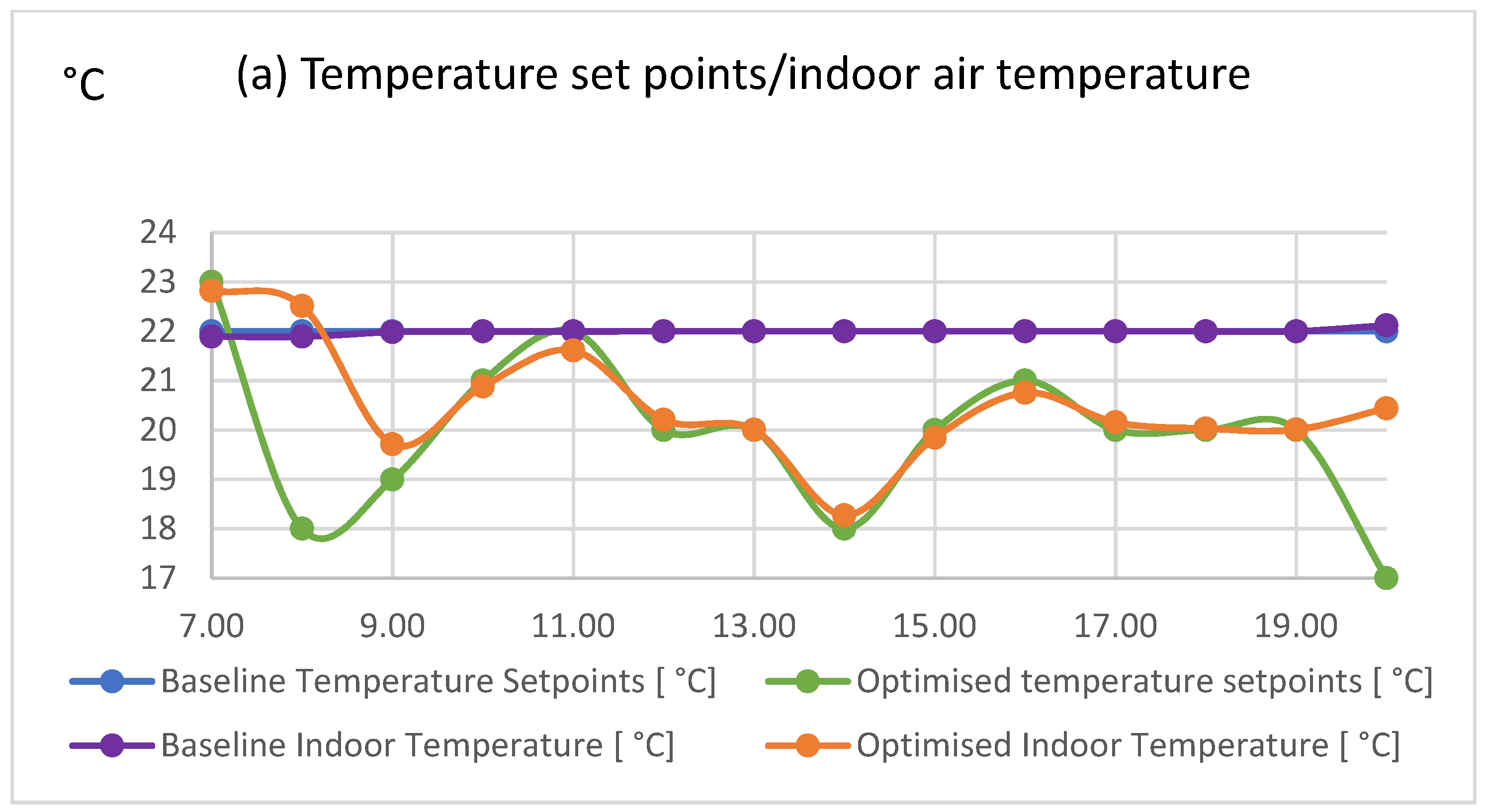
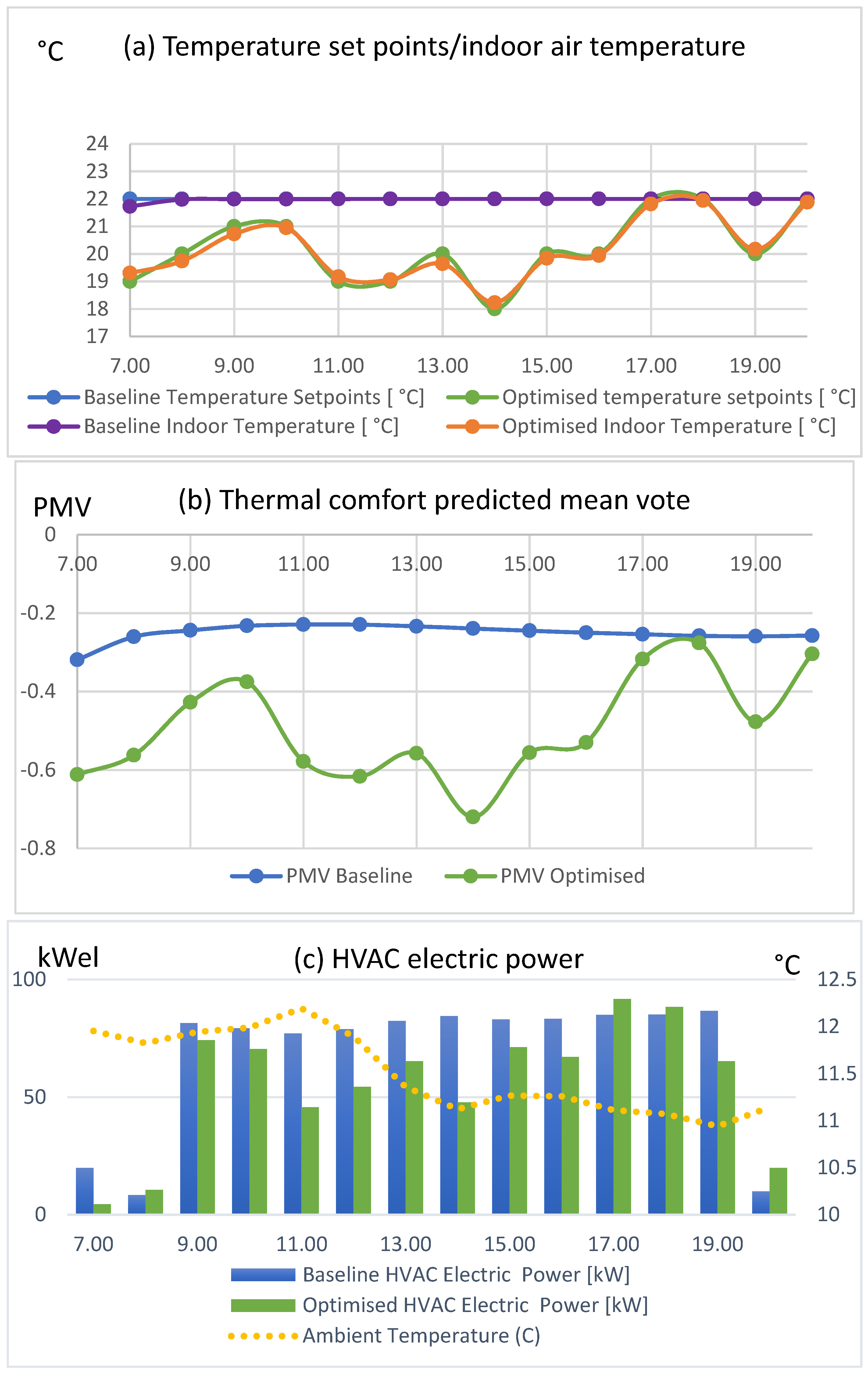
Results from the GA HVAC optimization on 25 January 2018 are presented in Figure 3 below. In the optimized scenario of this case, set points during working hours were selected, on an hourly basis, to be between 18 °C and 22 °C, as shown in Figure 3a, and the energy of the HVAC was reduced from 759.88 kWh to 570.13 kWh, a reduction of 25% (Figure 3c). Energy cost (Figure 3d) was decreased from €159.3 to €121.03, which is equal to 25.0% savings. The HVAC power was kept lower in the optimized scenario, except during hours 6:00 and 8:00 p.m. At the baseline scenario, the PMV varied from −0.36 to 0.13, while, at the optimized scenario, from −0.78 to −0.05 (Figure 3b). The average PMV varied from −0.14 to −0.38, which corresponds to a PPD increase from 6.28% to 9.13% between the baseline and optimized scenario. In this case, a trade-off between thermal comfort and energy consumption was found to be associated with significant cost savings at times of high pricing rates but also during low pricing zones.
Scenario 2: 27 March 2018 (Spring)
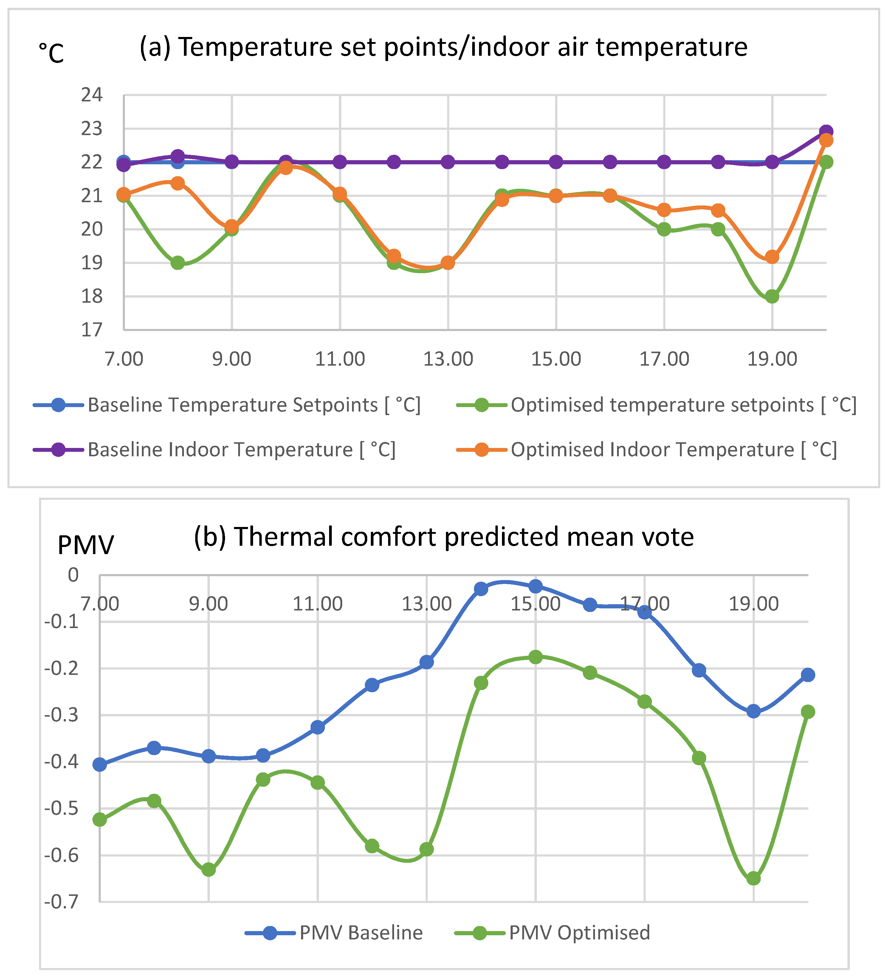
Results from the GA HVAC optimization on 27 March 2018 are presented in Figure 4 below. In the optimized scenario of this case, set points were dynamically altered between 19 °C and 22 °C within working hours (Figure 4a), and the energy of the HVAC was reduced from 610.91 kWh to 463.43 kWh (Figure 4c), a reduction of 24.1%. Energy cost (Figure 4d) was decreased from €121.02 to €94.05, which is equal to 22.3% savings. The HVAC power was lower in the optimized scenario, except during hours 10:00 a.m. and 8:00 p.m. (outside working hours). At the baseline scenario, the PMV varied from −0.39 to −0.02, while, at the optimized scenario, PMV varied from −0.65 to −0.18 (Figure 4b). The average PMV varied from −0.2 to −0.41, which corresponds to a PPD increase from 6.47% to 9.28% between the baseline and optimized scenario. Similarly, in this case, cost savings occurred mostly early in the morning and late in the evening when prices were relatively high. Some savings were also observed around 12:00–1:00 p.m. just before prices got to the lowest level of that particular day.
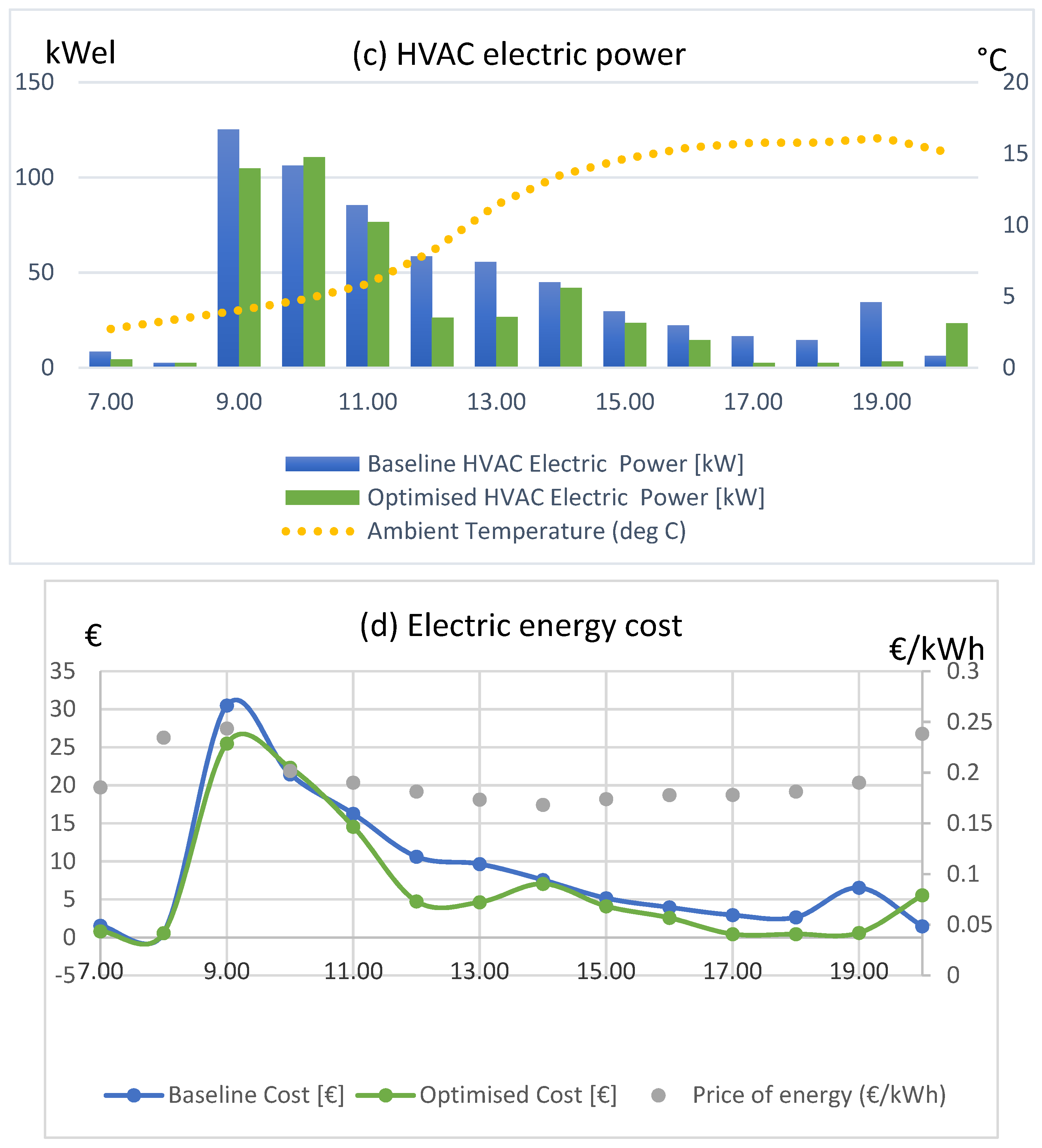
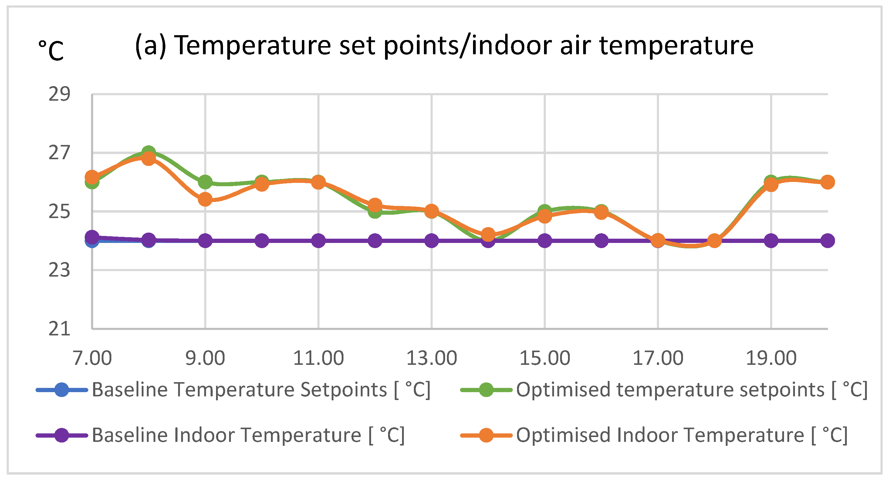
Scenario 3: 15 August 2018 (Summer)
Results from the GA HVAC optimization on 15 August 2018 are presented in Figure 5 below. In the optimized scenario, temperature set points varied, on an hourly basis, from 26 °C to 24 °C, within working hours (Figure 5a), whereas the energy of the HVAC (Figure 5c) was reduced from 1447.83 kWh to 1175.93 kWh, a reduction of 18.8%. Energy cost (Figure 5d) was decreased from €295.26 to €238.57, which is equal to 19.2% savings. The mean PMV for working hours was improved from −0.2 to −0.007, and the PPD was decreased from 6.42% to 5.03%. In the optimized solution, HVAC power was lower during all hours except 2:00, 5:00, and 6:00 p.m. following the set points changing from higher to lower values down to 24 °C. In this scenario, cost savings occurred throughout the day, while they were more evident during hours of high prices compared to neighbor regions. The PMV was improved as the fixed cooling set point caused thermal discomfort and unnecessary high energy consumption levels for most hours during the day.
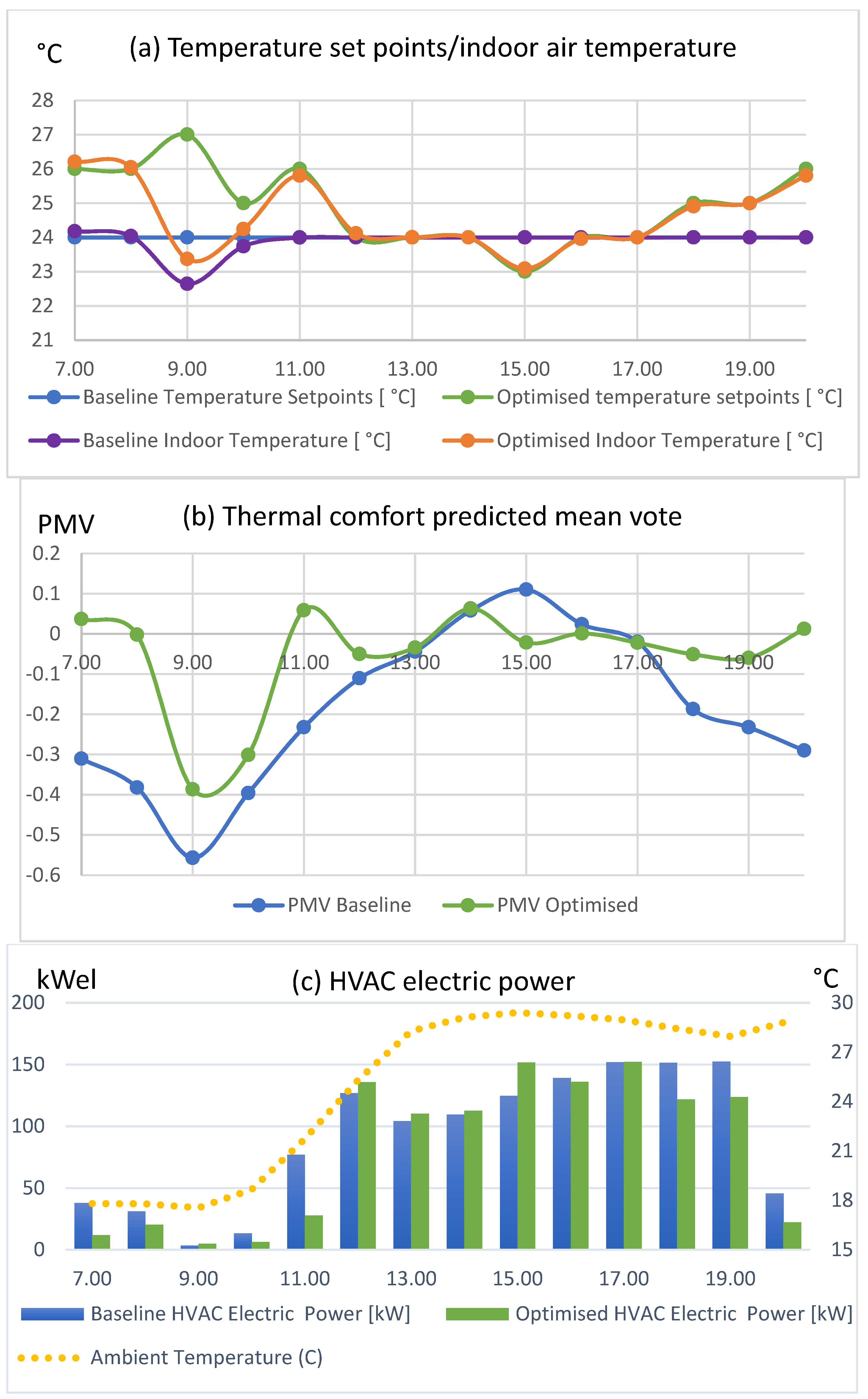
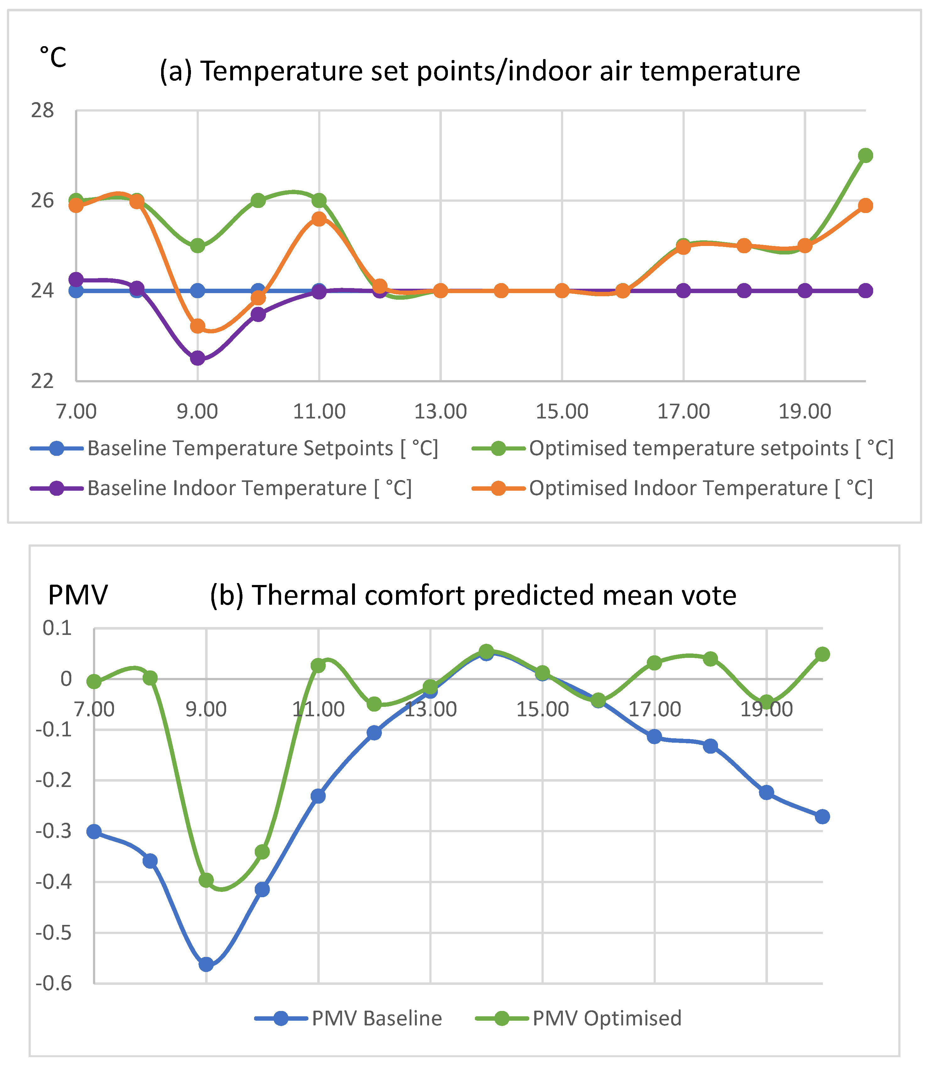
Scenario 4: 10 September 2018 (Autumn)
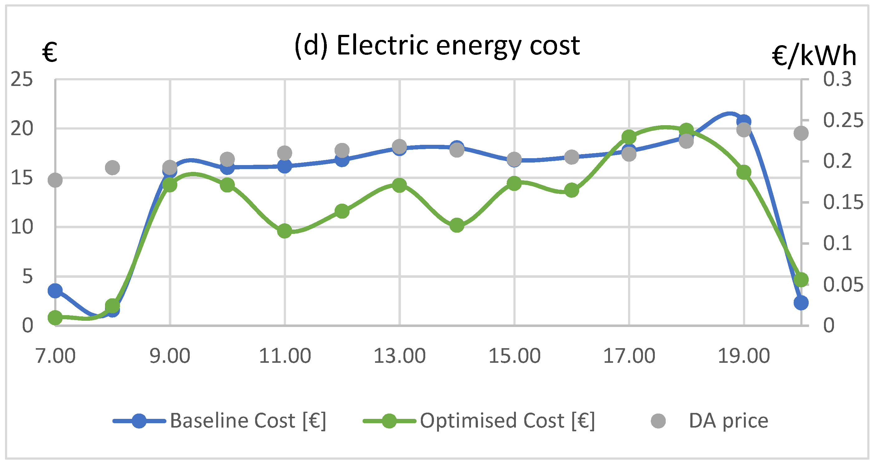
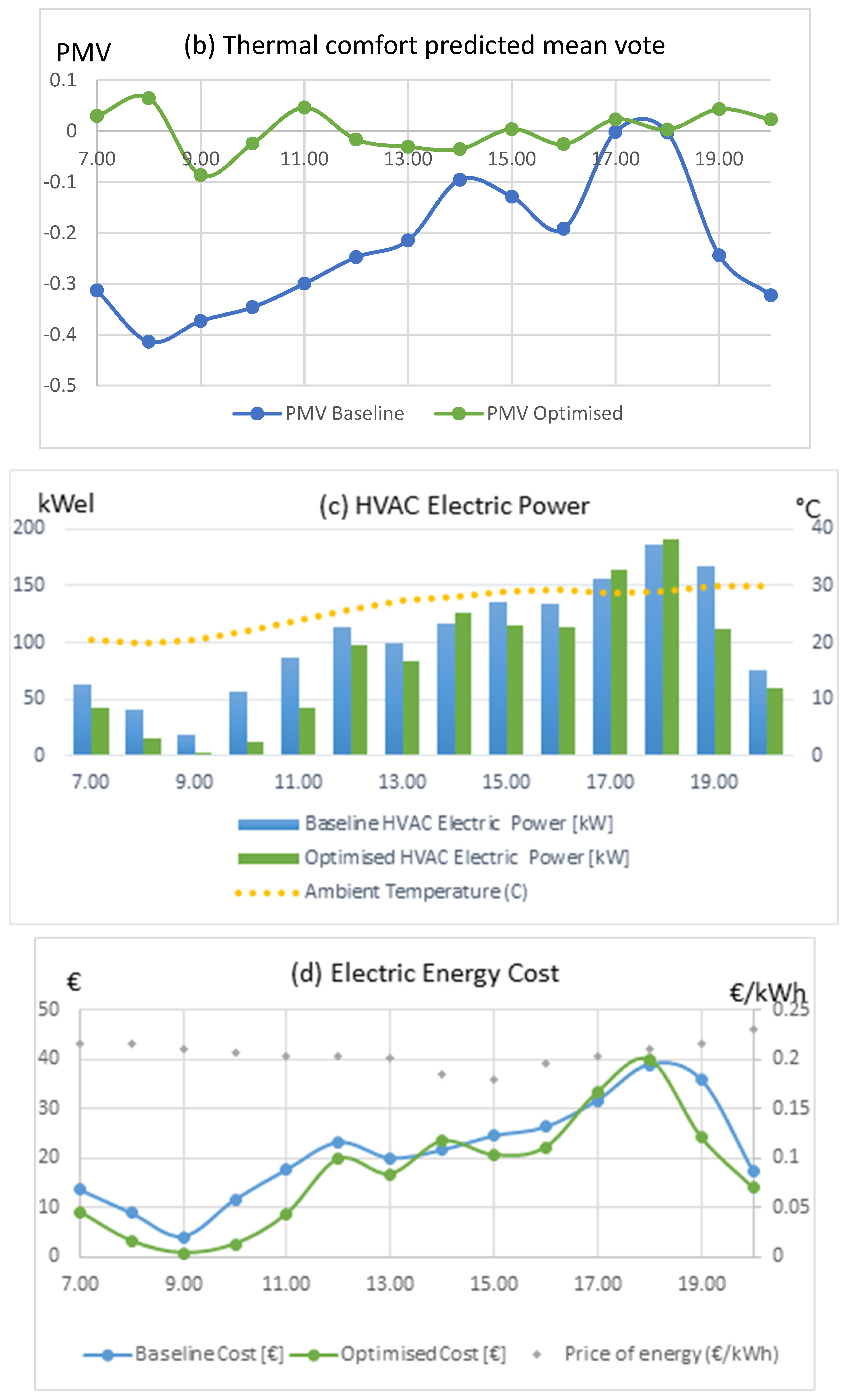
Scenario 4 results from the GA HVAC optimization on 10 September 2018 are presented in Figure 6 below. In this case, the energy of the HVAC (Figure 6c) was reduced from 1268.47 kWh to 1136.29 kWh, a reduction of 10.4%, while energy cost (Figure 6d) was decreased from €311.59 to €280.68, a reduction of 9.9%. The slight difference in the mean PMV for working hours from −0.144 to −0.073 corresponds to a PPD decrease by 1.1%. The PMV at the baseline scenario varied from −0.56 up to 0.11, while, in the optimized scenario, PMV varied from −0.39 to 0.06 (Figure 6b). HVAC power values (Figure 6c) in the optimized scenario exceeded their respective values in the baseline scenario at times of low prices with respect to the neighboring regions and specifically from 12:00–3:00 p.m. Baseline energy consumption was unnecessarily high during morning hours as it coincided with significant negative PMV levels, while efficient performance was observed in the optimized scenario where the set point was kept at the highest allowed level. Indoor temperature (Figure 6a) deviated from the set point temperature for both the baseline and the optimized scenario between 9:00 and 10:00 a.m. In the optimized scenario, the HVAC energy consumption remained at low levels due to the negative PMV levels during the same time period. Another interesting observation was that the PMV in the baseline scenario significantly increased over time during the day, despite the fact that the indoor temperature was kept constant, which was mainly due to the effect of radiative temperature on thermal comfort.
Scenario 5: 21 September 2018 (Autumn)
Results from the GA HVAC optimization on 21 September 2018 are presented in Figure 7 below. In the optimized scenario, set points within working hours fluctuated between 26 °C and 24 °C (Figure 7a), while the energy of the HVAC was reduced from 1248.69 kWh to 1078.16 kWh (Figure 7c), a reduction of 13.7%. Energy cost (Figure 7d) was decreased from €298.07 to €253.79, which is equal to savings of 14.9%. The mean PMV for working hours was improved from −0.172 to −0.056, and the respective PPD was decreased from 6.4% to 5.4%. In this case, the optimized PMV (Figure 7b) reflected improved thermal conditions, since it oscillated in the region −0.40 to 0.05 in the optimized scenario, while, in the baseline scenario, it varied between −0.56 and 0.05. Energy savings were achieved by keeping the temperature set points at higher levels, while the PMV was at negative levels during early morning and late afternoon working hours. Slightly higher HVAC power levels (Figure 7c) were observed during hours 12:00–3:00 p.m., coinciding with the lowest energy prices during the day.
Scenario 6: 20 November 2018 (Winter)
Results from the GA HVAC optimization on 20 November 2018 are presented in Figure 8 below. Temperature set points in the optimized scenario were dynamically controlled from 17 °C to 23 °C (18 °C to 22 °C within working hours; Figure 8a). In the optimized scenario, the energy of the HVAC was reduced from 923.75 kWh to 756.67 kWh, a reduction of 18.1% (Figure 8c). Energy cost, shown in Figure 8d, was decreased from €217.33 to €177.66, which is equal to savings of 17.4%. PMV in the optimized scenario varied from −0.50 to −0.10, whereas, in the baseline scenario, it varied between −0.07 and −0.05 (Figure 8b). The mean PMV for working hours was increased from −0.055 to −0.276, and the respective PPD was increased by 1.4%. PMV was kept at small negative values and above −0.3 for most hours, except for 2:00 and 3:00 p.m., where PMV was −0.49 and −0.35, respectively. HVAC power in the optimized scenario was kept at lower levels compared to the baseline for all working hours (except early morning hours).
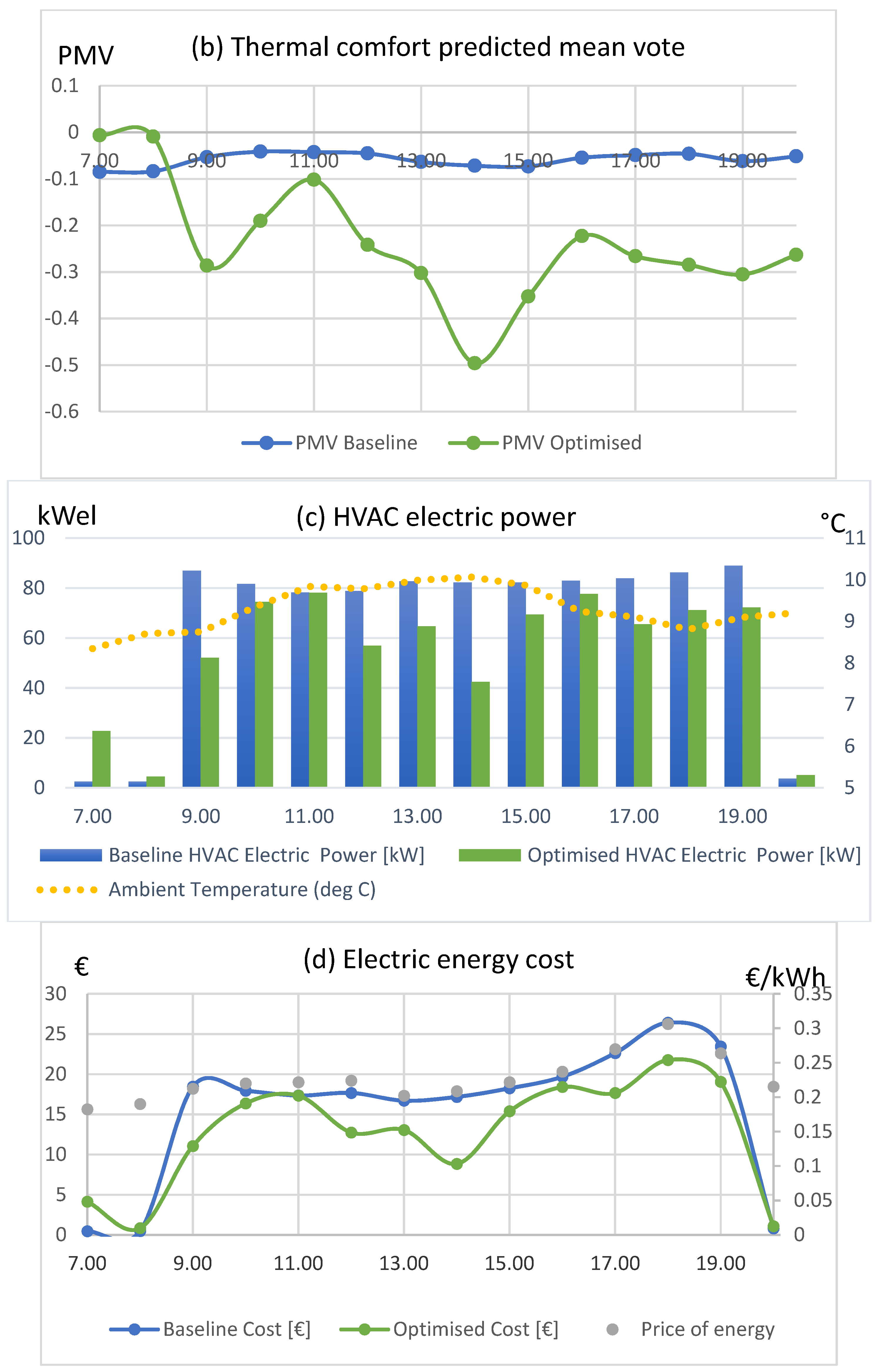
Scenario 7: 22 November 2018 (Winter)
Results from the GA HVAC optimization on 22 November 2018 are presented in Figure 9 below. Optimized temperature set points, as presented in Figure 9a, varied from 19 °C to 22 °C. In the optimized scenario, the energy of the HVAC was reduced from 717.77 kWh to 631.61 kWh, a reduction of 12.0% (Figure 9c). Energy cost (Figure 9d) was decreased from €179.59 to €159.01, which is equal to savings of 11.5%. PMV in the optimized scenario (
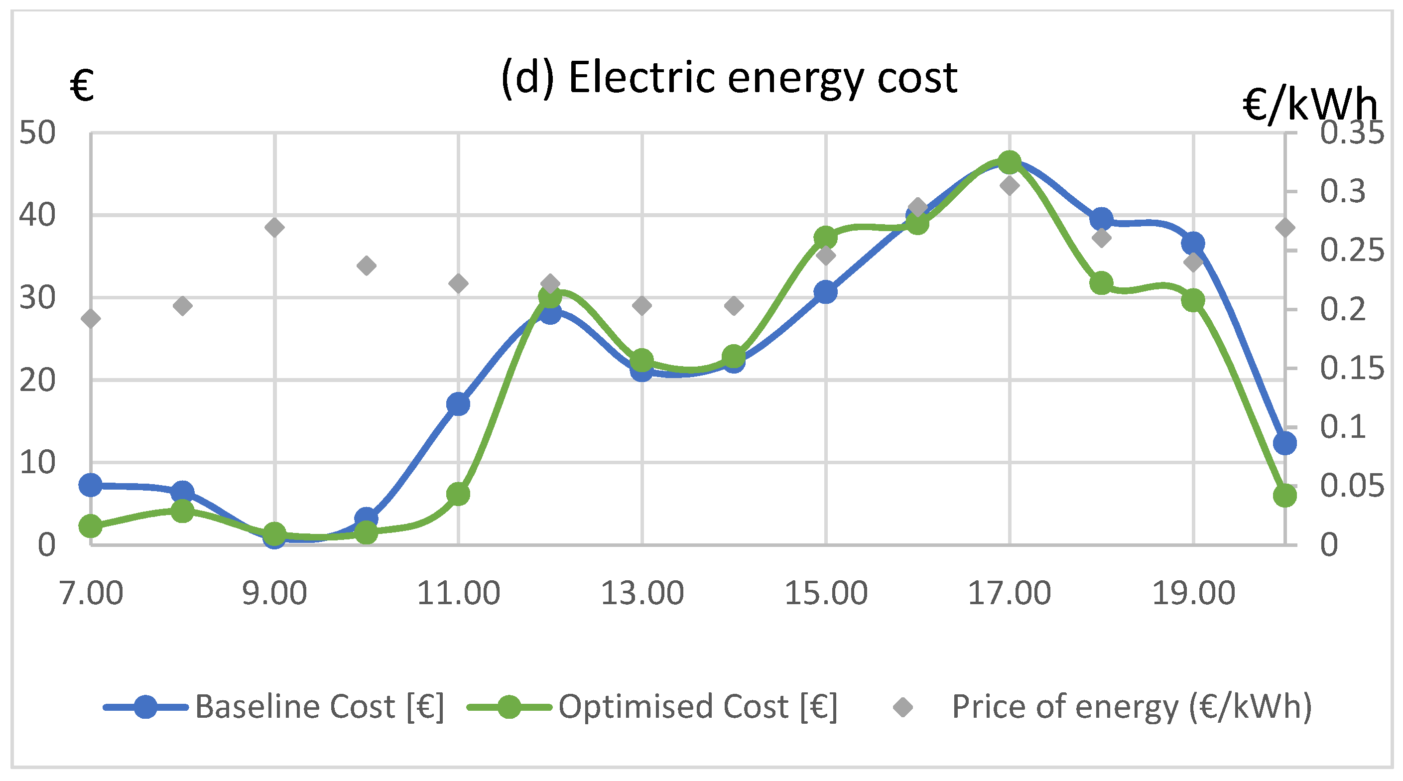
Figure 9b) varied between −0.25 and −0.01 and, in the baseline scenario, PMV varied between −0.03 and −0.01. The mean PMV for working hours was increased from −0.016 to −0.110, and the respective PPD was increased by 0.4%. Significant energy savings occurred during hours of high prices, corresponding to hours 9:00 a.m., 1:00 p.m., and 3:00–6:00 p.m., while the PMV was kept at small negative levels down to −0.25.
Scenario 8: 25 November 2018 (Winter)
Optimization results for HVAC optimization on 25 November 2018 are available in Figure 10. Temperature set points varied from 18 °C to 22 °C in the optimized solution (Figure 10a). In this scenario, HVAC energy consumption (Figure 10c) was reduced from 944.85 kWh to 776.17 kWh, a decrease of 17.9% compared to the baseline. Daily cost (Figure 10d) was reduced from €199.52 to €164.26, a reduction of 17.7%. The mean PMV was decreased from −0.244 in the baseline scenario to −0.478, which is equivalent to a PPD increase of 4.2% (Figure 10b). HVAC consumption in the optimized scenario exceeded the baseline levels slightly during hours 8:00 a.m., and 5:00 and 6:00 p.m. A compromise between maintaining comfort within tolerable levels while maximizing cost savings was reached.

4. Conclusions and Future Steps

The developed approach provides an optimization assessment framework for HVAC energy management in day-ahead real-time pricing demand response programs. In this framework, a GA-based approach was developed to investigate DR implementation for a near-zero-energy industrial building located in the region of Marche in Italy. Results indicate that there is significant potential for energy and cost savings by controlling indoor conditions within acceptable levels of thermal comfort as evaluated according to predicted mean vote. Several scenarios were analyzed to demonstrate a realistic potential of cost of energy reductions in the range between 9.9% and 25%, whereas the reduction of HVAC energy consumption varied between 10.4% and 25%. Presented solutions within established standard requirements for indoor comfort and indoor temperature drift rate were selected for evaluation from a wide range of available solutions. The proposed demand response approach is applicable in a wide range of building energy optimization assessment schemes due to the fact that it deploys temperature set point levels for HVAC control. It can be applied to establish optimal control of thermal zones in buildings of various uses and sizes controlled by single or distributed thermostatic controls. It was demonstrated that there is an unexplored potential for HVAC dynamic control associated with demand response RTP schemes which could be intelligently embedded in the operation of such systems and smart grids in the years to come. The computational cost of the proposed approach was significant, as, at this stage of the research, a high number of iterations (4600) were performed to ensure the search was as extensive and deep as possible. However, based on the results obtained, there is great potential for reducing the time for GA convergence, since satisfactory near-optimal results were, in most cases, obtained in the first day of the run (total average time for a conventional personal computer (PC) was approximately two days). Furthermore, a careful adjustment of optimization parameters and constraints combined with weather predictions, along with the evolution of computer resources and microprocessor capabilities, can make the proposed approach deployable in real time in the near future. In addition, future research could involve the investigation of a typology of HVAC near-optimal set point configurations in response to patterns in ambient conditions. Experimental research could entail the testing of optimal set point patterns in real conditions as a next step toward the actual implementation of the developed methodology.

Author Contributions

Conceptualization, N.K. and D.K.; Data curation, N.S., K.G. and D.I.; Formal analysis, N.K.; Funding acquisition, N.K., D.K. and C.C.; Investigation, N.K., N.S. and D.K.; Methodology, N.K., N.S. and D.K.; Project administration, N.K., D.K., D.I. and C.C.; Resources, D.K., K.G., K.K., D.I. and C.C.; Software, N.K., N.S. and K.G.; Supervision, D.K., K.K. and C.C.; Validation, N.S. and D.K.; Visualization, N.K. and N.S.; Writing – original draft, N.K.; Writing – review & editing, N.K., N.S., D.K., K.K., D.I. and C.C.

Funding

This research received funding from the European Union’s Horizon 2020 research and innovation program under the Marie Skłodowska-Curie grant agreement No. 645677.

Conflicts of Interest

The authors declare no conflict of interest.

Nomenclature

T s i = 1 24 hourly temperature set points of the HVAC system the next day
w c weighting coefficient for the daily operational cost of energy for the HVAC
w p m v weighting coefficient for the daily thermal comfort
C i day-ahead price per hour for hours 1–24
P i hourly average power consumption of the HVAC in kW (equivalent to kWh)
C T total energy bill (€)
IVAvalue added tax (€)
C E total energy charges (€)
C T total tax charges (€)
C S energy procurement cost (€)
C N network services cost (€)
C S , F energy procurement fixed cost component (€/kWh)
C E D D daily excise duty on electricity and taxes (€)
C v , u various costs normalized per kWh (€/Wh)
D A h day-ahead market prices (€/kWh)
C F fixed cost component (€)
C P m a x maximum power cost component (€/kW)
C A T active energy cost component (€/kWh)
C A U C fixed cost for up to 4 GWh per month (€/kWh)
D A N , h DA price flexible factor per hour h (€/kWh)
C E D H excise duty per kWh (€/kWh)
C F A A parameter to account for F, AT, and A-UC components (€/kWh)
C P m a x , F maximum power fixed cost component (€/kW)
Abbreviations
ADRautomated demand response
AMIadvanced metering infrastructure
COPcoefficient of performance
CPPcritical peak pricing
DAday-ahead
DERdistributed energy resources
DRdemand response
DSMdemand side management
EERenergy efficiency ratio
GAgenetic algorithm
HVACheating, ventilation, and air conditioning
MIPMixed Integer Programming
MILPmixed-integer linear problem
MINLPmixed-integer non-linear problem
PMVpredicted mean vote
PPDpercentage of people dissatisfied
PVphotovoltaic
RESrenewable energy sources
RHrelative humidity
RTPreal-time pricing
R&DResearch and Development
SDGsustainable development goal
ToUtime of use

References

  1. Albadi, M.H.; El-Saadany, E.F. A summary of demand response in electricity markets. Electr. Power Syst. Res. 2008, 78, 1989–1996. [Google Scholar] [CrossRef]
  2. Siano, P. Demand response and smart grids—A survey. Renew. Sustain. Energy Rev. 2014, 30, 461–478. [Google Scholar] [CrossRef]
  3. Mccollum, D.; Gomez, L.; Riahi, E.K.; Parkinson, S. A Guide to SDG Interactions: From Science to Implementation. 2017. Available online: http://www.icsu.org/publications/a-guide-to-sdg-interactions-from-science-to-implementation (accessed on 1 April 2019).
  4. Palensky, P.; Dietrich, D. Demand side management: Demand response, intelligent energy systems, and smart loads. IEEE Trans. Ind. Inf. 2011, 7, 381–388. [Google Scholar] [CrossRef]
  5. Doostizadeh, M.; Ghasemi, H. A day-ahead electricity pricing model based on smart metering and demand-side management. Energy 2012, 46, 221–230. [Google Scholar] [CrossRef]
  6. Li, Y.; Yang, Z.; Zhao, D.; Lei, H.; Cui, B.; Li, S. Incorporating energy storage and user experience in isolated microgrid dispatch using a multi-objective model. IET Renew. Power Gener. 2019, 13, 973–981. [Google Scholar] [CrossRef]
  7. Li, Y.; Yang, Z.; Li, G.; Mu, Y.; Zhao, D.; Chen, C.; Shen, B. Optimal scheduling of isolated microgrid with an electric vehicle battery swapping station in multi-stakeholder scenarios: A bi-level programming approach via real-time pricing. Appl. Energy 2018, 232, 54–68. [Google Scholar] [CrossRef] [Green Version]
  8. Good, N.; Ellis, K.A.; Mancarella, P. Review and classification of barriers and enablers of demand response in the smart grid. Renew. Sustain. Energy Rev. 2017, 72, 57–72. [Google Scholar] [CrossRef] [Green Version]
  9. Vallés, M.; Reneses, J.; Cossent, R.; Frías, P. Regulatory and market barriers to the realization of demand response in electricity distribution networks: A European perspective. Electr. Power Syst. Res. 2016, 140, 689–698. [Google Scholar] [CrossRef]
  10. Torriti, J.; Hassan, M.G.; Leach, M. Demand response experience in Europe: Policies, programmes and implementation. Energy 2010, 35, 1575–1583. [Google Scholar] [CrossRef] [Green Version]
  11. OpenADR 2.0 Demand Response Program Implementation Guide. OpenADR Alliance 2014, 1–91.
  12. Faruqui, A.; Hledik, R.; George, S.S.; Bode, J.; Mangasarian, P.; Rohmund, I.; Wikler, G.; Ghosh, D.; Yoshida, S. A National Assessment of Demand Response Potential; FERC: Washington, DC, USA, 2009.
  13. Shariatzadeh, F.; Mandal, P.; Srivastava, A.K. Demand response for sustainable energy systems: A review, application and implementation strategy. Renew. Sustain. Energy Rev. 2015, 45, 343–350. [Google Scholar] [CrossRef]
  14. Vardakas, J.; Zorba, N.; Verikoukis, C. A Survey on Demand Response in Smart Grids. IEEE Trans. Ind. Inf. 2015, 11, 1–8. [Google Scholar]
  15. Motegi, N.; Piete, M.A.; Watson, D.S.; Kiliccote, S.; Xu, P. Introduction to Commercial Building Control Strategies and Techniques for Demand Response; Lawrence Berkeley National Laboratory: Berkeley, CA, USA, 2007.
  16. Mathieu, J.L. Modeling, Analysis, and Control of Demand Response Resources. Ph.D Thesis, University California, Berkeley, CA, USA, 2012. [Google Scholar] [Green Version]
  17. Goldman, C.; Reid, M.; Levy, R.; Silverstein, A. National Action Plan for Energy Efficiency, Coordination of Energy Efficiency and Demand Response. 2010. Available online: https://www.epa.gov/sites/production/files/2015-08/documents/ee_and_dr.pdf (accessed on 7 June 2019).
  18. Pérez-Lombard, L.; Ortiz, J.; Pout, C. A review on buildings energy consumption information. Energy Build. 2008, 40, 394–398. [Google Scholar] [CrossRef]
  19. Dounis, A.I.; Caraiscos, C. Advanced control systems engineering for energy and comfort management in a building environment—A review. Renew. Sustain. Energy Rev. 2009, 13, 1246–1261. [Google Scholar] [CrossRef]
  20. Harish, V.S.K.V.; Kumar, A. A review on modeling and simulation of building energy systems. Renew. Sustain. Energy Rev. 2016, 56, 1272–1292. [Google Scholar] [CrossRef]
  21. Afram, A.; Janabi-Sharifi, F. Review of modeling methods for HVAC systems. Appl. Therm. Eng. 2014, 67, 507–519. [Google Scholar] [CrossRef]
  22. Afroz, Z.; Shafiullah, G.M.; Urmee, T.; Higgins, G. Modeling techniques used in building HVAC control systems: A review. Renew. Sustain. Energy Rev. 2018, 83, 64–84. [Google Scholar] [CrossRef]
  23. Okochi, G.S.; Yao, Y. A review of recent developments and technological advancements of variable-air-volume (VAV) air-conditioning systems. Renew. Sustain. Energy Rev. 2016, 59, 784–817. [Google Scholar] [CrossRef]
  24. Wang, S.; Ma, Z.; Wang, S. Supervisory and Optimal Control of Building HVAC Systems: A Review Supervisory and Optimal Control of Building HVAC Systems: A Review. HVAC R Res. 2008, 14, 3–32. [Google Scholar] [CrossRef]
  25. Lin, H.-W.; Hong, T. On variations of space-heating energy use in office buildings. Appl. Energy 2013, 111, 515–528. [Google Scholar] [CrossRef] [Green Version]
  26. Papantoniou, S.; Kolokotsa, D.; Kalaitzakis, K. Building optimization and control algorithms implemented in existing BEMS using a web based energy management and control system. Energy Build. 2015, 98, 45–55. [Google Scholar] [CrossRef]
  27. Risbeck, M.J.; Maravelias, C.T.; Rawlings, J.B.; Turney, R.D. A mixed-integer linear programming model for real-time cost optimization of building heating, ventilation, and air conditioning equipment. Energy Build. 2017, 142, 220–235. [Google Scholar] [CrossRef]
  28. Pombeiro, H.; Machado, M.J.; Silva, C. Dynamic programming and genetic algorithms to control an HVAC system: Maximizing thermal comfort and minimizing cost with PV production and storage. Sustain. Cities Soc. 2017, 34, 228–238. [Google Scholar] [CrossRef]
  29. Serra, J.; Pubill, D.; Vázquez, M.Á.; Verikoukis, C. Experimental evaluation of an HVAC system under dynamic pricing with comfort constraints. In Proceedings of the 2014 IEEE PES Innov. Smart Grid Technol. Conf. ISGT 2014, Washington, DC, USA, 19–22 February 2014. [Google Scholar]
  30. Alhaider, M.; Fan, L. Mixed integer programming for HVACs operation. IEEE Power Energy Soc. Gen. Meet. 2015, 2015, 1–5. [Google Scholar]
  31. Ma, K.; Yuan, C.; Yang, J.; Liu, Z.; Guan, X. Switched Control Strategies of Aggregated Commercial HVAC Systems for Demand Response in Smart Grids. Energies 2017, 10, 953. [Google Scholar] [CrossRef]
  32. Lee, Y.M.; Horesh, R.; Liberti, L. Simulation and optimization of energy efficient operation of HVAC system as demand response with distributed energy resources. In Proceedings of the 2015 Winter Simulation Conference (WSC), Huntington Beach, CA, USA, 6–9 December 2015; pp. 991–999. [Google Scholar]
  33. Zhang, Y.; Zeng, P.; Zang, C. Multi-objective optimal control algorithm for HVAC based on particle swarm optimization. In Proceedings of the Fifth International Conference on Intelligent Control and Information Processing, Dalian, China, 18–20 August 2014; pp. 417–423. [Google Scholar]
  34. Kampelisa, N.; Gobakisa, K.; Vagiasa, V.; Kolokotsaa, D.; Standardib, L.; Isidorib, D.; Cristallib, C.; Montagninocd, F.M.; Paredescd, F.; Muratore, P. Evaluation of the performance gap in industrial, residential & tertiary near-Zero energy buildings. Energy Build. 2017, 148, 58–73. [Google Scholar] [Green Version]
  35. EN ISO 7730. Ergonomics of the Thermal Environment—Analytical Determination and Interpretation of Thermal Comfort using Calculation of the PMV and PPD Indices and Local Thermal Comfort Criteria (ISO 7730:2005). CEN, 2006. Available online: https://www.iso.org/standard/39155.html (accessed on 7 June 2019).
Figure 1. Genetic algorithm (GA)-based heating, ventilation, and air conditioning (HVAC) temperature set point optimization scheme.
Energies 12 02177 g001
Figure 2. Leaf Community electrical energy consumption and unit cost of energy in 2018.
Energies 12 02177 g002
Figure 3. GA HVAC optimization results for 25 January 2018 (winter).
Energies 12 02177 g003aEnergies 12 02177 g003b
Figure 4. GA HVAC optimization results for 27 March 2018 (spring).
Energies 12 02177 g004aEnergies 12 02177 g004b
Figure 5. GA HVAC optimization results for 15 August 2018 (summer).
Energies 12 02177 g005aEnergies 12 02177 g005b
Figure 6. GA HVAC optimization results for 10 September 2018 (autumn).
Energies 12 02177 g006aEnergies 12 02177 g006b
Figure 7. GA HVAC optimization results for 21 September 2018 (autumn).
Energies 12 02177 g007aEnergies 12 02177 g007b
Figure 8. GA HVAC optimization results for 20 November 2018 (winter).
Energies 12 02177 g008aEnergies 12 02177 g008b
Figure 9. GA HVAC optimization results for 22 November 2018 (winter).
Energies 12 02177 g009
Figure 10. GA HVAC optimization results for 25 November 2018 (winter).
Energies 12 02177 g010aEnergies 12 02177 g010b

