Abstract
This paper proposes an improved feedback algorithm by binary particle swarm optimization (BPSO)-based nonsingular terminal sliding mode control (NTSMC) for DC–AC converters. The NTSMC can create limited system state convergence time and allow singularity avoidance. The BPSO is capable of finding the global best solution in real-world application, thus optimizing NTSMC parameters during digital implementation. The association of NTSMC and BPSO extends the design of classical terminal sliding mode to converge to non-singular points more quickly and introduce optimal methodology to avoid falling into local extremum and low convergence precision. Simulation results show that the improved technique can achieve low total harmonic distortion (THD) and fast transients with both plant parameter variations and sudden step load changes. Experimental results of a DC–AC converter prototype controlled by an algorithm based on digital signal processing have been shown to confirm mathematical analysis and enhanced performance under transient and steady-state load conditions. Since the improved DC–AC converter system has significant advantages in tracking accuracy and solution quality over classical terminal sliding mode DC–AC converter systems, this paper will be applicable to designers of relevant robust control and optimal control technique.
1. Introduction
DC–AC converters have been widely applied in renewable energy systems, such as solar photovoltaic (PV) energy systems, wind turbine generator systems and fuel cell power generation systems. For example, a solar PV energy system can convert sunlight into usable electrical energy. The simplified solar PV systems include PV panels, DC–DC converters, DC–AC converters and loads. Such system can be designed to yield maximum power delivered to the load. There are two power conversion stages in this structure, so it can be considered a two-stage system. The DC–DC converter is used to handle maximum power point tracking (MPPT) and regulate the DC load voltage. At the same time as the grid connection occurs, the power is generated by the PV panel and converted to AC power by the DC–AC converter. Furthermore, the operation of DC–AC conversion and maximum power point tracking (MPPT) can be combined into a single-stage system using only one DC–AC converter. In various power converter topologies for renewable energy applications, inductor capacitor (LC) filter DC–AC converters are often used as an interface between renewable energy and the grid. The converter DC link is connected to the PV panel either directly or through an intermediate DC–DC power conversion stage. The LC low-pass filter eliminates higher harmonics in the converter’s pulse width modulation (PWM) output, enabling pure sine. Therefore, even under plant parametric variations and external load disturbances, the requirements of high-performance DC–AC converters must involve fast dynamic response and low total harmonic distortion (THD) of the output voltage. In order to meet these requirements, a proportional plus integral (PI) controller is frequently used; nevertheless, the controller may not be able to withstand severe disturbances, thereby degrading the performance of the system [1,2]. In order to obtain better tracking accuracy, the different control schemes are discussed in the research literature [3,4,5,6,7].
The repetitive control related to the H-infinity concept is proposed for the inductor-capacitor-inductor (LCL) grid-tied inverter to achieve near-zero steady-state error and reduce harmonic distortion of the output voltage caused by the nonlinear load. However, this method requires a complex control algorithm [3]. A simpler fractional repetitive method is developed for the voltage control of the microgrid to suppress the generation of harmonics. Although the structure is simple and exhibits a rapid dynamic response when the load suddenly changes, the steady-state response is not significantly improved [4]. A deadbeat control based on predictive model is proposed to control the grid-connected inverter. The proposed inverter with nonlinear load shows good steady state, but this method depends largely on the accuracy of the parameters. The transient performance is somewhat mediocre [5]. The improved direct deadbeat voltage control is applied to the closed-loop regulation of an island AC microgrid. This method is sensitive to changes in plant parameters, and even if the system exhibits a fast dynamic response, it may lead to non-zero steady-state errors [6]. Since the problem of parameter uncertainty and external disturbance can be reduced, it is recommended to combine mu-synthesis with the H-infinity method for island microgrid control; however, the mu-synthesis algorithm complicates the digital implementation and the resulting waveform has visible distortion, especially in strong nonlinear cases [7].
Sliding mode control (SMC) has inherent robustness to system uncertainty and is used as an effective technique in many different engineering fields [8,9,10]. The SMC system theory and its related sliding surfaces have been widely used in control design for the past 40 years, and the application fields are increasing (power system control, aerospace design problems, robot manipulator control) [11,12,13,14]. The primary purpose of the sliding behavior in the SMC direction allows the system state to tend to a predetermined desired hyperplane, i.e., a sliding surface or slip manifold defined in the state space. Once the state trajectory hits the sliding surface, it enters the sliding mode and stays there; after that, the system can achieve its control objectives and can suppress internal parameter changes and external load disturbances [15,16,17,18]. Of course, the controller of the DC–AC converter is also universally designed by SMC [19,20,21]. For the single-phase inverter, a fixed switching frequency sliding mode is proposed; the control design adopts the traditional sliding surface, which causes the output voltage distortion under non-linear load [19]. In order to retrieve the incomplete system dynamics of the grid-connected inverter, a sliding surface based on multi-resonance is designed. Although it can enhance the performance of steady state and transient, this algorithm is time-consuming calculation [20]. The improved SMC shows the ability to suppress uncertainty interference for voltage regulation in the microgrid, but it has complex hardware design and significant jitter [21]. As mentioned above, these classical SMC methods have problems with non-time-limited convergence and jitter.
In the case of a path tracking system, the invariant characteristics exhibited by the classical SMC are only maintained during the sliding phase, and the tracking trajectory may be affected by external load disturbances or changes in internal parameters of the arrival phase. Previous research efforts have attempted to reduce tracking errors and speed up arrival times. The observer can shorten the arrival time, but it uses a traditional reduced-order design, resulting in large jitter, which is not desirable in dynamic systems [22]. In order to eliminate the phase of arrival, a time varying sliding surface given by the constraint of zero error under initial conditions is applied to a rotary actuator system. However, it does not conform to the general situation because the initial conditions can be arbitrarily assigned in the actual system [23]. An indirect sliding mode power control method was developed to control the grid-connected power converter. Although this method allows the system to slide to the sliding surface in a suitable short time, there is a phenomenon of jitter around the sliding surface [24].
In recent years, an interesting series of SMC controllers, named nonsingular terminal sliding mode (NTSMC) has allowed finite time convergence, and overcome the singularity problem [25]. The NTSMC has been well applied in various fields [26,27]. Although the NTSMC can drive the system state to converge to the origin within a limited time while still retaining the robustness of the classical SMC, it has a jitter problem [28]. From a practical point of view, system parameter changes, external load disturbances, and unmodeled dynamics are difficult to know. If the system uncertainty limit is large or small, the jitter or steady-state error may occur, and the existence and invariance of the sliding mode cannot be guaranteed. Many studies have used adaptive control methods to tackle the effect of the jitter caused by boundary uncertainty. Such solutions effectively reduce the jitter and steady-state error, enhancing both transient and steady-state behavior [29,30,31,32,33,34,35,36,37,38]. In addition, the NTSMC has the difficulty in choosing optimal controller parameters particularly in face of large variations of model parameters and load changes.
In the upcoming era of artificial intelligence, the BPSO method has been widely applied in solving optimization problems due to its simplicity, fast execution and high-quality solution [39,40,41,42,43]. For this reason, the BPSO is used to find the optimal values of the NTSMC parameters, therefore significantly improving the control performance and avoiding the tedious trial and error tuning. This improved technique provides another option and potential recommendation as opposed to not adding optimal methodology in the classical terminal sliding mode or SMC. Although the final performance results of the improved system are not superior to the recent THD results of the previous work, it does improve the TSMC method and produces a systematic optimal tuning for the determination of the controller parameters. It may be noted that the association of the presented NTSMC and BPSO results in a closed loop feedback DC–AC converter system that has low THD under steady state load and a fast response under transient load. Finally, the efficacy of the improved technique is verified by the implementation of a digital signal processing (DSP)-based DC–AC converter system, and the improved system is also evaluated by MATLAB/Simulink software.
2. Modeling of DC–AC Converter
Figure 1 depicts a commonly used DC–AC converter consisting of a full-bridge switching element with MOSFETs (metal-oxide-semiconductor field-effect transistors), an LC filter and a resistive load. The DC bus voltage is expressed by the output voltage , and the load is represented by the output current . In the case of a situation and defined as a state variable, the state equation of the system can be written as
where , , , and is the control signal. When the switching frequency is much higher than the fundamental frequency of the AC output, it can be considered as the proportional gain of the PWM full-bridge switching element and is consistent with ; represents the amplitude of the triangular wave in the PWM. According to (1), the output voltage must follow a sinusoidal reference voltage . Therefore, the tracking request as is maintained and the design problem of the DC–AC converter will be the trajectory tracking control problem. The tracking errors is defined as
where .
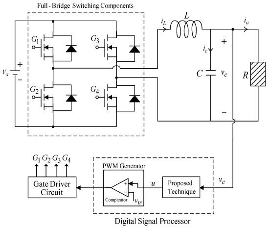
Figure 1.
Structure of DC–AC converter.
It can be seen from (1) and (2) that the error state equation of the DC–AC converter can be expressed as
where is the disturbance.
From (3), the control signal must be designed so well that the tracking error can converge to zero. In fact, the NTSMC is a fine control method with nonsingular fast convergence characteristics. The system (3) using NTSMC will achieve fast finite time convergence, strong robustness and infinite stability. However, when the load on a DC–AC converter is a large step change or uncertainty or even a severe nonlinear environment, a global optimization algorithm for the systematic and optimal choice of NTSMC parameter values is becoming more important. Based on such a motivation, and the practical application of artificial intelligence method is rapidly becoming a hot topic in engineering and science, it is a good idea to introduce an optimal methodology in the NTSMC design, providing an alternative reference for researchers. Therefore, NTSMC with BPSO method is proposed to improve the transience and steady-state behaviors of the classical TSMC to provide more accurate tracking. A DC–AC converter using this improved control design can produce a higher performance AC output voltage.
3. Proposed Control Technique
3.1. Problem Statement
First, a brief summary of the problem statement for a nonlinear system using the classical TSMC, is summarized and an improved technique is then designed. Consider the second-order uncertain nonlinear dynamic systems below:
where the system state is , and stands for a smooth nonlinear function , denotes parameter uncertainty and external disturbance and represents the control input.
To achieve finite time convergence of the system state, the following first-order terminal sliding variable can be defined as
where is the design constants and ( and are positive odd integers).
An SMC law , for , can be used, which is expressed as driving to the sliding mode for a limited time. Therefore, system dynamics can be controlled by the following differential equations:
The limited time from the initial state to zero can be determined by
This indicates the convergence of the two system states and the convergence of zero in a finite time in the NTSMC manifold. Considering the Jacobian matrix , the system state converges to zero gain in a finite time around the equilibrium .
From (8), we can obtain the eigenvalues of the first-order approximation matrix as follows.
It is inferred that the eigenvalue has a tendency of negative infinity at the equilibrium point, that is, the speed of the system trajectory to the equilibrium becomes infinite, resulting in limited time accessibility.
Thus, for error dynamics (3), the finite-time terminal sliding function can be expressed as
Using the (10), the and arrive within a limited time. The control law can be designed to ensure that TSM occurs as follows.
with
where , , , and called the equivalent control component, control undisturbed plants, such that and . The named sliding control component suppresses system uncertainty. Therefore, the state trajectory will reach the sliding mode and perform a limited system state convergence time. However, it is worth noting that there are the following problems in the equivalent control component: (i) If when and , the with may result in a singularity. This singularity causes the control law to produce an unbounded control signal, resulting in an unstable closed loop system. (ii) An imaginary number can be generated in a given situation .
3.2. Control Design
To overcome the singularity problem, the (10) is reconstructed into
where and , are positive odd numbers (). Then, a sliding-mode reaching equation is employed. The control law can be expressed as
with
where there is no negative index equivalent control , which results in non-singularity, and represents the sliding control for compensating the influence of the disturbance. Therefore, the system state will be forced to arrive and converge in a limited time.
Proof.
Choose Lyapunov candidate as
Along the dynamic system trajectory (3) and the control law (15), and use (14), the time derivative is given as
Since , , the surface of the NTSMC in (19) is allowed to converge to equilibrium in a limited time. Once , the state of system (3) will also converge to equilibrium within a finite time. However, the load may be a large load disturbance that provides inaccurate tracking performance in the system (3), i.e., the output voltage of the DC–AC converter is not exactly equal to the desired sinusoidal waveform. It is thus important to find out the optimal values of the NTSMC parameters in the (15) to maintain satisfactory performance of the DC–AC converter. To avoid tedious, time-consuming trial-and-error calculations, and obtain global best solutions, the BPSO method is employed to get the optimal value of NTSMC parameters. Finally, the combination of the DC–AC converter in (3) with BPSO method and NTSMC is asymptotically stable, and then achieves finite-time convergence to zero of tracking errors. The BPSO algorithm can be used illustrated in (20) and (21). The (20) and (21) show the evolution models of a particle. The speed and position of each particle can be renovated while flying toward aim.
where , and denote variables, and , indicate random numbers, is present flying speed, stands for present position, is local best position, represents global best position, and symbolizes sigmoid function that converts the particle velocity into the probability . □
4. Simulation and Experimental Results
In order to test the performance and robustness of the improved technique, the simulation and experimental results of the improved technique were compared to those obtained using the classical TSMC. The system parameters are as follows: The system parameter are listed as follows: , , , , , , , . Under the abrupt load change from no load to 12 ohm, the simulated results obtained using the improved technique and classical TSMC are shown in Figure 2 and Figure 3, respectively. Compared to classical TSMC, the improved technique exhibits a slight voltage drop and allows for fast output voltage recovery to verify its limited time accessibility. Due to the optimal tuning of the BPSO, after an instantaneous voltage dip (7 Vrms), the output voltage with the improved technique can be restored to the sinusoidal reference voltage, but the classical TSMC results in a large voltage dip (22 Vrms). Figure 4 shows that the improved technique can allow random variations in filter parameters L and C from 10% to 200% and 10% to 200% of the nominal value under a 12 ohm resistive load, respectively; however, the classical TSMC shown in Figure 5 yields the significant oscillations and leads to a descent in system robustness. Table 1 shows the simulated comparison of the voltage drop and %THD of the output voltage for step load and LC variation. A prototype of the DC–AC converter depicted as Figure 6 is constructed. Figure 7 illustrates the experimental waveform obtained using the improved technique under the step load from no load to 12 ohm at a 90 degree firing angle.
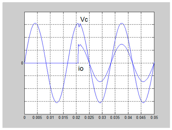
Figure 2.
Simulated waveforms under step load change (load suddenly turn on) for the improved technique (50 V/div; 10 A/div).
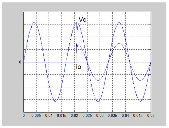
Figure 3.
Simulated waveforms under step load change (load suddenly turn on) for the classical TSMC (50 V/div; 10 A/div).
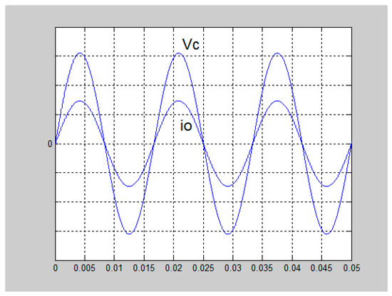
Figure 4.
Simulated waveform under LC (inductor capacitor) variation for the improved technique (50 V/div; 10 A/div).
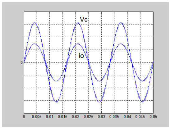
Figure 5.
Simulated waveforms under LC variation for the classical terminal sliding mode control (TSMC) (50 V/div; 10 A/div).

Table 1.
Simulated output-voltage slump and %THD under step loading and LC variation.
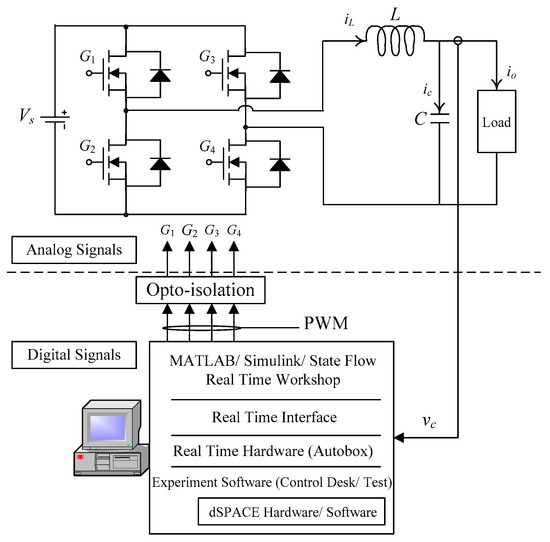
Figure 6.
Improved algorithm for DSP (digital signal processing)-based implementation.
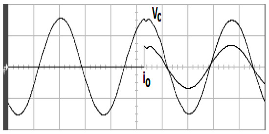
Figure 7.
Experimental waveforms under step loading from no load to full load with the improved technique (100 V/div; 20 A/div; 5 ms/div).
After the fast transient response with a voltage slump, the voltage waveform still keeps high tracking precision. Reversely, the experimental waveform obtained using the classical TSMC plotted in Figure 8 appears a large voltage slump and has a slow recovery time. In other words, the output voltage of the improved system due to the action of the BPSO can reach the 110 Vrms reference sine wave after the 8 Vrms small voltage slump, but the output-voltage slump with the classical TSMC is close to 36 Vrms, yielding an unsatisfactory performance in transience. The experimental system performance under the value of filter parameter (L and C) be assumed to undergo a random variation, i.e., 10% ~ 200% of nominal value at a 12 ohm resistive load, is investigated. As can be seen, the output-voltage of the Figure 9 obtained using the improved technique provides the robust ability of greater parameter variation tolerance. However, it is worth noting that a long-time distortion with the sensitivity at the beginning of the waveform exists in the output-voltage with the classical TSMC as shown in Figure 10. Table 2 lists the experimental output-voltage slump and THD values under step load and LC variation.
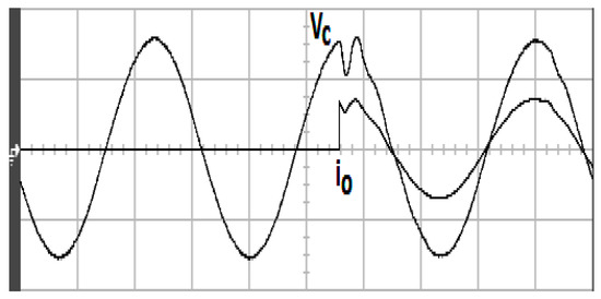
Figure 8.
Experimental waveforms under step loading from no load to full load with the classical TSMC (100 V/div; 20 A/div; 5 ms/div).
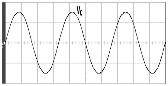
Figure 9.
Experimental output-voltage under LC variation with the improved technique (100 V/div; 5 ms/div).
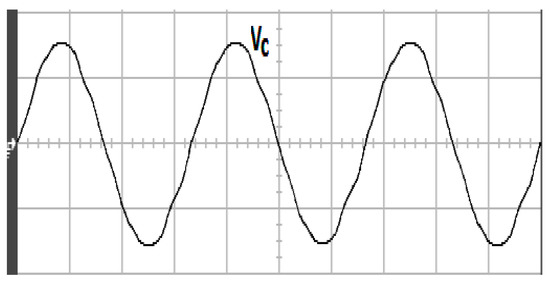
Figure 10.
Experimental output-voltage under LC variation with the classical TSMC (100 V/div; 5 ms/div).
Table 2.
Experimental output-voltage slump and %THD under step loading and LC variation.
5. Discussion and Future Research
The improved technique has been proposed for reducing jitter, steady-state error attenuation and greater interference rejection resulting in good system performance. However, in order to advance future research, we have reviewed a large amount of literature on sliding modes, especially in high-order SMC (HOSMC) and adaptive SMC [30,31,32,33,38]. The adaptive SMC not only reduces the jitter and steady-state error but also avoids nominal knowledge requirement of the system. The HOSMC method [44,45] reported on a topic of recent interest in SMC theory. For example, in the th-order HOSMC, the derivative of the th control input becomes continuous, and both the sliding plane and its high-order derivative need to be zero. Therefore, the HOSMC retains the original features of the traditional SMC while producing less jitter and better convergence accuracy. The HOSMC method has been used to control DC–AC converter related systems [46,47,48,49]. The grid-connected wind energy conversion system is designed by multiple input multiple output HOSMC, so it can adjust active and reactive power, and even develop a switching control scheme based on voltage grid measurement. This approach yields attractive benefits such as robust robustness to system uncertainty, reduced jitter, and finite time convergence of system states to sliding surfaces [46]. A reverse-threshold HOSMC strategy is proposed for grid-connected distributed generation (DG) units. It provides excellent regulation of the inverter output current and provides a perfect sinusoidal balanced current for the grid, resulting in a distributed generator system with good performance against model uncertainties, parameter variations and unmodeled dynamics as well as external disturbances [47]. HOSM observers are effectively introduced into the control design of single-phase DC–AC inverter systems to suppress multiple sources of interference/uncertainty, including parametric perturbations, complex nonlinear dynamics, and external disturbances. Based on the Lyapunov function criterion, the stability of the whole system and the effectiveness of the high-order sliding mode observer are rigorously proved [48]. In addition, an improved HOSM observer is proposed for use in a proton exchange membrane fuel cell system based on excess oxygen ratio, which provides an observation of unmeasurable system conditions. Even under the influence of measurement noise, modeling error, parameter uncertainty and strong external interference, the method still has good robustness and fast convergence, and has limited time stability [49]. As mentioned above, HOSMC produces high-order derivative constraints on the sliding surface while preserving the main advantages of traditional SMC; it is undeniable that HOSMC eliminates jitter effects and produces more accurate control performance. Therefore, HOSMC will promote further research in this area of the DC–AC converter.
6. Conclusions
In this paper, a BPSO optimized NTSMC for a DC–AC converter is described that is capable of producing low THD and fast transients. The importance of the NTSMC is limited system state convergence time and no singularities. Also, the parameters of the NTSMC should be chosen well to obtain optimal performance. These parameters are traditionally determined by a trial and error method, which is very tedious, laborious to implement, and time-consuming. Therefore, the BPSO is used to optimize the NTSMC parameters, yielding better transient and steady-state response. The Lyapunov method is used to analyze the stability of the improved technique. The finite time accessibility of the sliding surface, the asymptotic stability of the closed-loop system and the finite time convergence of the tracking error are proved. Therefore, we believe that the improved technique will contribute to the control design of future artificial intelligence related systems. Simulations and experiments have been developed on prototypes of DC–AC converters using DSP to verify the applicability of the improved technique.
Author Contributions
E.-C.C. conceived, investigated and designed the circuit, and developed the methodology. C.-A.C. and L.-S.Y. prepared software resources, set up simulation software, and E.-C.C. performed circuit simulations. E.-C.C. carried out DC–AC converter prototype, and measured as well as analyzed experimental results. E.-C.C. wrote the paper and revised it for submission.
Funding
This research was funded by the Ministry of Science and Technology (MOST) of Taiwan, R.O.C., under contract MOST 107-2221-E-214-006.
Acknowledgments
The authors gratefully acknowledge the financial support of the Ministry of Science and Technology of Taiwan, R.O.C., under project number MOST 107-2221-E-214-006.
Conflicts of Interest
The authors declare no conflicts of interest regarding the publication of this article.
References
- Jeyraj, S.; Rahim, N.A. Multilevel inverter for grid-connected PV system employing digital PI controller. IEEE Trans. Ind. Electron. 2009, 56, 149–158. [Google Scholar]
- Mirzaei, M.; Tibaldi, C.; Hansen, M.H. PI controller design of a wind turbine: Evaluation of the pole-placement method and tuning using constrained optimization. J. Phys. Conf. Ser. 2016, 753, 1–7. [Google Scholar] [CrossRef]
- Jin, W.; Li, Y.L.; Sun, G.Y.; Bu, L.Z. H-infinity repetitive control based on active damping with reduced computation delay for LCL-type grid-connected inverters. Energies 2017, 10, 586. [Google Scholar]
- Xie, C.; Zhao, X.; Savaghebi, M.; Meng, L.; Guerrero, J.M.; Quintero, J.C.V. Multirate fractional-order repetitive control of shunt active power filter suitable for microgrid applications. IEEE J. Emerg. Sel. Top. Power Electron. 2017, 5, 809–819. [Google Scholar] [CrossRef]
- Benyoucef, A.; Kara, K.; Chouder, A.; Silvestre, S. Prediction-based deadbeat control for grid-connected inverter with L-filter and LCL-filter. Electr. Power Compon. Syst. 2014, 42, 1266–1277. [Google Scholar] [CrossRef]
- Kim, J.; Hong, J.; Kim, H. Improved direct deadbeat voltage control with an actively damped inductor-capacitor plant model in an islanded AC microgrid. Energies 2016, 42, 978. [Google Scholar] [CrossRef]
- Bevrani, H.; Feizi, M.R. Robust frequency control in an islanded microgrid: H-infinity and mu-synthesis Approaches. IEEE Trans. Smart Grid 2016, 7, 706–717. [Google Scholar] [CrossRef]
- Ren, F.Y.; Lin, C.; Yin, X.H. Design a congestion controller based on sliding mode variable structure control. Comput. Commun. 2005, 28, 1050–1061. [Google Scholar] [CrossRef]
- Ignaciuk, P.; Bartoszewicz, A. Congestion Control in Data Transmission Networks: Sliding Mode and Other Designs (Communications and Control Engineering); Springer: New York, NY, USA, 2013. [Google Scholar]
- Tan, S.C.; Lai, Y.M.; Tse, C.K. Sliding Mode Control of Switching Power Converters: Techniques and Implementation; Taylor & Francis: Boca Raton, FL, USA, 2012. [Google Scholar]
- Yu, X.; Kaynak, O. Sliding mode control with soft computing: A survey. IEEE Trans. Ind. Electron. 2009, 56, 3275–3285. [Google Scholar]
- Kang, S.W.; Kim, K.H. Sliding mode harmonic compensation strategy for power quality improvement of a grid-connected inverter under distorted grid condition. IET Power Electron. 2015, 8, 1461–1472. [Google Scholar] [CrossRef]
- Kaynak, A.B.; Utkin, V.I. Industrial applications of sliding mode: Control Part II. IEEE Trans. Ind. Electron. 2009, 56, 3271–3274. [Google Scholar] [CrossRef]
- Kayacan, E.; Cigdem, O.; Kaynak, O. Sliding mode control approach for online learning as applied to type-2 fuzzy neural networks and its experimental evaluation. IEEE Trans. Ind. Electron. 2012, 59, 3510–3520. [Google Scholar] [CrossRef]
- Vardan, M.; Ekaterina, A. Sliding Mode in Intellectual Control and Communication: Emerging Research and Opportunities; IGI Global: Hershey, PA, USA, 2017. [Google Scholar]
- Derbel, N.; Ghommam, J.; Zhu, Q.M. Applications of Sliding Mode Control; Springer: Singapore, 2017. [Google Scholar]
- Yan, X.G.; Spurgeon, S.K.; Edwards, C. Variable Structure Control of Complex Systems: Analysis and Design; Springer International Publishing: New York, NY, USA, 2017. [Google Scholar]
- Andreas, R.; Luise, S. Variable-Structure Approaches: Analysis, Simulation, Robust Control and Estimation of Uncertain Dynamic Processes; Springer International Publishing: New York, NY, USA, 2016. [Google Scholar]
- Abrishamifar, A.; Ahmad, A.A.; Mohamadian, M. Fixed switching frequency sliding mode control for single-phase unipolar inverters. IEEE Trans. Power Electron. 2012, 27, 2507–2514. [Google Scholar] [CrossRef]
- Hao, X.; Yang, X.; Liu, T.; Huang, L.; Chen, W.J. A sliding-mode controller with multiresonant sliding surface for single-phase grid-connected VSI with an LCL filter. IEEE Trans. Power Electron. 2013, 28, 2259–2268. [Google Scholar] [CrossRef]
- Aghatehrani, R.; Kavasseri, R. Sensitivity-analysis-based sliding mode control for voltage regulation in microgrids. IEEE Trans. Sustain. Energy 2013, 4, 50–57. [Google Scholar] [CrossRef]
- Camila, L.C.; Tiago, R.O.; Jose, P.V.S.C. Output-feedback sliding-mode control of multivariable systems with uncertain time-varying state delays and unmatched non-linearities. IET Control Theory Appl. 2013, 7, 1616–1623. [Google Scholar]
- Hung, L.C.; Lin, H.P.; Chung, H.Y. Design of self-tuning fuzzy sliding mode control for TORA system. Expert Syst. Appl. 2007, 32, 201–212. [Google Scholar] [CrossRef]
- Hemdani, A.; Dagbagi, M.; Naouar, W.M.; Idkhajine, L.; Belkhodja, I.S.; Monmasson, E. Indirect sliding mode power control for three phase grid connected power converter. IET Power Electron. 2015, 8, 977–985. [Google Scholar] [CrossRef]
- Liu, J.K.; Wang, X.H. Terminal Sliding Mode Control. In Advanced Sliding Mode Control for Mechanical Systems; Springer: Berlin, Germany, 2011; pp. 137–162. [Google Scholar]
- Bhave, M.; Janardhanan, S.; Dewan, L. A finite-time convergent sliding mode control for rigid underactuated robotic manipulator. Syst. Sci. Control Eng. 2014, 2, 493–499. [Google Scholar] [CrossRef]
- Hong, Y.G.; Yang, G.W.; Cheng, D.Z.; Spurgeon, S. Finite time convergent control using terminal sliding mode. J. Control Theory Appl. 2004, 2, 69–74. [Google Scholar] [CrossRef]
- Yu, X.H.; Xu, J.X. Variable Structure Systems with Terminal Sliding Modes. In Variable Structure Systems: Towards the 21st Century; Springer: Berlin, Germany, 2002. [Google Scholar]
- Roy, S.; Roy, S.B.; Kar, I.N. Adaptive–robust control of euler–lagrange systems with linearly parametrizable uncertainty bound. IEEE Trans. Control Syst. Technol. 2018, 26, 1842–1850. [Google Scholar] [CrossRef]
- Roy, S.; Roy, S.B.; Kar, I.N. A new design methodology of adaptive sliding mode control for a class of nonlinear systems with state dependent uncertainty bound. In Proceedings of the 2018 15th International Workshop on Variable Structure Systems (VSS), Graz, Austria, 9–11 July 2018; pp. 414–419. [Google Scholar]
- Roy, S.; Kar, I.N. Adaptive-robust control of uncertain euler-lagrange systems with past data: A time-delayed approach. In Proceedings of the 2016 IEEE International Conference on Robotics and Automation (ICRA), Stockholm, Sweden, 16–21 May 2016; pp. 5715–5720. [Google Scholar]
- Roy, S.; Kar, I.N.; Lee, J.; Tsagarakis, N.G.; Caldwell, D.G. Adaptive-robust control of a class of el systems with parametric variations using artificially delayed input and position feedback. IEEE Trans. Control Syst. Technol. 2019, 27, 603–615. [Google Scholar] [CrossRef]
- Roy, S.; Kar, I.N.; Lee, J.; Jin, M.L. Adaptive-robust time-delay control for a class of uncertain euler–lagrange systems. IEEE Trans. Ind. Electron. 2017, 64, 7109–7119. [Google Scholar] [CrossRef]
- Plestan, F.; Shtessel, Y.; Brégeault, V.; Poznyak, A. Sliding mode control with gain adaptation—Application to an electropneumatic actuator. Control Eng. Pract. 2013, 21, 679–688. [Google Scholar] [CrossRef]
- Plestan, F.; Shtessel, Y.; Brégeault, V.; Poznyak, A. New methodologies for adaptive sliding mode control. Int. J. Control 2010, 83, 1907–1919. [Google Scholar] [CrossRef]
- Utkin, V.I.; Poznyak, A.S. Adaptive sliding mode control with application to super-twist algorithm: Equivalent control method. Automatica 2013, 49, 39–47. [Google Scholar] [CrossRef]
- Moreno, J.A.; Negrete, D.Y.; González, V.T.; Fridman, L. Adaptive continuous twisting algorithm. Int. J. Control 2016, 89, 1798–1806. [Google Scholar] [CrossRef]
- Roy, S.; Lee, J.N.; Baldi, S. A New Continuous-Time Stability Perspective of Time-Delay Control: Introducing a State-Dependent Upper Bound Structure. IEEE Control Syst. Lett. 2019, 3, 475–480. [Google Scholar] [CrossRef]
- Alireza, S.; Mozhgan, A. Binary PSO-based dynamic multi-objective model for distributed generation planning under uncertainty. IET Renew. Power Gener. 2012, 6, 67–78. [Google Scholar]
- Lin, C.J.; Chern, M.S.; Chih, M.C. A binary particle swarm optimization based on the surrogate information with proportional acceleration coefficients for the 0-1 multidimensional knapsack problem. J. Ind. Prod. Eng. 2016, 33, 77–102. [Google Scholar] [CrossRef]
- Silva, S.A.; Sampaio, L.P.; Oliveira, F.M.; Durand, F.R. Feed-forward DC-bus control loop applied to a single-phase grid-connected PV system operating with PSO-based MPPT technique and active power-line conditioning. IET Proc. Renew. Power Gener. 2017, 11, 183–193. [Google Scholar] [CrossRef]
- Babu, T.S.; Ram, J.P.; Dragicevic, T.; Miyatake, M.; Blaabjerg, F.; Rajasekar, N. Particle Swarm Optimization Based Solar PV Array Reconfiguration of the Maximum Power Extraction Under Partial Shading Conditions. IEEE Trans. Sustain. Energy 2018, 9, 74–85. [Google Scholar] [CrossRef]
- Awadallah, M.A.; Venkatesh, B. Bacterial Foraging Algorithm Guided by Particle Swarm Optimization for Parameter Identification of Photovoltaic Modules. Can. J. Electr. Comput. Eng. 2016, 39, 150–157. [Google Scholar] [CrossRef]
- Emel’yanov, S.V.; Korovin, S.K.; Levant, A. High order sliding modes in control systems. Comput. Math. Model. 1996, 7, 294–318. [Google Scholar]
- Levant, A. Higher-order sliding modes, differentiation and output-feedback control. Int. J. Control 2003, 76, 924–941. [Google Scholar] [CrossRef]
- Valenciaga, F.; Fernandez, R.D. Multiple-input–multiple-output high-order sliding mode control for a permanent magnet synchronous generator wind-based system with grid support capabilities. IET Renew. Power Gener. 2015, 9, 925–934. [Google Scholar] [CrossRef]
- Dehkordi, N.M.; Sadati, N.; Hamzeh, M. A robust backstepping high-order sliding mode control strategy for grid-connected DG units with harmonic/interharmonic current compensation capability. IEEE Trans. Sustain. Energy 2017, 8, 561–572. [Google Scholar] [CrossRef]
- Chen, D.; Jun, Y.; Wang, Z.; Li, S.H. Universal active disturbance rejection control for non-linear systems with multiple disturbances via a high-order sliding mode observer. IET Control Theory Appl. 2017, 11, 1194–1204. [Google Scholar]
- Deng, H.W.; Li, Q.; Chen, W.R.; Zhang, G.R. High-order sliding mode observer based OER control for PEM fuel cell air-feed system. IEEE Trans. Energy Convers. 2018, 33, 232–244. [Google Scholar] [CrossRef]


© 2019 by the authors. Licensee MDPI, Basel, Switzerland. This article is an open access article distributed under the terms and conditions of the Creative Commons Attribution (CC BY) license (http://creativecommons.org/licenses/by/4.0/).