Optimization of Safety Stock under Controllable Production Rate and Energy Consumption in an Automated Smart Production Management

Abstract

A smart production system is essential to produce complex products under the consumption of efficient energy. The main ramification of controllable production rate, amount of production size, and safety stocks is simultaneously optimized under proper utilization of energy within a smart production system with a random breakdown of spare parts. Due to the random breakdown, a greater amount of energy may be used. For this purpose, this study is concerned about the optimum safety stock level under the exact amount of energy utilization. For random breakdown, there are three cases as production inventory meets the demand without utilization of the safety stock, with using of the safety stock, and consumed the total safety stock amount and facing shortages. After the random breakdown time, the smart production system may move to an out-of-control state and may produce defective items, where the production rate of defective items is a random variable, which follows an exponential distribution. The total cost is highly nonlinear and cannot be solved by any classical optimization technique. A mathematical optimization tool is utilized to test the model. Numerical study proves that the effect of energy plays an important role for the smart manufacturing system even though random breakdowns are there. it is found that the controllable production rate under the effect of the optimum energy consumption really effects significantly in the minimization cost. It saves cost regarding the corrective and preventive maintenance cost. The amount of safety stock can have more support under the effect of optimum energy utilization. The energy can be replaced by the solar energy.

1. Introduction

Recently, the main development in the production sector is the inspection of smart manufacturing within the production context. The effect of energy is another critical milestone for the smart manufacturing system (see for reference Sarkar et al. [1]). C$\acute{\mathrm{a}}$rdenas-Barr$\acute{\mathrm{o}}$n [2] introduced an optimum production strategy for those products, which have special property like as fixed lifetime but that model did not consider the machine breakdown during making the production policies. Thus, there was no assumption for using the extra energies during machine breakdown and how to reduce those energies by using renewable energy. This proposed model would like to consider this research gap within the literature to obtain the minimum total cost for the smart production system. Talizadeh et al. [3] introduced the outsourcing reworked strategy for defective products within a traditional production system, but there is not a single assumption regarding energy reduction or uses of renewable energy. That research gap is also fulfilled by this proposed research. Wee et al. [4] introduced renewable energy within the supply chain management for the performance, limitations for their uses, and further improvement for different policies. But, there is no indication how to transfer non-renewable to renewable energy within a smart production system. Therefore, this study introduces the strategy for reduced energy consumption through renewable energy resources.

The main aim of this smart production is to make a controllable production for making more smart products than the existing one and to reduce human labor’s efforts. But the main difference between an additive manufacturing and a smart manufacturing is that the additive manufacturing prefers more machinery controls than human labor, whereas the main theme of smart manufacturing systems is to make a human-factor related complex controllable management such that human-machine interactions can be used in the proper way to obtain the best complex products Kang et al. ([5]) through skilled nature of labors. Kang et al. [5] proved that the human interaction system must be controlled by a smart manufacturing system where the main performance of inspection is conducted by the three specified labors like skilled, unskilled, and semi-skilled labors. But the main issue is that they did not consider anything in the direction of energy. However, in any smart manufacturing system, the main base is smart machines and human labors and the interactions between them. Within the smart production system, there are two policies for breakdown case as no-resumption (NR) and abort/resume (AR). NR means the production may start again after repair of defective machine provided all inventories are utilized and AR means the production will start just after the repair of breakdown machine with the condition that the existing inventory should deplete to a certain amount of safety stock. Therefore, to maintain the breakdown of the system, the preventive and corrective maintenance are used. Even though both the maintenance are used, the inventory can touch the zero level without facing shortages, it may happen that inventory can go below the zero level but, it still lies in between zero and safety stock level, or sometimes it may happen that the inventory may reach to the downside of the safety stock and facing the shortages. Therefore, it can be understood that the safety stock plays an important role, whose decision is generally taken by the management sector of the smart manufacturing system. Porteus [6] first introduced the concept of improvement for the production system’s quality and reduction of setup cost by using some investments. Khouja and Mehraj [7] first introduced the controllable production rate, where the production rate is variable within a certain interval of production capacity. They used that the unit production cost is dependent on a variable production rate. This is the basic idea for the controllable production rate within a traditional production model, which is the major turning of the smart production without having any consideration of energy consumption. Chung and Hou [8] extended the basic production model Khouja and Mehraj [7] with shortages, imperfect production, and the elapsed time duration of the process distribution without anything related with energy. Giri and Dohi [9] first introduced the random breakdown within a production context, where the production lot size is a decision variable and the failure rate is considered as random exponential distribution. Avancini et al. [10] defined several matrices for energy evaluation in any smart system. They explained how the intelligent network supports for energy efficiency but there is a lack of specification any production system. Because, each production system is different with each other for the purpose of energy consumption issue. They just described about the control, communication, and display with the efficient energy. Chen and Lo [11] developed warranty policy for defective products in an imperfect production system where shortages appear due to random defective products. Even though the defective products are produced, there is no concept of the optimum energy consumption. Nižetić et al. [12] introduced several smart technologies to manage wastes through the efficient energies. They used sustainable resources to reduce the global energy but it has lack of concept within the smart production system. Specifically, the effect of efficient energy was not considered by any researcher yet. An economic production model for imperfect production system was developed by Sarkar and Moon [13]. They considered defective products when the system moves to out-of-control state from the in-control state. They did not consider any type of preventive or corrective maintenance. They just considered a traditional production system with out-of-control movement without any concept of energy. A two-echelon supply chain management is explained with probabilistic deterioriation in Sarkar [14]. The aim of the supply chain is to reduce the total cost but with a traditional production system. Any energy consumption is not considered within the whole supply chain model. For any smart production system, smart optimum energy and finally smart optimum energy system are very much essential to make any grid system with the help of grid system, the smart machine can be worked properly within several smart production systems, but Lund et al. [15] described only the explanation of grid system without modelling any specific smart production system. Generally, the smart manufacturing utilizes smart integrating intelligent manufacturing machines to produce smart products. The process is totally controlled though automated machines Edgar and Pistikopoulos [16]. Sana et al. [17] discussed that those defective products can be sold by reduced price. However, none of the authors did consider energy consumption in any production context. Louly and Dolgui [18] derived the optimum safety stock level in an assembly production system but without any concept of energy. Jaber et al. [19] were the pioneer researcher about the incorporation the entropy/heat effect in any inventory model but no energy effect. Sarkar et al. [20] explained the joint effect of failure rate, safety stock, and production lot in a basic production mode under a corrective maintenance and preventive maintenance. They proved that safety stock production model converges always over the non-safety stock mode but without any concept of energy or heat effect. Sana [21] developed a production model with machine breakdown under both types of maintenance where the shifting mode for machine follows an exponential distribution. Sarkar et al. [22] developed a closed-loop supply chain model with environmental issues. In this model remanufacturing of returned products are considered. But, any energy issue were not take into consideration. A supply chain model for complementary products was proposed by Sarkar et al. [23] without any energy effect, but the variable production rate and time dependent holding costs are applied. A logistic model was developed by Sarkar et al. [24], where the optimal cash flow for a smart production system is described. In this model carbon foot print and carbon emission costs were considered witout any energy consideration. C$\acute{\mathrm{a}}$rdenas-Barr$\acute{\mathrm{o}}$n et al. [25] developed the benefit of multi-shipment in an economic manufacturing model without having any concept of energy matter. Giotitsa et al. [26] strives an appropriate approach for production of energy and its distribution. Tayyab and Sarkar [27] were the pioneer about incorpration random backorder rate within a multi-stage production system. Omair and Sarkar [28] introduced some sustainability issues within the production context without having any concept of energy consideration. Kim and Sarkar [29] explained a multi-stage cleaner production model, but they did not consider any idea about renewable energy effect within the multi-stage production system. They consider production system moves to out-of-control state even though they did not consider machine breakdown only, they just assumed the production system moves out-of-control state from in-control state due to labor strickes and machine breakdown without calculating breakdowns within inventory calculation. In this same direction, Moon et al. [30] approached a continous review model with service level and variable lead time without any smart production consideration. A two-echelon supply chain model with quality improvement and setup cost reduction in a tradition production system was considered by Sarkar et al. [31], but production rate is constant though it moves to out-of-control state. A supply chain model Kim and Sarkar [32] was developed with stochastic lead time and transportation discount policy without any maintainence policy. A study on setup cost reduction and quality improvement of manufacturing system was proposed by Majumder et al. [33] within a traditional production system. For an imprfect production system, lost sales reduction and quality improvement was taken account in fuzzy environment by Soni et al. [34], but still they did not think about the smart production system. Sarkar et al. [35] explained about a two-echelon supply chain model with setup time reduction and effect of safety factor in a traditional system. An integrated inventory model was developed by Dey et al. [36] on variable safety fctor and setup cost reduction. But for all of these models, maintainenece costs along with the energy costs are not considered for any stage of the supply chain or the production. Sarkar et al. [37] explained only out-of-control machines but did not consider the breakdown effects on the inventory of the production system. Biel and Glock [38] discussed an efficient way to use waste energy within a two-stage controllable production system. Kim et al. [39] developed a cleaner multi-stage production system with a random backorder rate without any sustainable issue or energy issue. Unver and Kara [40] developed the efficiency of energy consumption within a traditional process with the optimum energy consumption. They did not consider any maintenance or any controllable smart production system. Kumar et al. [41] maintained the efficient balance level within a production system. They calculated the amount of wastes in a downstream production system and they obtained several strategies to reduce those wastes. Morato et al. [42] did the reverse way of energy issue. They calculated the amount of energy during the production system for the agricultural products. Ahmed and Sarkar [43] introduced sustainable framework and an energy issue for the case of biofuel production. Darom et al. [44] developed two serial supply chain disruption recoveries with controlled safety-stock and constant production rate. Assid et al. [45] introduced an unreliable hybrid manufacturing for production and setup cost controlling. They used demand of new and remanufacturing products, which are reworked but they did not mention the time of rework. [46] introduced an unique way to decide the exact time of rework within a multi-stage single cycle and multi-stage multi-cycle production system even though Sarkar [46] did not take into account of energy cost and any controllable production system. Utilizing photovoltaic technology, the optimum amount of energy consumption within a production buffer stock was developed by Caro-Ruiz et al. [47]. They proved that the coordination is possible for production system with a energy factory with the optimum consumption. Finally, one can obtain the idea about the automation policy in a smart production system, where machinery systems are automatic and they are controlled by several automated system of energy (Dincer and Ezzat [48], Dincer and Al-Zareer [49], Dincer and Rosen [50], Dincer and Rosen [51], and Dincer and Bicer [52]). However, if the automated system is utilized in several research models (Lu et al. [53], Kazemi et al. [54], Kulczek [55], Harris et al. [56], Bruni et al. [57], Dehning et al. [58], and Nordborg et al. [59]), the optimum renewable energy under production maintenance is not considered. The main research gap regarding maintenance is not considered as it was assumed that smart production system always gives perfect smart products without any breakdown and without any maintenance ( Khalil et al. [60], Keen et al. [61], Chen et al. [62], and Liang et al. [63]).

Still, there is a research gap in the direction of smart production direction with random breakdown under the proper application of corrective and preventive maintenance where the main task is to control used energy within the smart production system. This proposed model has solved this research gap for this matter. The

Table 1. Research contribution by several authors.

Author(s)	Energy	Smart Production System	Breakdown	Safety Stock	Production Rate	Maintenance
Sarkar et al. [1]	Consumption	Smart	Random	NA	Variable	NA
Kang et al. [2]	NA	Smart	NA	NA	Constant	NA
Porteus [3]	NA	Traditional	NA	NA	Constant	NA
Khouja and Mehraj [4]	NA	Traditional	NA	NA	Variable	NA
Giri and Dohi [6]	NA	Traditinal	Random	NA	Constant	CM and PM
Chenand Lo [7]	NA	Traditional	NA	NA	Constant	NA
Sana et al. [8]	NA	Traditional	Random	NA	Constant	CM and PM
Louly and Dolgui [9]	NA	Traditional	NA	Variable	Constant	CM and PM
Sarkar et al. [11]	NA	Traditional	Random	Variable	Constant	CM and PM
This paper	Consumption	Smart	Random	Variable	Variable	CM and PM

NA indicates that is not applicable for that paper. CM and PM stand for corrective and preventive maintenance, respectively.

shows the research gaps of the model.

2. Problem Definition, Notation, and Assumptions

In this section, problem definition, assumptions and notation are given.

2.1. Problem Definition

It is a smart production system, random breakdown and defective production exists under controllable energy consumption and production rate, then how safety stock can be maintained within the production with the minimum cost. The unit production cost is dependent on controllable production rate and efficient amount of energy. Due to the random breakdown, the corrective and preservative maintenance are considered. As random breakdown is an unusual event and similarly amount of energy is used as extra amount of energy during corrective maintenance of smart machines. There are several cases, where the existing inventory’s position is before safety stock or after safety stock amount. The controllable production rate must vary within proper limit of production capacity of the machines such that the optimum amount of energy can be used. Finally, the aim is to minimize the optimum cost under the optimum production lot, safety stock and the production rate.

2.2. Assumptions

The following assumptions are considered to develop this model.

• A smart production management is considered for single-type of products production under a controllable production rate and the optimum energy consumption.
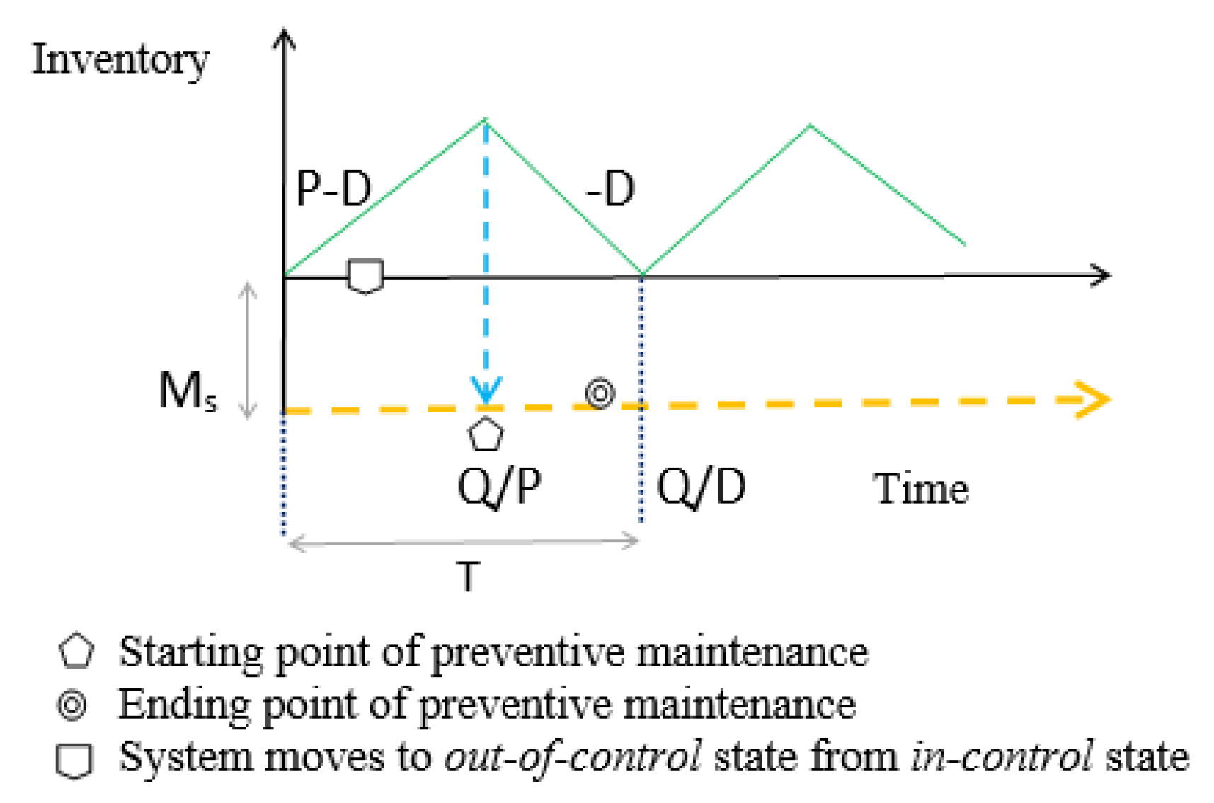
• During a long-run production system, the random breakdown may occur. Based on it, the model considers three cases as (i) the inventory just reaches to zero but no shortage appears (ii) the inventory may exceed the zero axis level but less than the safety stock level (iii) the inventory may cross the safety stock level and faces shortages.
• Regular and emergency maintenance are considered under the effect of energy with two specified probability distribution functions.
• Random breakdown may be at a random time, which follows an exponential distribution.
• The effect of energy is considered for all possible position with the optimum amount of energy consumption.
• Safety stock, production rate, and production quality are considered as decision variable where production rate may vary within the range of $[p_{min},p_{max}]$. The optimum value of production rate must lie within the interval.
• Shortages appear if the inventory crosses the safety stock level. If shortages appear, it is considered fully backordered.

2.3. Notation

Table 2. Notation for parameters and variables.

Decision variables
P	production rate (units/time)
Q	production lot size (units)
$M_s$	safety stock (units)
Random variable
$\rho$	random variable of shifting from in-control-state to an out-of-control state
Parameters
D	demand rate (units)
X	non-negative random variable denoting time
$F_X$$\left(t\right)$	failure time-distribution of X with probability density function $f_X$ $\left(t\right)$ = ${\displaystyle \frac{d}{dt}}$ $\left(F_X\left(t\right)\right)$
$A_1$$\left(S_1\right)$	corrective(emergency) repair time distribution with probability density function $a_1$
	($S_1$) with finite mean ${\displaystyle \frac{1}{{\mu }_1}}$( > 0)
$A_2$$\left(S_2\right)$	preventive(regular) repair time distribution with probability density function $a_2$
	($S_2$) with finite mean ${\displaystyle \frac{1}{{\mu }_2}}$( > 0)
$A_0$	setup cost per setup for the smart manufacturing system
$A_0^{\prime }$	energy cost for setup the production system
$C_{CRC}$	corrective repair cost per unit time
$C_{CRC}^{\prime }$	energy cost for corrective maintenance per unit time
$C_{PRC}$	preventive repair cost per unit time
$C_{PRC}^{\prime }$	preventive maintenance energy cost per unit time
$C_{hold}$	holding cost per unit per unit time
$C_{hold}^{\prime }$	energy cost to hold all products per unit per unit time
$C_{shor}$	shortage cost per unit product
$C_{re}$	rework cost per unit of defective item
$C_{re}^{\prime }$	energy cost per unit to rework defective items
$h\left(\rho \right)$	probability distribution function of the shift time distribution
$\beta$	proportion of defective items produced in the out-of control state where $0<\beta <1$
T	cycle length of production-inventory system

represents the notation of this model.

3. Mathematical Model

A basic smart production is taken to produce a single-type of smart products. Even though, it is a smart production system, the machine failure exists and defective products produced. During long-run, the smart production system may move to out-of-control state from in-control state due to semi-skilled laborer’s issues or machinery problems. The smart production begins to produce smart products at time $t=0$ with a controllable production rate $\rho$ and continues until the time $t_1$, when the inventory touches the maximum holding if there does not exist any smart machine breakdown. But the random breakdown occurs within this smart production system. Due to the random breakdown there are some possibilities like the preventive or corrective maintenance’s time with efficient energy is less than or greater than expected time. Thus, shortages may occur. The following cases under efficient time can be founded as follows:

Case I: Inventory position due to preventive maintenance

If the preventive maintenance time under the efficient energy is less than or equal to ${\displaystyle \frac{Q(P-D)}{PD}}$, then amount of inventory is (see Figure 1)

$$\begin{array}{ccc}\hfill I_1& =& {\int }_0^{Q(P-D)/\left(PD\right)}\left[{\displaystyle \frac{(P-D)Q^2}{2PD}}+{\displaystyle \frac{M_{s}Q}{D}}\right]d{A}_1\left(S_1\right).\hfill \end{array}$$

(1)

But, if the preventive maintenance time belongs to $\left[{\displaystyle \frac{Q(P-D)}{PD}},{\displaystyle \frac{(M_s+{\displaystyle \frac{Q(P-D)}{P}})}{D}}\right]$, then the inventory may reach lower than the safety stock level but still there is no shortage as the inventory level is above the zero level, then the amount of inventory is (refer to Figure 2)

$$\begin{array}{ccc}\hfill I_2& =& {\int }_{Q(P-D)/\left(PD\right)}^{(M_s+Q(P-D)/P)/D}\left[{\displaystyle \frac{(P-D)Q^2}{2PD}}+{\displaystyle \frac{P{M}_s{S}_1}{(P-D)}}-{\displaystyle \frac{P{(S_{1}D-(P-D)Q/P)}^2}{2D(P-D)}}\right]d{A}_1\left(S_1\right).\hfill \end{array}$$

(2)

Finally, if the preventive maintenance time belongs to $\left[{\displaystyle \frac{(M_s+{\displaystyle \frac{Q(P-D)}{P}})}{D}},\infty \right)$, then the shortage arises due to the inventory level reaches below the zero level, then the total amount of inventory is (see Figure 3)

$$\begin{array}{ccc}\hfill I_3& =& {\int }_{(M_s+Q(P-D)/P)/D}^{\infty }\left[{\displaystyle \frac{(P-D)Q^2}{2PD}}+{\displaystyle \frac{M_{s}Q}{P}}+{\displaystyle \frac{P{M}_s^2}{2D(P-D)}})\right]d{A}_s\left(S_1\right),\hfill \end{array}$$

(3)

and the inventory due to shortage for the preventive maintenance is

$$\begin{array}{c}\hfill I_4={\int }_{(M_s+Q(P-D)/P)/D}^{\infty }\left[S_1-(M_s+Q(P-D)/P)/D\right]d{A}_s\left(S_1\right).\end{array}$$

(4)

Now, the inventory related with corrected maintenance can be done in case II.

Case II: Inventory position due to the corrective maintenance

The corrective maintenance is conducted when there in any urgent mishap and to save the production system, it is needed to maintenance with cost and more energy investment. Thus, one can calculate the amount of inventory position based on random time t for corrective maintenance as at random time $t=\rho$, the process moves to out-of-control state from in-control state. Similar of Case I, there are three cases when the corrective maintenance time belongs to $\left[0,{\displaystyle \frac{t(P-D)}{D}}\right]$, the inventory position is within the general range of inventory above zero level, or the maintenance time belongs to $\left[{\displaystyle \frac{t(P-D)}{D}},{\displaystyle \frac{(M_s+t(P-D))}{D}}\right]$, the position of inventory should lie in between zero level and safety stock level without having shortages, but if the time for maintenance belongs to $\left[{\displaystyle \frac{(M_s+t(P-D))}{D}},\infty \right)$, then inventory level reaches below the safety stock level, with having shortages, then the inventory positions, respectively are (see Figure 4, Figure 5 and Figure 6)

$$\begin{array}{ccc}\hfill I_5& =& {\int }_0^{t(P-D)/D}\left[{\displaystyle \frac{(P-D)}{2D}}P{t}^2+{\displaystyle \frac{M_{s}Pt}{D}}\right]d{A}_2\left(S_2\right),\hfill \end{array}$$

(5)

$$\begin{array}{ccc}\hfill I_6& =& {\int }_{t(P-D)/D}^{(M_s+t(P-D))/D}[{\displaystyle \frac{(P-D)P{t}^2}{2D}}+{\displaystyle \frac{P{M}_s{S}_1}{(P-D)}}-{\displaystyle \frac{P{(S_{1}D-(P-D)t)}^2}{2D(P-D)}}]d{A}_2\left(S_2\right),\hfill \end{array}$$

(6)

$$\begin{array}{ccc}\hfill I_7& =& {\int }_{(M_s+t(P-D))/D}^{\infty }\left[{\displaystyle \frac{(P-D)P{t}^2}{2D}}+{\displaystyle \frac{M_{s}Pt}{D}}+{\displaystyle \frac{P{M}_s^2}{2D(P-D)}}\right]d{A}_2\left(S_2\right),\hfill \end{array}$$

(7)

And

$$\begin{array}{c}\hfill I_8={\int }_{(M_s+t(P-D)/P)/D}^{\infty }\left[S_2-(M_s+(P-D)t)/D\right]d{A}_2\left(S_2\right).\end{array}$$

(8)

Now, one can find the expected number of defective items as the production system at random $t=\rho$ moves to out-of-control state. Therefore, the expected number of defective items are

$$\begin{array}{c}\hfill I_9=P\beta \left[{\int }_0^{Q/P}{\int }_0^t(t-P)h\left(\rho \right)dPd{F}_x\left(t\right)+{\int }_0^{Q/P}\left({\displaystyle \frac{Q}{P}}-\rho \right)h\left(\rho \right)d\rho d{\overline{F}}_X\left({\displaystyle \frac{Q}{P}}\right)\right],\end{array}$$

(9)

where $h\left(\rho \right)$ is the probability distribution of the shifting of production system from in-control state to out-of-control state and it is given by an exponential function as follows:

$$\begin{array}{c}\hfill h\left(\rho \right)=k{e}^{-k\rho },\end{array}$$

(10)

where ${\displaystyle \frac{1}{k}}$ is the mean. Now other production distribution functions are given as follows:

$$\begin{array}{ccc}\hfill F\left(X\right)& =& 1-e^{-t},\hfill \end{array}$$

(11)

which gives

$$\begin{array}{ccc}\hfill \overline{F}\left(X\right)& =& e^{-t}.\hfill \end{array}$$

(12)

The corrective and preventive repair time are given by

$$\begin{array}{ccc}\hfill A_1\left(S_1\right)& =& 1-e^{-{\mu }_1{S}_1},\hfill \end{array}$$

(13)

$$\begin{array}{ccc}\hfill A_2\left(S_2\right)& =& 1-e^{-{\mu }_2{S}_2}.\hfill \end{array}$$

(14)

As it is a smart production system, thus the controllable unit production cost is considered and is as follows:

$$\begin{array}{c}\hfill C_P={\displaystyle \frac{A+A^{\prime }}{P}}+(\gamma +{\gamma }^{\prime })P,\end{array}$$

(15)

where A and $\gamma$ are the scaling parameters related with production cost and $A^{\prime }$ and ${\gamma }^{\prime }$ are the scaling parameters related with the energy cost for the production.

Now, the different types of costs can be calculated for the production system as follows:

As this is a smart production system, thus the setup cost acts a crucial role within the total cost of the system. To install smart machine and to maintain its reliability, the huge amount of funding support is needed. The management has to decide the whole production system will be with smart machines or partial with smart machines. For this proposed study, the management considers fully automated smart machines. Thus, they may not need any other continuous or discrete investments to continue the production. As the smart machines are used, the optimum energy is utilized for the production system. Thus, the initial setup is needed for any production system. For this purpose some constant cost along with the energy cost which is used to setup ($S_{et}$) the system are considered as

$$\begin{array}{c}\hfill S_{et}=A_0+A_0^{\prime }.\end{array}$$

(16)

For two types of maintenance different costs are considered here. For corrective and preventive both maintenance, energy cost is essential cost. Thus, the cost corrective and preventive maintenance can be written respectively, as

$$\begin{array}{c}\hfill C_{orrect}=(C_{CRC}+C_{CRC}^{\prime })\left[{\int }_0^{Q/P}\left[{\int }_0^{\infty }{S}_{2}d{A}_s\left(S_2\right)d{F}_X\left(t\right)\right]\right],\end{array}$$

(17)

and

$$\begin{array}{c}\hfill C_{preven}=(C_{PRC}+C_{PRC}^{\prime })\left[{\int }_0^{\infty }{S}_{1}d{A}_s\left(S_1\right)d{\overline{F}}_X(Q/P)\right].\end{array}$$

(18)

The total inventory for both corrective and preventive maintenance are already shown. Here holding cost for all types of inventory is considered as same. To hold any inventory, its relevant energy costs are also needed. Thus, the total holding cost and its energy cost can be written as

$$\begin{array}{c}\hfill (C_{hold}+C_{hold}^{\prime })\left[{\int }_{Q/P}^{\infty }(I_1+I_2+I_3)d{F}_X\left(t\right)\right]+(C_{hold}+C_{hold}^{\prime })\left[{\int }_0^{Q/P}(I_5+I_6+I_7)d{F}_X\left(t\right)\right].\end{array}$$

(19)

Rework is allowed for defective items. The inventory for rework is $I_9$. The rework cost and its energy cost can be written as

$$\begin{array}{c}\hfill (C_{re}+C_{re}^{\prime })I_9.\end{array}$$

(20)

Therefore, the expected total cost is given by

$$\begin{array}{ccc}TC(Q,M_s,P)\hfill & =\hfill & {\int }_0^{\infty }E\left[Totalcostofacycle\right|X=t]d{F}_X\left(t\right)\hfill \\ & =\hfill & (A_0+A_0^{\prime })+(C_{CRC}+C_{CRC}^{\prime })\left[{\int }_0^{Q/P}\left[{\int }_0^{\infty }{S}_{2}d{A}_s\left(S_2\right)d{F}_X\left(t\right)\right]\right]\hfill \\ & +\hfill & (C_{PRC}+C_{PRC}^{\prime })\left[{\int }_0^{\infty }{S}_{1}d{A}_s\left(S_1\right)d{\overline{F}}_X(Q/P)\right]+(C_P+C_P^{\prime })\hfill \\ & +\hfill & (C_{hold}+C_{hold}^{\prime })\left[{\int }_{Q/P}^{\infty }(I_1+I_2+I_3)d{F}_X\left(t\right)\right]+(C_{hold}+C_{hold}^{\prime })\left[{\int }_0^{Q/P}(I_5+I_6+I_7)d{F}_X\left(t\right)\right]\hfill \\ & +\hfill & D{C}_{shor}\left[{\int }_{Q/P}^{\infty }{I}_{4}d{F}_X\left(t\right)+{\int }_0^{Q/P}{I}_{8}d{F}_X\left(t\right)\right]+(C_{re}+C_{re}^{\prime })I_9,\hfill \end{array}$$

(21)

and the production cycle time is given by

$$\begin{array}{ccc}T(Q,M_s,P)\hfill & =\hfill & {\int }_{Q/P}^{\infty }[{\int }_0^{Q(P-D)/PD}{\displaystyle \frac{Q}{D}}d{A}_1\left(S_1\right)+{\displaystyle \frac{P}{P-D}}{\int }_{Q(P-D)/PD}^{(M_s+Q(P-D)/P)/D}{S}_{1}d{A}_1\left(S_1\right)\hfill \\ & +\hfill & {\int }_{(M_s+Q(P-D)/P)/D}^{\infty }\left({\displaystyle \frac{Q}{P}}+S_1+{\displaystyle \frac{M_s}{P-D}}\right)d{A}_1\left(S_1\right)]d{F}_X\left(t\right)\hfill \\ & +\hfill & {\int }_0^{Q/P}[{\int }_0^{t(P-D)/D}{\displaystyle \frac{Pt}{D}}d{A}_2\left(S_2\right)+{\displaystyle \frac{P}{P-D}}{\int }_{t(P-D)/D}^{(M_s+t(P-D))/D}{S}_{2}d{A}_2\left(S_2\right)\hfill \\ & +\hfill & {\int }_{(M_s+t(P-D))/D}^{\infty }\left(t+S_2+{\displaystyle \frac{M_s}{(P-D)}}\right)d{A}_2\left(S_2\right)]d{F}_X\left(t\right).\hfill \end{array}$$

(22)

Finally, using the renewal reward theorem, the expected average total cost per cycle is given by

$$\begin{array}{ccc}ETC(Q,M_s,P)\hfill & =\hfill & \underset{t⟶\infty }{\lim }{\displaystyle \frac{E\left[Totalcoston\right(0,t\left)\right]}{t}}\hfill \\ & =\hfill & {\displaystyle \frac{TC(Q,M_s,P)}{T(Q,M_s,P)}}.\hfill \end{array}$$

(23)

Equation (18) has to be optimized. This is a highly non-linear equation. Thus, it is solved with numerical experiments. The next section gives results for it.

4. Numerical Experiment

This section consists of an illustrative numerical example, sensitivity analysis, and managerial insights of the model.

4.1. Numerical Example

The revised data for numerical experiment is taken from Sarkar et al. [20] and provided in

Table 3. Input parameters of the model.

$D=400$ units	$A_0=\$250$	$C_{CRC}=\$0.40$/unit time	$C_{PRC}=\$3$/unit time
$C_{re}=\$1.8$/item	$\beta =0.2$	$C_{hold}=\$0.09$/unit/unit time	$C_{shor}=\$15$/item
${\mu }_1=2$	${\mu }_2=10$	$\gamma =0.018$	$C_{PRC}^{\prime }=\$2$/unit time
$A=60$	$C_{CRC}^{\prime }=\$0.10$	$A^{\prime }=5$	$C_{hold}^{\prime }=\$0.01$/unit/unit time
$k=1.2$	$A_0^{\prime }=\$50$	$C_{re}^{\prime }=\$0.2$/item	${\gamma }^{\prime }=0.002$

as follows:

The optimal solutions of the numerical example can be written as $P=6108.89$ units/time; $Q=2202.34$ units; $M_s=26.34$ units; $ETC=\$343.63$.

4.2. Sensitivity Analysis

This subsection consists of the sensitivity analysis of the key parameters of the model.

From

Table 4. Sensitivity analysis for expected total cost.

Parameters	Changes (in %)	Changes of ETC (in %)	Parameters	Changes (in %)	Changes of ETC (in %)
	$-50$	$-10.66$		$-50$	$-0.0024$
	$-25$	$-4.97$		$-25$	$-0.0012$
$A_0$	$+25$	$+4.49$	$C_{CRC}$	$+25$	$+0.0012$
	$+50$	$+8.62$		$+50$	$+0.0024$
	$-50$	$-19.46$		$-50$	$-17.08$
	$-25$	$-9.73$		$-25$	$-7.78$
$C_{re}$	$+25$	$+9.73$	$C_{hold}$	$+25$	$+6.74$
	$+50$	$+19.46$		$+50$	$+12.68$
	$-50$	$-0.0109$		$-50$	$-3.99$
	$-25$	$-0.0055$		$-25$	$-1.66$
$C_{PRC}$	$+25$	$+0.0055$	$C_{shor}$	$+25$	$+1.29$
	$+50$	$+0.0109$		$+50$	$+2.35$

the sensitivity analysis of key parameters can be described as follows:

(1)

If the setup increased, the total cost of the smart production system increased. But wit the increases of $50\%$ setup cost, the total cost increased only $8.62\%$. Thus, one can conclude that the setup cost was not effecting significantly the total cost of the production system. However as it was a smart production system, there were several smart technology and smart machinery systems and those were involved within this setup cost. Therefore, through the total cost only increased $8.62\%$ for a $50\%$ increase in the setup cost, still, it was a valuable and significant cost for any traditional or the smart production system.

(2)

The defective cost was most sensitive within all costs of the smart production system. For negative and positive charge of the defective cost, the total cost changed $19.46\%$ and in both directions, it was the same change. Thus, it can be concluded that the value of the rework cost follows an equilibrium position, which was the main theme for steady state of any production system. As this cost effects more, the automation policy can be used where the defective productions are inspected by a machine not by a human labor. Thus, the probability of defective products reduced and along with the defective cost and corresponding rework cost was reduced.

(3)

The cost of corrective and preventive maintenance were much less sensitive with the total cost compared to the other costs. As the breakdown was random, thus the preventive and corrective maintenance should be least sensitive among all cost parameters. The main reason behind it is that the production system is a smart production system. Thus, the probability of breakdown is very less. Therefore, these costs were less sensitive. If there was a breakdown then the importance of corrective maintenance increased, but still the effect of the breakdown was not more than the regular breakdown event as the production rate was controllable and before moving to out-of-control, the management reduced the production rate. Thus, the amount of loss was much less. But, still the corrective maintenance played an important role on that time. Thus, if a breakdown occurs, then the setup cost, defective cost, corrective maintenance cost, holding cost, and shortage cost will increase significantly, whereas the preventive maintenance cost will be reduced in the next cycle more as the huge corrective maintenance is already used during maintenance.

(4)

The holding cost of the smart production is very much sensitive with the total cost of the system. For negative change of the holding cost, the total cost is changed more than the positive change of it. Therefore, it can be concluded that the holding cost does not follow the equilibrium positions like the rework cost. However, the industry should try to reduce the holding cost for maintaining the minimum cost of the system. For the long term strategy to reduce holding cost, several policies should be adopted by the management such that it can reduce the total cost again.

(5)

As it is a smart manufacturing system and due to the random breakdown pattern, any time the inventory level can go below the safety stock level. Therefore, the shortage cost is almost equally sensitive like other costs. Just like the holding cost, the shortage cost is also the most sensitive in the negative change than the positive change of the total cost.

4.3. Managerial Insights

This study reveals a strong recommendation how the industry will manage the situation of the breakdown within the framework of smart production system, where generally breakdown is not expected. However, the management can decide the optimum production rate easily, based on the situation of huge or less products necessity. They can increase or decrease the production rate based on system movement from in-control to out-of-control movement. For that case, the chances of defective item production will be reduced.

A smart production system was considered for smart products. The effectiveness of energy should be taken care as major tasks are done by smart machines. Thus, the management can get the proper amount of safety stock of products with the optimum energy level. As this was a smart system, thus the rate of breakdown generally less than the traditional production system. Therefore, the wastage of energy can be reduced easily due to less number of breakdown. The management should take care about the corrective and preventive maintenance always.

As this is a smart production system with all smart machines, it is always needed more skilled labors than unskilled labors. The skilled labors will get benefits as their workloads will be reduced. Therefore, all of production and maintenance staff will be happy to accommodate this type of production system.

5. Conclusions

The study was conducted to obtain the optimum controllable production rate, the amount of the production quality and finally the amount of safety stock during the random machine breakdown under optimum energy consumption within the framework of smart production management. The total cost was minimized under the optimum energy consumption for both maintenance, corrective and preventive under the random breakdown. The variable production rate was varied within the interval of minimum and maximum range of production rate. Due to random breakdown the amount of energy was used in high rate but due to controllable production it was optimized. For a controllable production rate, the optimum safety stock is needed from the management as demand rate is constant and holding cost is comparatively low. But, due to high shortage cost, the management aimed to fulfill the demand by the optimum production quantity immediately. Thus, the controllable production rate was the best fit strategy for any smart production system. The main finding of this model was with respect to the optimum energy, the safety stock, production quantity, and production rate were optimized to obtain the minimum total cost. Sarkar et al. [1], Talizadeh et al. [3], and Sana et al. [17] considered only fixed traditional production system for complex products. But in reality, the complex products or smart technological products are easy to produce in a smart production system with a controllable production rate and proper safety stock under the optimum energy. This study fulfilled this specific research gap. Sarkar et al. [20] explained the similar breakdown in a traditional production system but this model extended that in a smart production system with the effect of controllable production rate and smart energy. Finally, the proposed model obtained the optimum cost at the optimum values of the decision variables. The main limitation of the model, the setup cost, is constant even though the random breakdowns are there. Therefore, the model can be extended with variable setup cost of the model under the similar conditions. The model can be further extended for multi-stage smart production system with random breakdowns.

References

1. Sarkar, M.; Sarkar, B.; Iqbal, M.W. Effect of energy and failure rate in a multi-item smart production system. Energy 2018, 11, 2958. [Google Scholar] [CrossRef]
2. Cárdenas-Barrón, L.E. Optimal production policy with shelf-life including shortages: A comment. J. Oper. Res. Soc. 2006, 57, 1499–1500. [Google Scholar] [CrossRef]
3. Taleizadeh, A.A.; Sari-Khanbaglo, M.P.; Cárdenas-Barrón, L.E. Outsourcing rework of imperfect items in the economic production quantity (EPQ) inventory model with backordered demand. IEEE Trans. Syst. Man Cybern. Syst. 2017, 99, 1–12. [Google Scholar] [CrossRef]
4. Wee, H.M.; Yang, W.H.; Chou, C.W.; Padilan, M.V. Renewable energy supply chains, performance, application barriers, and strategies for further development. Renew. Sustain. Energy Rev. 2012, 16, 5451–5465. [Google Scholar] [CrossRef]
5. Kang, C.W.; Ramzan, M.B.; Sarkar, B.; Imran, M. Effect of inspection performance in smart manufacturing system based on human quality control system. Int. J. Adv. Manuf. Technol. 2018, 94, 4351–4364. [Google Scholar] [CrossRef]
6. Porteus, E.L. Optimal lot sizing, process quality improvement and setup cost reduction. Oper. Res. 1986, 34, 137–144. [Google Scholar] [CrossRef]
7. Khouja, M.; Mehrez, A. Economic Production Lot Size Model with Variable Production Rate and Imperfect Quality. J. Oper. Res. Soc. 1994, 45, 1405–1417. [Google Scholar] [CrossRef]
8. Chung, K.J.; Hou, K.L. An optimal production run time with imperfect production processes and allowable shortages. Comput. Oper. Res. 2003, 30, 483–490. [Google Scholar] [CrossRef]
9. Giri, B.C.; Dohi, T. Exact formulation of stochastic EMQ model for an unreliable production system. J. Oper. Res. Soc. 2005, 56, 563–575. [Google Scholar] [CrossRef]
10. Avancini, D.B.; Rodrigues, J.J.P.C.; Martins, S.G.B.; Rabêlo, R.A.L.; Al-Muhtadi, J.; Solic, P. Energy meters evolution in smart grids: A review. J. Clean. Prod. 2019, 217, 702–715. [Google Scholar] [CrossRef]
11. Chen, C.K.; Lo, C.C. Optimal production run length for products sold with warranty in an imperfect production system with allowable shortages. Math. Comput. Model. 2006, 44, 319–331. [Google Scholar] [CrossRef]
12. Nižetić, S.; Djilali, N.; Papadopoulos, A.; Rodrigues, J.J.P.C. Smart technologies for promotion of energy efficiency, utilization of sustainable resources and waste management. J. Clean. Prod. 2019, 231, 565–591. [Google Scholar] [CrossRef]
13. Sarkar, B.; Moon, I. An EPQ model with inflation in an imperfect production system. Appl. Math. Comput. 2011, 217, 6159–6167. [Google Scholar] [CrossRef]
14. Sarkar, B. A production-inventory model with probabilistic deterioration in two-echelon supply chain management. Appl. Math. Model. 2013, 37, 3138–3151. [Google Scholar] [CrossRef]
15. Lund, H.; Østergaard, P.A.; Connolly, D.; Mathiesen, B.V. Smart energy and smart energy systems. Energy 2017, 137, 556–565. [Google Scholar] [CrossRef]
16. Edgar, T.F.; Pistikopoulos, E.N. Smart manufacturing and energy systems. Comput. Chem. Eng. 2018, 114, 130–144. [Google Scholar] [CrossRef]
17. Sana, S.; Goyal, S.K.; Chaudhuri, K.S. An imperfect production process in a volume flexible inventory model. Int. J. Prod. Econ. 2007, 105, 548–559. [Google Scholar] [CrossRef]
18. Louly, M.A.O.; Dolgui, A. Calculating safety stocks for assembly systems with random component procurement lead times: A branch and bound algorithm. Eur. J. Oper. Res. 2009, 199, 723–731. [Google Scholar] [CrossRef]
19. Jaber, M.Y.; Bonney, M.; Moualek, I. An economic order quantity model for an imperfect production process with entropy cost. Int. J. Prod. Econ. 2009, 118, 26–33. [Google Scholar] [CrossRef]
20. Sarkar, B.; Sana, S.S.; Chaudhuri, K. Optimal reliability, production lotsize and safety stock: An economic manufacturing quantity model. Int. J. Manag. Sci. Eng. Manag. 2010, 5, 192–202. [Google Scholar] [CrossRef]
21. Sana, S.S. An economic production lot size model in an imperfect production system. Eur. J. Oper. Res. 2010, 201, 158–170. [Google Scholar] [CrossRef]
22. Sarkar, B.; Ullah, M.; Kim, N. Environmental and economic assessment of closed-loop supply chain with remanufacturing and returnable transport items. Comput. Ind. Eng. 2017, 111, 148–163. [Google Scholar] [CrossRef]
23. Sarkar, M.; Hur, S.; Sarkar, B. Effects of variable production rate and time-dependent holding cost for complementary products in supply chain model. Math. Probl. Eng. 2017, 2017, 2825103. [Google Scholar] [CrossRef]
24. Sarkar, B.; Guchhait, R.; Sarkar, M.; Cárdenas-Barrón, L.E. How does an industry manage the optimum cash flow within a smart production system with the carbon footprint and carbon emission under logistics framework? Int. J. Prod. Econ. 2019, 213, 243–257. [Google Scholar] [CrossRef]
25. Cárdenas-Barrón, L.E.; Sarkar, B.; Garza, G.T. An improved solution to the replenishment policy for the EMQ model with rework and multiple shipments. Appl. Math. Model. 2013, 37, 5549–5554. [Google Scholar] [CrossRef]
26. Giotitsas, C.; Pazaitis, A.; Kostakis, V. A peer-to-peer approach to energy production. Technol. Soc. 2015, 42, 28–38. [Google Scholar] [CrossRef]
27. Tayyab, M.; Sarkar, B. Optimal batch quantity in a cleaner multi-stage lean production system with random defective rate. J. Clean. Prod. 2016, 139, 922–934. [Google Scholar] [CrossRef]
28. Omair, M.; Sarkar, B.; Cárdenas-Barrón, L.E. Minimum Quantity Lubrication and Carbon Footprint: A Step towards Sustainability. Sustainability 2017, 9, 714. [Google Scholar] [CrossRef]
29. Kim, M.S.; Sarkar, B. Multi-stage cleaner production process with quality improvement and lead time dependent ordering cost. J. Clean. Prod. 2017, 144, 572–590. [Google Scholar] [CrossRef]
30. Moon, I.; Shin, E.; Sarkar, B. Min–max distribution free continuous-review model with a service level constraint and variable lead time. App. Math. Comput. 2014, 229, 310–315. [Google Scholar] [CrossRef]
31. Sarkar, B.; Majumder, A.; Sarkar, M.; Dey, B.K.; Roy, G. Two-echelon supply chain model with manufacturing quality improvement and setup cost reduction. J. Ind. Manag. Opt. 2017, 13, 1085–1104. [Google Scholar] [CrossRef] [Green Version]
32. Kim, S.J.; Sarkar, B. Supply chain model with stochastic lead time, trade-credit financing, and transportation discounts. Math. Probl. Eng. 2017, 2017, 6465912. [Google Scholar] [CrossRef]
33. Majumder, A.; Guchhait, R.; Sarkar, B. Manufacturing quality improvement and setup cost reduction in an integrated vendor-buyer supply chain model. Eur. J. Ind. Eng. 2017, 13, 588–612. [Google Scholar] [CrossRef]
34. Soni, H.N.; Sarkar, B.; Mahapatra, A.S.; Majumder, S.K. Lost sales reduction and quality improvement with variable lead time and fuzzy costs in an imperfect production system. RAIRO Oper. Res. 2018, 52, 819–837. [Google Scholar] [CrossRef] [Green Version]
35. Sarkar, B.; Guchhait, G.; Sarkar, M.; Pareek, S.; Kim, N. Impact of safety factors and setup time reduction in a two-echelon supply chain management. Robot. Comput. Int. Manuf. 2019, 55, 250–258. [Google Scholar] [CrossRef]
36. Dey, B.K.; Sarkar, B.; Sarkar, M.; Pareek, S. An integrated inventory model involving discrete setup cost reduction, variable safety factor, selling-price dependent demand, and investment. RAIRO Oper. Res. 2019, 53, 39–57. [Google Scholar] [CrossRef]
37. Sarkar, B.; Saren, S.; Sinha, D.; Hur, S. Effect of unequal lot sizes, variable setup cost, and carbon emission cost in a supply chain model. Math. Probl. Eng. 2015, 2015, 469486. [Google Scholar] [CrossRef]
38. Biel, K.; Glock, C.H. On the use of waste heat in a two-stage production system with controllable production rates. Int. J. Prod. Econ. 2016, 181, 174–190. [Google Scholar] [CrossRef]
39. Kim, M.S.; Kim, J.S.; Sarkar, B.; Sarkar, M.; Iqbal, M.W. An improved way to calculate imperfect items during long-run production in an integrated inventory model with backorders. J. Manuf. Syst. 2018, 47, 153–167. [Google Scholar] [CrossRef]
40. Unver, U.; Kara, O. Energy efficiency by determining the production process with the lowest energy consumption in a steel forging facility. J. Clean. Prod. 2019, 215, 1362–1370. [Google Scholar] [CrossRef]
41. Kumar, L.R.; Yellapu, S.K.; Zhang, X.; Tyagi, R.D. Energy balance for biodiesel production processes using microbial oil and scum. Bioresource Technol. 2019, 272, 379–388. [Google Scholar] [CrossRef]
42. Morato, T.; Vaezi, M.; kumar, A. Assessment of energy production potential from agricultural residues in Bolivia. Renew. Sustain. Energy Rev. 2019, 102, 14–23. [Google Scholar] [CrossRef]
43. Ahmed, W.; Sarkar, B. Impact of carbon emissions in a sustainable supply chain management for a second generation biofuel. J. Clean. Prod. 2018, 186, 807–820. [Google Scholar] [CrossRef]
44. Darom, N.A.; Hishamuddin, H.; Ramli, R.; Nopiah, Z.M. An inventory model of supply chain disruption recovery with safety stock and carbon emission consideration. J. Clean. Prod. 2018, 197, 1011–1021. [Google Scholar] [CrossRef]
45. Assid, M.; Gharbi, A.; Hajji, A. Production and setup control policy for unreliable hybrid manufacturing-remanufacturing systems. J. Manuf. Syst. 2019, 50, 103–118. [Google Scholar] [CrossRef]
46. Sarkar, B. Mathematical and analytical approach for the management of defective items in a multi-stage production system. J. Clean. Prod. 2019, 218, 896–919. [Google Scholar] [CrossRef]
47. Caro-Ruiz, C.; Lombardi, P.; Richter, M.; Pelzer, A.; Mojica-Nava, E. Coordination of optimal sizing of energy storage systems and production buffer stocks in a net zero energy factory. Appl. Energy 2019, 238, 851–862. [Google Scholar] [CrossRef]
48. Dincer, I.; Ezzat, M.F. Solar Energy Production. Compr. Energy Syst. 2018, 3, 208–251. [Google Scholar]
49. Dincer, I.; Al-Zareer, M. Geothermal Energy Production. Compr. Energy Syst. 2018, 3, 252–303. [Google Scholar]
50. Dincer, I.; Rosen, M.A.; Al-Zareer, M. Electrochemical Energy Production. Compr. Energy Syst. 2018, 3, 416–469. [Google Scholar]
51. Dincer, I.; Rosen, M.A.; Al-Zareer, M. Chemical Energy Production. Compr. Energy Syst. 2018, 3, 470–520. [Google Scholar]
52. Dincer, I.; Bicer, Y. Photonic Energy Production. Compr. Energy Syst. 2018, 3, 707–754. [Google Scholar]
53. Lu, Y.; Peng, T.; Xu, X. Energy-efficient cyber-physical production network: Architecture and technologies. Comput. Ind. Eng. 2019, 129, 56–66. [Google Scholar] [CrossRef]
54. Kazemi, H.; Shokrgozar, M.; Kamkar, B.; Soltani, A. Analysis of cotton production by energy indicators in two different climatic regions. J. Clean. Prod. 2018, 190, 729–736. [Google Scholar] [CrossRef]
55. Kluczek, A. An energy-led sustainability assessment of production systems—An approach for improving energy efficiency performance. Int. J. Prod. Econ. 2019, 216, 190–203. [Google Scholar] [CrossRef]
56. Harris, T.M.; Devkota, J.P.; Khanna, V.; Eranki, P.L.; Landis, A.E. Logistic growth curve modeling of US energy production and consumption. Renew. Sustain. Energy Rev. 2018, 96, 46–57. [Google Scholar] [CrossRef]
57. Bruni, G.; Rizzello, C.; Santucci, A.; Alique, D.; Tosti, S. On the energy efficiency of hydrogen production processes via steam reforming using membrane reactors. Int. J. Hydrog. Energy 2019, 44, 988–999. [Google Scholar] [CrossRef]
58. Dehning, P.; Blume, S.; Dér, A.; Flick, D.; Herrmenn, C.; Thiede, S. Load profile analysis for reducing energy demands of production systems in non-production times. Appl. Energy 2019, 237, 117–130. [Google Scholar] [CrossRef]
59. Nordborg, M.; Berndes, G.; Dimitriou, I.; Henriksson, A.; Mola-Yudego, B.; Rosenqvist, H. Energy analysis of willow production for bioenergy in Sweden. Renew. Sustain. Energy Rev. 2018, 93, 473–482. [Google Scholar] [CrossRef]
60. Khalil, M.; Berawi, M.A.; Heryanto, R.; Rizalie, A. Waste to energy technology: The potential of sustainable biogas production from animal waste in Indonesia. Renew. Sustain. Energy Rev. 2019, 105, 323–331. [Google Scholar] [CrossRef]
61. Keen, S.; Ayres, R.U.; Standish, R. A note on the role of energy in oroduction. Ecol. Econ. 2019, 157, 40–46. [Google Scholar] [CrossRef]
62. Chen, X.; Li, C.; Tang, Y.; Li, L.; Li, L. Integrated optimization of cutting tool and cutting parameters in face milling for minimizing energy footprint and production time. Energy 2019, 175, 1021–1037. [Google Scholar] [CrossRef]
63. Liang, J.; Wang, Y.; Zhang, Z.H.; Sun, Y. Energy efficient production planning and scheduling problem with processing technology selection. Comput. Ind. Eng. 2019, 132, 260–270. [Google Scholar] [CrossRef]
Figure 1. Inventory when the preventive maintenance time interval is in 0 , Q ( P D ) P D .
Energies 12 02059 g001
Figure 2. Inventory when the preventive maintenance time interval is in Q ( P D ) P D , ( M s + Q ( P D ) P ) D .
Energies 12 02059 g002
Figure 3. Inventory when preventive maintenance time interval ( M s + Q ( P D ) P ) D , .
Energies 12 02059 g003
Figure 4. Inventory when the corrective maintenance time interval is in 0 , t ( P D ) D .
Energies 12 02059 g004
Figure 5. Inventory when the corrective maintenance time interval is in t ( P D ) D , ( M s + t ( P D ) ) D .
Energies 12 02059 g005
Figure 6. Inventory when the corrective maintenance time interval is in ( M s + t ( P D ) ) D , .
Energies 12 02059 g006