Thermodynamic Selection of the Optimal Working Fluid for Organic Rankine Cycles

Abstract

A novel method proposed to choose the optimal working fluid—solely from the point of view of expansion route—for a given heat source and heat sink (characterized by a maximum and minimum temperature). The basis of this method is the novel classification of working fluids using the sequences of their characteristic points on temperature-entropy space. The most suitable existing working fluid can be selected, where an ideal adiabatic (isentropic) expansion step between a given upper and lower temperature is possible in a way, that the initial and final states are both saturated vapour states and the ideal (isentropic) expansion line runs in the superheated (dry) vapour region all along the expansion. Problems related to the presence of droplets or superheated dry steam in the final expansion state can be avoided or minimized by using the working fluid chosen with this method. Results obtained with real materials are compared with those gained with model (van der Waals) fluids; based on the results obtained with model fluids, erroneous experimental data-sets can be pinpointed. Since most of the known working fluids have optimal expansion routes at low temperatures, presently the method is most suitable to choose working fluids for cryogenic cycles, applied for example for heat recovery during LNG-regasification. Some of the materials, however, can be applied in ranges located at relatively higher temperatures, therefore the method can also be applied in some limited manner for the utilization of other low temperature heat sources (like geothermal or waste heat) as well.

1. Introduction

For converting the heat of low-temperature heat sources into electricity, the Organic Rankine Cycle (ORC) is often applied [1,2]. There are several known—and probably even more unknown—low boiling-point working fluids that can be used to convert heat into work. The selection of the ideal working fluid for a given heat reservoir requires a multi-dimensional optimization method; selection criteria include thermodynamic and physical properties, chemical stability, chemical compatibility, environmental impacts, safety, production costs, availability of the fluid and several other parameters [1,3,4]. Some of these parameters are more important than the others and even the rank of importance can be different in various locations or time, making the evaluation process even more difficult. Based on the evaluation of those criteria, one might obtain various indicators for each of these criteria, reflecting the performance of a given working fluid and the corresponding layout. Then these indicators can be combined [5]–with proper weight—to a comprehensive evaluation indicator to rank the working fluids and to find the best of them [6]. For this kind of evaluation, all sub-evaluation steps focusing only on a single aspect should be as accurate as possible.

For this reason, we are focusing on one segment of this optimization method, related to the selection of the proper working fluid to avoid wet or superheated vapour states at the end of the expansion process; in this case, one might use the simplest ORC layout, using only four units, including a pump, a heat exchanger, an expander and a second heat exchanger. Starting the expansion from a saturated vapour state and using wet working fluid, the expansion is terminated in a mixed-phase state, in the so-called wet vapour region. Here, the vapour contains dispersed liquid (droplets), which can cause loss of efficiency as well as damage of expander due to droplet erosion. To avoid erosion problems, one can use a droplet separator device to remove the liquid part. Also, it is possible to apply superheating (i.e., increase of the fluid temperature from the saturated vapour state to a superheated dry vapour state); in this case, an additional heat exchanger section (superheater) is needed. Using dry fluid and starting the expansion from a saturated vapour state, the expansion has to be terminated in a low-temperature superheated dry vapour state. Here, some residual heat has to be removed from the working fluid before condensation. This can cause some problems, including loss of efficiency or high cooling load of the condenser. To avoid these problems, one might choose the inclusion of an extra heat exchanger, called recuperator, which cools the superheated vapour before reaching the condenser and preheats the liquid (i.e., recovers some of the lost heat) before reaching the evaporator. The best solution would be the application of an isentropic working fluid, where ideal adiabatic expansions could run along (or nearby) the saturated vapour states during the whole expansion process. In this case a simple set-up of two heat exchangers, a pump and an expander could be sufficient to convert the heat to work by ORC. Unfortunately, such an ideal isentropic fluid does not exist; all real fluids classified as isentropic one have a reverse S-shaped saturated vapour branch on T-s diagram, not a straight line with infinite slope, assumed by isentropicity. This is also true for fluids described by various molecular or equation of state based models [7,8,9,10,11,12,13].

Using our method, for a given heat source—heat sink pair one can select a real, one-component working fluid from a database [14], with an ideal adiabatic (isentropic) expansion process starting from a saturated vapour state and terminating also in a saturated vapour state (or at least in the vicinity of this state), utilizing the “belly” of the reverse S-shaped saturated vapour branches of various materials. In this way, one can use the simplest ORC layout, consisting of only a pump, two heat exchangers (evaporator, condenser) and an expander, avoiding the use of superheater or droplet separator and a recuperative heat exchanger (recuperator). Since the fluid is always in dry condition during expansion, droplet erosion of the expander can also be avoided. Concerning the description of different set-ups used with various working fluids, more details can be seen for example in [1,8].

Presently, we have a database of around 30 pure fluids with T-s data taken from the NIST Chemistry WebBook [15] and from RefProp 9.1 [16]. Only fluids with properly accurate T-s data are included into the database; they are the ones where T-s data are calculated by high-accuracy reference equations, instead of any other general equations of states. Most of these fluids were termed formerly as dry and a very few of them as isentropic, while in the novel classification they are in various isentropic sub-classes, namely in ANCMZ, ACNMZ, ANZCM and ANCZM.

From the present working fluid set, one can choose the thermodynamically most suitable material for a given ORC-cycle. Due to the temperature range covered by the T-s data, these fluids should be proper candidates mostly for cryogenic cycles, but after proper expansion, the database can be used for other temperature ranges (like geothermal, solar or waste heat applications) as well.

2. Maps of Potential Expansion Routes

According to the novel classification scheme, working fluids are classified by the entropy-sequences of their so-called primary and secondary characteristic points on the T-s diagram:

• Points A and Z are the initial and final points of the T-s saturation curve. Physically it is related to the triple point (or freezing point)
• Point C is the critical point, located on the top of the curve, separating the liquid branch (A-C) and the vapour branch (C-Z)
• Points M and N are local or global entropy extrema, located on the vapour branch.

Points A, Z and C exist for all working fluids (these are the primary points), while M exists only for dry and isentropic ones and N exists only for isentropic ones (therefore these are the secondary points). Theoretically, eight different classes can exist, one of them is wet (ACZ), two of them are dry (ACZM and AZCM) and five of them are “real” isentropics, with reverse S-shaped vapour branch (ANZCM, ANCZM, ANCMZ, ACNMZ and ACNZM). Concerning real materials, examples can be found only for six of these classes, neither ACZM, nor ACNZM have been found up to now. Some of these real isentropic fluids (characterized by five-letter sequences) were considered formerly as dry ones, being the point N well below ambient temperatures. Using this classification, one can easily correlate simple material properties like molar volume [12] or molar isochoric heat capacity [14] with the classification, i.e., separate wet and dry working fluids. Also, it can be used easily to study the behaviour of working fluids during the expansion process of ORC and other similar cycles [17].

The above mentioned reverse S-shape allows us to define isentropic expansion routes. Two different T-s diagrams are shown in Figure 1, for 2-methylbutane (a) and benzene (b). It can be seen, that although none of them is an isentropic working fluid according to the traditional wet-dry-isentropic classification, one can still define isentropic expansion routes starting and terminating on the saturated vapour branch; these routes are marked as 1→2 and 3→4. For both materials, all potential isentropic expansion routes located in a “bay”, separated by a limiting expansion line (grey dashed one) from the rest of the diagram. For ANCMZ-type working fluids, the limiting line is defined by the $\mathrm{M}\to {\mathrm{M}}_{\mathrm{s}}^{\mathrm{d}}$ expansion route; this is also true for ACNMZ-types. For ANCZM types, the limiting line is defined by the ${\mathrm{Z}}_{\mathrm{s}}^{\mathrm{u}}\to \mathrm{Z}$ expansion route; the same is true for ANZCM types.

Here, ${\mathrm{Z}}_{\mathrm{s}}^{\mathrm{u}}$ and ${\mathrm{M}}_{\mathrm{s}}^{\mathrm{d}}$ are the so-called tertiary characteristic points, marking the intersection on the saturation curve projecting the primary and secondary ones. Subscript s refers to the route of the projection (to the s-axis), while superscript u and d refers to the relative location compared to the original point (u: up; d: down).

Each expansion process can be represented by an upper and a lower temperatures (T_U and T_L), where expansion starts and stops. In this way, one can construct a T_L-T_U diagram (shown in Figure 1c) illustrating expansion routes for each material. One material is represented by one curve and one point of the given curve represents one expansion process with a given upper (starting) and lower (finishing) temperature. Numbers and letters on a-c (2-methylbutane) and b-c (benzene) figures are corresponding ones.

Concerning the T-s diagrams used here, the specific entropy values are given for moles, instead of mass (i.e., in J/molK, instead of J/kgK). Although it is not usual in engineering applications, it has been shown recently, that for the comparison of various working fluids, the mole-based quantities are more suitable than the mass-based ones [14].

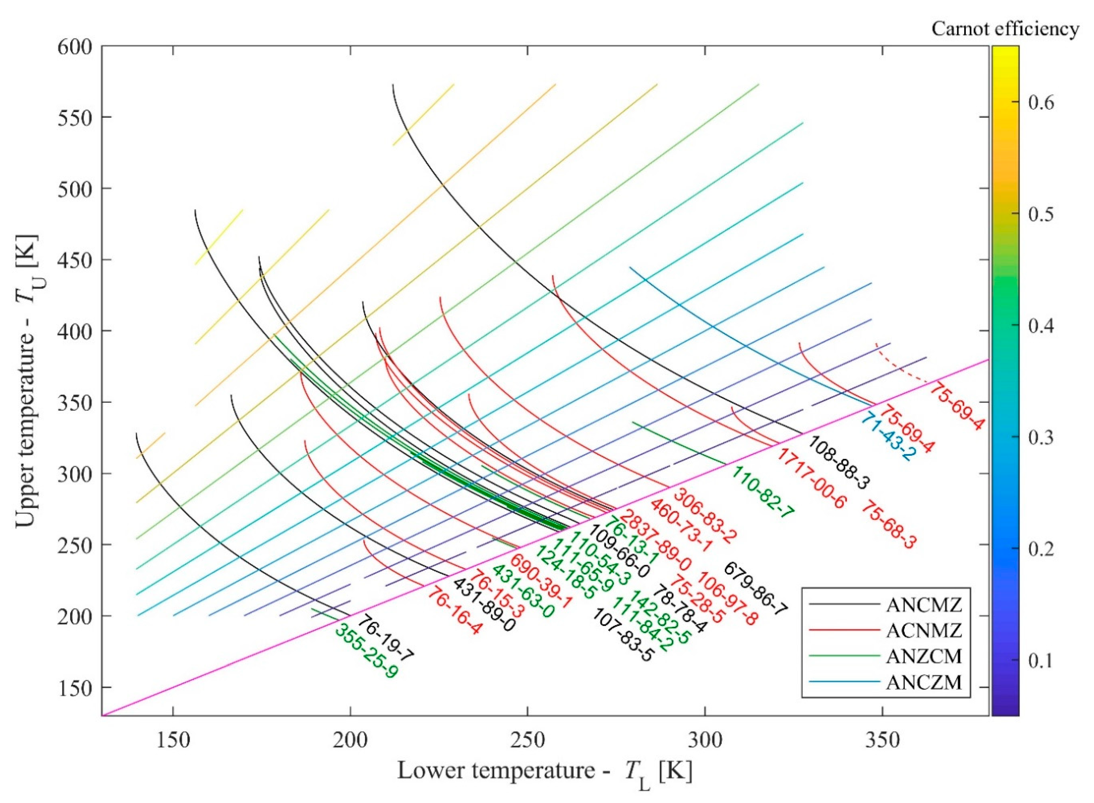
Using 28 materials with reverse S-shaped vapour branch and with T-s diagrams available in the NIST databases (NIST Chemistry WebBook [15] and from RefProp 9.1 [16]), one can construct a map for all potential routes; this map is shown in Figure 2. The lower end for all lines are on one curve, defined by the N-points; for the shortest possible expansion route T_U = T_N + δ and T_L = T_N + δ, where T_N refers to the temperature corresponding to point N and δ is an infinitesimally small temperature difference with δ → 0. For this reason, the lower limit should be located on a straight line with slope = 1, where T_U = T_N = T_L. Marking this lower limit, one can avoid unrealistic T_L > T_U cases.

Materials are identified by their chemical identifier (CAS number). When lines are congested, labels are following the order of lines in zig-zag. Materials corresponding to various classes are plotted in various colors; black for ANCMZ, red for ACNMZ, green for ANZCM and blue for ANCZM; as it was already mentioned, materials with ACNZM sequences have not been found up to now. For additional information, Carnot-efficiencies for a given upper and lower temperature pair are given by color-coded lines. The list of materials with their CAS-number, name, refrigerant code (if any) and classification can be found in

Table 1. List of materials used in the study. The list follows the order of Figure 2 starting at decafluorobutane, marked as 355-25-9 to trichlorofluoromethane (also referred as R11), marked as 75-69-4.

CAS-Number	Name	R-Number	Class
355-25-9	decafluorobutane	-	ANZCM
76-19-7	perfluoropropane	R218	ANCMZ
76-16-4	freon 116	R116	ACNMZ
431-89-0	propane, 1,1,1,2,3,3,3-heptafluoro-	R227ea	ANCMZ
76-15-3	freon 115	R115	ACNMZ
431-63-0	1,1,1,2,3,3-hexafluoropropane	R236ea	ANZCM
690-39-1	1,1,1,3,3,3-hexafluoropropane	R236fa	ACNMZ
107-83-5	2-methylpentane (isohexane)	-	ANCMZ
124-18-5	decane	-	ANZCM
111-84-2	nonane	-	ANZCM
111-65-9	octane	-	ANZCM
142-82-5	heptane	-	ANZCM
110-54-3	hexane	-	ANZCM
78-78-4	2-methylbutane (isopentane)	R601a	ANCMZ
109-66-0	pentane	R601	ANCMZ
76-13-1	freon 113	R113	ANZCM
75-28-5	2-methylpropane (isobutane)	R600a	ACNMZ
106-97-8	butane	R600	ACNMZ
2837-89-0	freon 124	R124	ACNMZ
679-86-7	1,1,2,2,3-pentafluoropropane	R245ca	ANCMZ
460-73-1	1,1,1,3,3-pentafluoropropane	R245fa	ACNMZ
306-83-2	freon 123	R123	ACNMZ
110-82-7	cyclohexane	-	ANZCM
1717-00-6	1,1-dichloro-1-fluoroethane	R141b	ACNMZ
75-68-3	ethane, 1-chloro-1,1-difluoro-	R142b	ACNMZ
108-88-3	toluene	-	ANCMZ
71-43-2	benzene	-	ANCZM
75-69-4	trichlorofluoromethane	R11	ACNMZ

.

Since T-s data are available in various sources, NIST-based data (NIST Chemistry Webbook [15] and RefProp 9.1 [16]) has been cross-checked. Visible difference was found only in one occasion (CAS 75-69-4, trichloromonofluoromethane, also called R11 or Freon 11); the alternative curve (data are taken from FluidProp [18], using TPSI model, based on the work of Reynolds [19])) is also plotted by the dashed red line.

Carnot-efficiencies are also shown in Figure 2. These values are characteristic for the given heat source—heat sink pairs. Being the corresponding T_U and T_L values are external constraints, Carnot-efficiencies cannot be improved. They are shown here (and later in similar figures) to give some indication about the theoretical efficiency maximum as a benchmark.

In the next sections, comparison of T_L-T_U diagram of real materials (where “real” refers to data taken from well-established reference equations) with T_L-T_U diagram of model fluids (van der Waals fluid) is given; this way one might be able to single out erroneous data. Then, the method to find the working fluid which can be used with the simplest layout for a given heat source—heat sink pair by using the T_L-T_U diagram of real fluids is presented.

3. Comparison of Reduced T_L-T_U Diagrams

The behaviour of fluids can be described with various equations of states (EoS); usually simple, easily solvable equations are giving less accurate descriptions than more complex, sometimes even non-analytical ones. Luckily, the results given by some of these simple EoS are qualitatively acceptable, therefore they can be applied for comparison purposes. Concerning T-s diagrams, two model fluids has been studied earlier, using van der Waals [8] and Redlich-Kwong [10] EoS. One of the advantages of using simple EoS is to reduce the possibility to obtain mathematical artefacts caused by some more accurate, but mathematically more complex EoS (see for example the misplaced second critical point given by the very accurate water EoS, the IAPWS [20]). Therefore, the van der Waals EoS with temperature independent molecular degree of freedom has been used to obtain the “theoretical” T_L-T_U diagram. The result can be seen in Figure 3. Model materials corresponding to various classes are plotted in various colors, also used for Figure 2. Concerning the qualitative agreement mentioned above, it is interesting to see, that the class missing in case of real materials (ACNZM) is also missing here.

One can realize, that the curves are located within a triangle. The lower boundary is defined by the coordinate of the N points, similarly to Figure 2. Concerning the upper boundary (magenta line), these are the T_L and T_U values for the “longest” expansion lines for classes ACNMZ (red) and ANCMZ (black), namely the points defined by temperatures corresponding to ${\mathrm{M}}_{\mathrm{s}}^{\mathrm{d}}$ (as T_L) and M (as T_U). The exact shape of this curve is not clarified, but it seems to be close to linear. Concerning the third side of the triangle, it is an artificial limit (therefore it is not marked by a line), caused by the fact that all T-s diagrams of van der Waals fluids have been calculated in the same reduced temperature range (from T_r = 0.3 to T_r = 1), where the reduced temperature is the actual temperature divided by the critical one. Although this limit seems to be artificial, it reflects correctly, that the “liquid range” of materials located between the triple point and the critical point is usually in the 0.4–1 reduced temperature range for most of the materials [21]. The temperature of these “lowermost points of the liquid state” are identical with the temperatures of point Z (and also with point A), therefore the “longest” expansion lines for classes ANCZM (blue) and ANZCM (green), are terminated on a line formed by the upper and lower expansion end-points, defined by temperatures corresponding to Z (as T_L) and ${\mathrm{Z}}_{\mathrm{s}}^{\mathrm{u}}$ (as T_U).

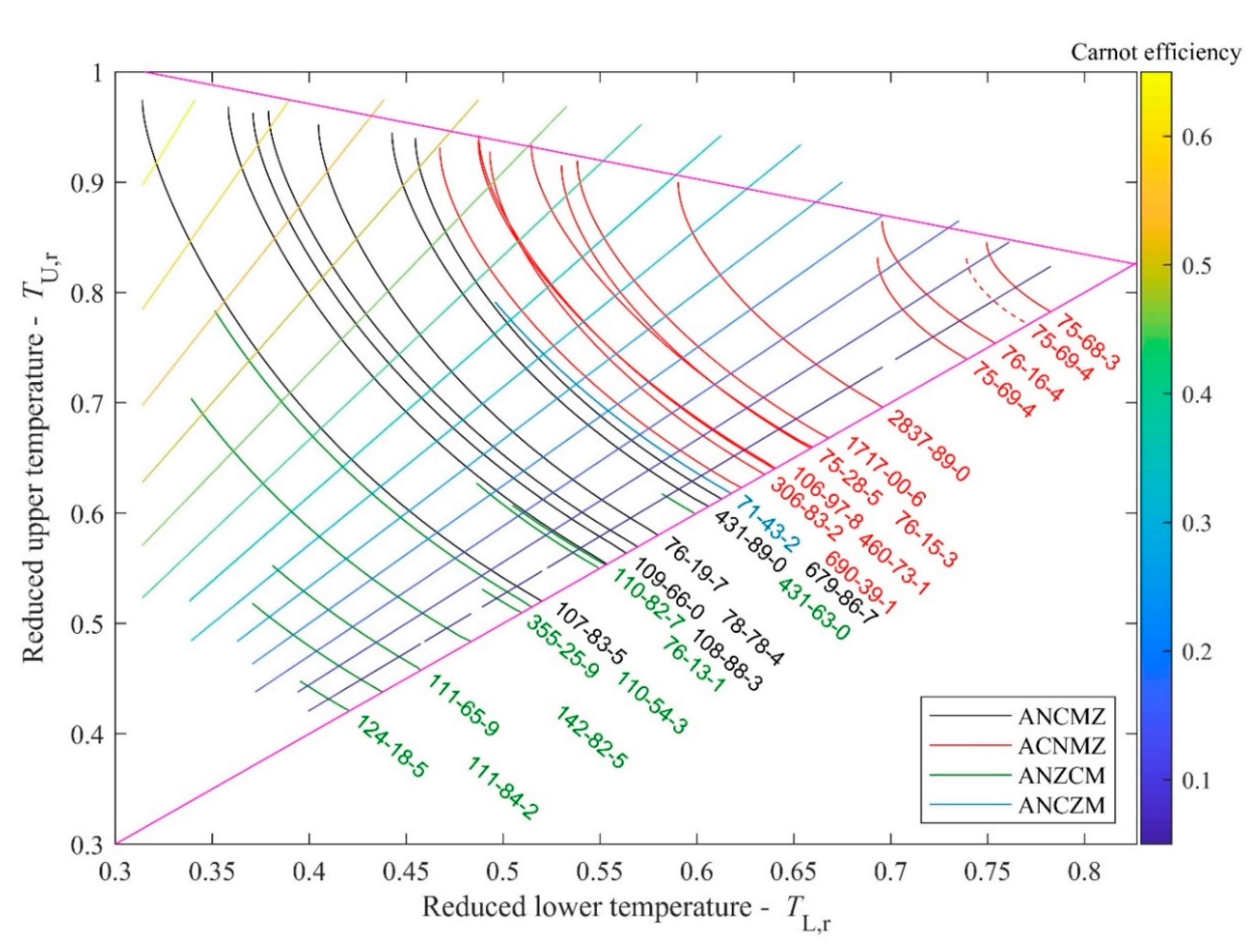
For comparison, the reduced T_L-T_U diagram for the real materials (shown in Figure 2) can be seen in Figure 4. The real curves are also located in a triangular region. The lower border is as sharp as before, because it is the slope = 1 line, defined by the identical T_U and T_L temperatures of points N. One can also see an upper boundary defined by temperatures corresponding to ${\mathrm{M}}_{\mathrm{s}}^{\mathrm{d}}$ (as T_L) and M (as T_U). While for the model fluid, this upper boundary for ANCMZ (black) and ACNMZ (red) classes is quite sharp, one can see that it is less defined here. Concerning the third side of the region, it can be noted that the expansion line for most of the materials in the ANZCM class (green) terminate in the reduced T_L = 0.35–0.4 region (as it is “expected” from the thumb-rule between melting and critical temperatures, see for example [21]), but the remaining part of the ANZCM-class materials as well as the only ANCZM-one terminate at higher reduced T_U temperatures, showing much narrower liquid region between freezing and critical point.

Concerning trichlorofluoromethane (CAS 75-69-4), which has a different representation using NIST-based data or Stanford (TPSI)-based data, it seems that both curves are too short (they terminate much below the upper boundary), but the TPSI-data seems to be better. For other materials, no visible differences have been found. From the data obtained by van der Waals EoS, one can see the existence of an upper envelope of the curves. Therefore, one can expect that for real materials, the curves will also be confined between an upper and a lower borderline. It means that for example shorter expansion lines of ACNMZ class fluids should be located on higher T_L,r temperatures, than longer expansion lines. Hence, the short solid line representing trichlorofluoromethane (R11, 75-69-4) is probably misplaced and it should be located above the expansion line of freon-116 (76-16-4) and not below it. Consequently, the dashed red lines based on TPSI-data seems to be better than the one, based on NIST data.

On one hand, by using reduced temperature data, the structure of T_L-T_U diagram are much clearer now; also it can help to single out erroneous data. On the other hand, for the selection of the optimal working fluid for a given heat source—heat sink, the use of the original T_L-T_U diagram is necessary, as it will be shown in the next section.

4. Selection Process of the Thermodynamically Optimal Working Fluid

Concerning an existing heat reservoir, one has to use a fixed maximal or upper temperature (T_U) for the cycle, given by the heat source temperature (T_source) and the pinch temperature (ΔT, a characteristic value for the heat exchanger) as:

$$T_{\mathrm{U}} = T_{\mathrm{source}}-\mathsf{\Delta }T$$

(1)

In a similar manner, the lowest temperature of the cycle (T_L) can be defined by the temperature of the environment used for cooling (T_environment) and a lower pinch temperature (not necessarily equal with the other one) as:

$$T_{\mathrm{L}} = T_{\mathrm{environment}} + \mathsf{\Delta }T$$

(2)

This (T_U; T_L) pair can be used as a characteristic point in Figure 2 to represent a given heat source and sink with other technical details such as quality of heat exchangers; since for reduced quantities, the critical temperature of the working fluid is also necessary, therefore on reduced diagrams (like Figure 3), the reduced (T_U; T_L) points alone cannot be used to characterize the heat source and heat sink of the system.

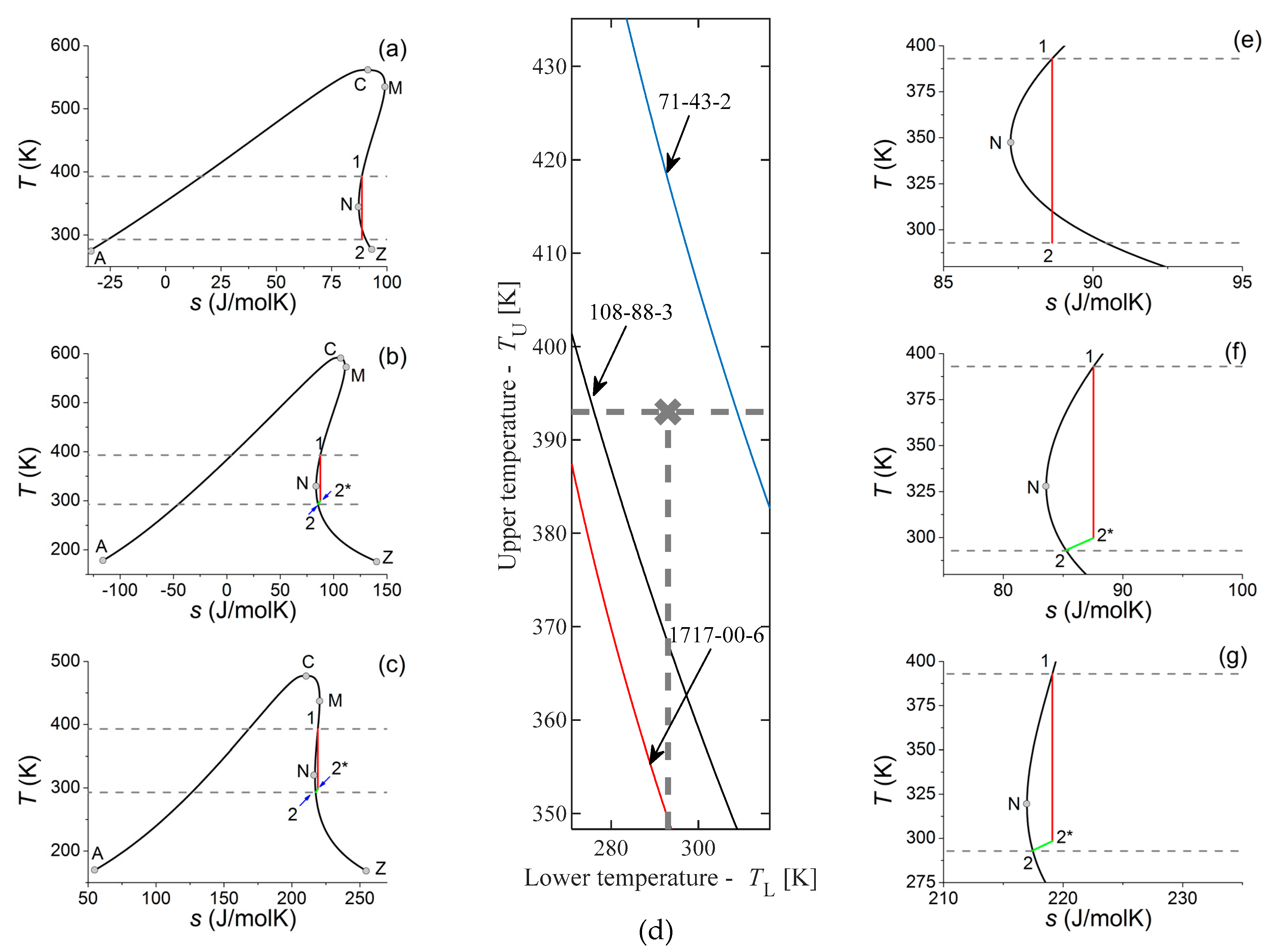
In Figure 5d, the grey cross represents a hypothetical heat source and sink characterized by T_U = 293 K = 19.85 °C and T_L = 393 K = 119.85 °C. This can be for example a geothermal heat reservoir with a natural cold water source (a small river) or cold internal air (winter) used for cooling. This situation is very similar to the first (and presently only) ORC-based Hungarian geothermal power plant (see the ORC Word Map [22]).

In Figure 5d, only part of the data presented in Figure 2 can be seen, centered on the (293K, 393 K) point. This point is located between two lines representing two working fluids, namely benzene (CAS 71−43−2) and toluene (CAS 108−88−3); one more material can be seen here, namely the 1,1−dichloro−1−fluoroethane (CAS 1717-00-6, also referred as R141b). Since none of these lines run through the 293−392 K point, the closest ones (benzene and toluene) should be considered as nearest to ideal. For the sake of completeness, the potential use of the third one (R141b) is also discussed. The upper and lower temperatures determine the extent of expansion, as it can be seen in Figure 5a,e (benzene), Figure 5b,f (toluene) and Figure 5c,g (R141b).

For further discussion, one can define the so-called quality (q), also referred as dryness or dryness fraction of pure fluids, representing the ratio of vapour within the two-phase region and defined as:

$$q = \frac{n^v}{n^l + n^v}$$

(3)

where n^v and n^l are the mole- (or alternatively, the mass-) fraction of the fluid in the vapour or liquid phase, respectively. This quality can change between one (saturated vapour) and zero (saturated liquid); outside of the two-phase region, it is usually not defined or defined as one (vapour states) or zero (liquid states). This ratio can be also calculated by using the specific entropy values for the given mixed state and comparing it with the entropy values of the saturated liquid and vapour states at the same temperature [23].

In the case of benzene (Figure 5a,e), one can see that the expansion route started at saturated vapour state at 393 K and terminated at 293 K, runs in superheated dry vapour region for a while, but the final part of the expansion (starting from 309.96 K down to 293 K, i.e., in an almost 17 K temperature range) runs into the two-phase, wet region. The maximal q value (corresponding to the final state of the expansion) is 0.9848, equal to 1.52% (in mass) of droplet. Droplets may cause erosion problems, moreover they might decrease the net efficiency due to moisture loss, although this 1.52% is not very high compared to the 8–12% which is usually considered tolerable [24]. For benzene, the ideal case—i.e., expansion from one saturated vapour state to another saturated vapour state—would be the termination of expansion at T_L = 309.96 K, given by the cross section of the blue line (representing benzene) and grey dashed line (representing T_U = 393 K). Stopping at this higher temperature would cause smaller efficiency, therefore the problem of droplet erosion should be weighed against the problem of potential efficiency loss, before deciding the use or omission of benzene. It also means that benzene would be the ideal working fluid (concerning only the expansion route and neglecting other selection criteria) for a heat source and sink characterized by (T_U, T_L) = (393 K, 309.96 K) temperatures.

In case of toluene (Figure 5b,f) if the expansion route starts at saturated vapour state at 393 K and terminates at 293 K, than even the final part of the expansion runs in superheated dry vapour states. Therefore one would not face challenges regarding droplet formation. Unfortunately, another problem emerges, namely the problem of cooling down the expanded dry vapour in an isobaric way before reaching saturated vapour state at T_L = 293 K. Therefore, isentropic expansion (solid red line) has to be stopped at a higher temperature (point 2*, T = 299.7 K) and the rest of the process (2*→2) has to proceed on an isobaric cooling route (green line). In this way, a small, almost triangle shaped part in the T-s diagram (formed by the grey line, the green line and by the extension of the red one) will be excluded from the cycle, decreasing the thermal efficiency. As an additional problem, this unused (lost) heat can increase the heat-load of the environment. Addition of a recuperative heat exchanger to the system can solve—or at least minimize—these problems, since part of this heat can be used to pre-heat the compressed liquid. This solution is appropriate only if the temperature difference between point 2* and 2 is large enough. In case of toluene with 393–293 K expansion, this gap is around ΔT = 7 K, which can be used only in a very limited manner for this purpose. With a larger gap, this heat can be utilized better, however the thermal efficiency is still smaller, therefore the goal remains to reach a perfect “saturated steam to saturated steam” expansion route, with zero gap. Similarly to the case of benzene, one can define an ideal T_L, where expansion from T_U would be terminated at the saturated vapour state; for toluene it would be 276.06 K. It means, that toluene would be the ideal working fluid (concerning expansion route) for a heat source and sink characterized by (T_U, T_L) = (393 K, 276.06 K) temperatures.

In case of R141b (Figure 5c,g) the situation is very similar to the one observed for toluene. The expansion—even in the final stage—runs in superheated dry vapour region, so droplet-related problems do not exist. Similarly to toluene, isentropic expansion has to be stopped at a temperature above 293 K, namely at the one marked as 2* (here it means 298.5 K) and the rest of the process (2*→2) has to proceed on an isobaric cooling route, losing some part of thermal efficiency and increasing the heat-load of the environment. Here, the temperature gap between points 2* and 2 is 5.5 K, which is probably too small to use recuperator. Similarly to the case of benzene and toluene, one can define an ideal T_L, where expansion from T_U would be terminated at the saturated vapour state; for R141b it would be 268.2 K, almost 8 K lower than for toluene. It means, that R141b would be the ideal working fluid (concerning expansion route) for a heat source and sink characterized by (T_U, T_L) = (393 K, 268.2 K) temperatures. One should realize, that for materials on the dry side, but “farther” from the point characterizing the heat source and heat sink (here, toluene is closer, R141b is farther), the expansion has to be stopped farther on temperature scale from the saturated liquid state, but this temperature distance does not correlate with the temperature difference between points 2* and 2. For R141b, the “belly” of the inverse S-shape is smaller than for toluene, therefore the temperature gap between points 2* and 2 is smaller for R141b than for toluene, despite the fact that R141b is farther from the characteristic point. Therefore, R141b might be better for this given heat source and heat sink system, than for toluene, i.e., not only the immediate, but second (or even further) neighbours should be checked in the selection process.

Table 2. Total (η_br) and net (η_net) cycle efficiencies—calculated in CycleTempo 5.0 environment using fluid data from RefProp 9.0—of ORCs using working fluids presented in Figure 5 and Figure 6. For net efficiencies, self-consumption of pumps were deducted. Temperatures are shown here not only in K, but also in Celsius, according to engineering practice. Values for qualities at the end of expansion are also shown (q). Details of calculations can be seen in Supplementary materials.

TL	19.85 °C	19.85 °C	19.85 °C	−44.65 °C	−44.65 °C	−44.65 °C
	293 K	293 K	293 K	228.5 K	228.5 K	228.5 K
TU	119.85 °C	119.85 °C	119.85 °C	29.85 °C	29.85 °C	29.85 °C
	393 K	393 K	393 K	303 K	303 K	303 K
material	benzene	toluene	R141b	pentane	isopentane	hexane
CAS	71-43-2	108-88-3	1717-00-6	109-66-0	78-78-4	110-54-3
br	21.72%	21.65%	21.05%	21.23%	21.21%	21.28%
net	21.66%	21.63%	20.79%	21.21%	21.18%	21.27%
Ppump	−2.75 kW	−1.26 kW	−12.55 kW	−1.04 kW	−1.46 kW	−0.31 kW
Pturb	1000 kW	1000 kW	1000 kW	1000 kW	1000 kW	1000 kW
q	98.48%	100.00%	100.00%	99.52%	100.00%	100.00%

summarizes the data which compares the efficiencies of cycles using various materials. Details of the calculations are given in the Supplementary Materials. For all materials, the total efficiencies are in the 21.05–21.72%, and the net efficiencies are in the 20.79–21.66% range. With such small differences—especially for benzene and toluene—the difference of operational (including maintenance) and investment costs by using the simplest layout can be a decisive factor by choosing working fluids. In this case—since the ideal fluid has not been found—the cost related to the presence of droplets has to be compared with the costs related to the installation and operation of the recuperator. Since the use of recuperator are not justified here, toluene seems to be the better choice in the given temperature range; its net efficiency matches the efficiency of benzene but droplets would not be present to cause erosion-related problems. Obviously, using other parameters for the optimization process, other fluids might perform better.

Unfortunately, none of the expansion routes of known working fluids run through the (393 K, 293 K) point, therefore one can choose only something “close enough”. Another alternative would be—especially when there are two “close enough” working fluids with chemically similar structure, like toluene and benzene—the application of a mixture. Due to the chemical similarity, the mixture would be probably an almost ideal, zeotropic mixture, which can be used more easily as working fluid in ORC applications than azeotropic ones [8,25,26].

Concerning lower temperatures, one can see regions on the T_U-T_L diagram densely packed with expansion routes. Recently, there are more and more applications for liquid methane (LNG). LNG can be transported to LNG-terminals by ships, and there they must be re-gasified before injected into the regular gas network, giving the possibility to utilize the so-called “cold energy” [27,28]. Concerning the fact, that the temperature of liquid methane can be as low as 111 K (−162 °C), the external heat used for re-gasification can be even the environmental heat (air, water), around or below 300 K. Obviously, going down to 111 K in an ORC would cause some serious problems concerning materials used for the construction, but using the methane as heat sink and cooling the chosen working fluid down only to a moderate level, one can define an acceptable expansion range for example between T_U = 303 K and T_L = 228.5 K. Here, the lower temperature is only an arbitrarily chosen, but plausible value to demonstrate the selection process; for any other temperature, the selection process would be the same, only the optimal working fluid would be different. In Figure 6d, one can see part of Figure 2 centered around this point. It is clearly visible, that one line runs almost exactly through this point, namely the line representing 2-methylbutane (isopentane, CAS 78-78-4) and it is slightly off from the lines representing two linear alkanes, hexane (CAS 110-54-3) and pentane (CAS 109-66-0). Expansion lines for these three working fluids are shown in Figure 6a,e (pentane), Figure 6b,f (2-methylbutane) and Figure 6c,g (hexane).

First, the potential use of pentane is discussed. In this case, the end of the expansion runs into the two-phase (wet) region (see Figure 6a,e), but in a much smaller extent, than it was shown for benzene. Here, the expansion line enters the two-phase region around 232.8 K, only 4.3 K above the end of the expansion process. The quality of wet steam will be 0.9952, corresponding to 0.48% wetness, half of the value reported in the previous case. In the case of benzene, the wetness was already in the tolerable level; it is even more valid for this case.

By using 2-methylbutane, the expansion between T_U = 303 K and T_L = 228.5 K starts and terminates in saturated vapour states, avoiding all problem related to wet or superheated dry vapour. This is shown in Figure 6b,f. Concerning the expansion route, this is the perfect working fluid for a heat source and heat sink pair, represented by T_U = 303 K and T_L = 228.5 K.

Finally, the use of hexane is discussed. In this case, the expansion should be terminated within the dry vapour region and the working fluid has to be cooled down to T_L by isobaric cooling. Here, the isobaric part is so small, that it can be hardly seen even on the magnified figure (Figure 6c,g); the expansion has to stop at 228.97 K, instead of 228.5 K, only 0.47 K above the T_L. This small gap cannot be utilized for pre-heating the pressurized liquid, but the heat loss caused by this part is negligible.

For these materials, total cycle efficiencies move in the very narrow 21.21–21.28% range, while their net counterparts are in the 21.18–21.27% range. With such small differences, the difference of operational and investment costs by using the most simple layout can be a decisive factor by choosing working fluids; in this case, the most simple layout can be realized by using 2-methylbutane, without the loss of efficiency. Obviously, other parameters of optimization might give a different result, but for our criteria, this is the best-performing working fluid for the given temperature range. It should be noted here, that being the three materials chemically similar, some of their chemistry-related properties (like ODP, GWP, toxicity, flammability) are quite similar, and therefore the indicators related to these properties are also similar.

In the case of T_U = 303 K and T_L = 228.5 K, one can pinpoint the ideal working fluid, where expansion would run from one saturated vapour state to another saturated vapour state, all along a dry vapour route. At the end of the expansion, the final state would be a saturated vapour state, therefore the problems caused by wet or superheated dry vapour (discussed above) do not exist! This ideal working fluid would be the 2-methylpentane. Due to the fact that expansion routes for several materials run in the immediate vicinity of this (T_U, T_L) = (228.5 K, 303 K) point, one can even find a second-, third-, fourth-best; this is especially important, when the working fluid chosen as “best” for our criterion performs worse, when another important optimization criterion is considered. Because these routes are close to our working point, using one of them—instead of the ideal one—would cause only minor problems, acceptable for the given application. For this temperature range, the ones next to the best would be pentane and hexane; using them the problems caused by the presence of droplets or superheated dry vapour are almost negligible, therefore their application (and probably the application of several other working fluids with expansion range lines running close to the (T_U, T_L) = (228.5 K, 303 K)) would be acceptable. In this way, one could use other criteria (environmental safety, chemical compatibility, price, availability, etc.) together with some optimization method (see for example [29,30,31]) to choose the proper working fluid, still acceptable thermodynamically, but not necessarily the best one according to this criterion.

5. Conclusions

A novel method has been proposed to choose the best working fluid—from the point of view of expansion route—for a given heat source and heat sink (characterized by a maximum and minimum temperature). The method is based on the novel classification of working fluids using the sequences of their characteristic points on temperature-entropy space [11]. Using this simple method, a possible expansion route can be defined between an upper and lower temperature values; these temperatures are characterizing the given heat source, heat sink and the set of heat exchangers. In this way, one can select a working fluid (from a database, see [14]), where an ideal adiabatic (isentropic) expansion process between a given upper and lower temperature is possible in a way, that the initial and final states are both saturated vapour states and the ideal (isentropic) expansion line runs in the superheated dry vapour region all along the expansion. In this way, it is possible to avoid problems related to the presence of droplets or superheated dry steam in the final expansion state, just before the condensation. Therefore, one can use the most simple ORC layout, using only a pump, two heat exchangers (evaporator, condenser) and an expander, avoiding the use of superheater (or droplet separator) and recuperator; since the fluid is always in dry condition during expansion, droplet erosion can also be avoided.

Study of potential expansion routes in van der Waals model fluids and comparison of the results with the one obtained with real working fluids can help us to single out erroneous data of working fluids presented in various databases.

Presently we have a database of nearly 30 pure fluids with T-s data taken from the NIST Chemistry WebBook [15] and from RefProp 9.1 [16]. Most of these fluids were termed formerly as “dry”, while in the novel classification they are in various isentropic sub-classes, namely in ANCMZ, ACNMZ, ANZCM and ANCZM. Due to the fact, that the characteristic point responsible for the existence of these expansion routes (point N) is usually located at low temperature for most of the materials of our database, presently this method with the existing, highly accurate database can mostly be used to choose the working fluids thermodynamically most suitable for cryogenic cycles (applied for example for heat recovery during LNG-regasification, see for example [27,28], although some of the materials can be used in higher temperatures (covering part of the temperature range for geothermal and waste heat utilization).

Extension of the method (including internal efficiencies below 1 for the expander as well as acceptable wetness for the final vapour state) and expansion of the database with more material are in progress. After a proper extension of the database, this method will be available to choose ideal working fluids for other temperatures (like the ones characteristic for various geothermal or waste heat applications).