In this section, the convergence of the CFD model is first investigated. Then, the CFD model is validated by comparing the predicted hydrodynamic responses with both experimental and BEM results. Finally, the hydrodynamic nonlinearity identified by the CFD model and the hydrodynamic force distribution along the longitudinal direction of the Duck are studied.
5.1. Convergence Study of the CFD Model
Before the CFD model is used to perform hydrodynamic simulations of the solo Duck WEC, it should be both mesh and time step resolution independent.
Figure 6a,b show the measured free surface elevation
h at the Duck position with the Duck be removed from the NWT, and hydrodynamic responses of the Duck at wave period
T = 1.6 s and wave height
H = 0.075 m. Here,
τ is the non-dimensional flow time defined by the flow time
t divided by the wave period. In both subfigures, the curves behave in an approximately sinusoidal way. The variation of the measured wave height only depends on horizontal and vertical, i.e., the
x and
z direction, mesh resolution. Therefore, convergence of the mesh resolution in horizontal and vertical directions is investigated with measured wave height as the dependent variable. On this basis, when the Duck is embedded into the NWT, the variation of the pitch angular displacement amplitude
θ5 only depends on the longitudinal, i.e., the
y direction, mesh resolution and the time step resolution. Hence convergence of the longitudinal mesh resolution and the time step resolution will be studied with pitch angular displacement amplitude as the dependent variable. Since small vibrations of both
H and
θ5 are observed due to wave reflection, the two dependent variables are averaged over three wave periods for comparison. In
Figure 6b, the surge and heave hydrodynamic forces represent the forces applied by the water in the
x and
z direction, respectively.
Figure 7 shows the convergence study results at
T = 1.6 s and
H = 0.075 m.
Figure 7a shows the measured wave height as a function of the cell number per wavelength and per wave height. The wave height tends to be stable when the cell number per wavelength and per wave height exceeds 30 and 10, respectively.
Figure 7b shows the pitch angular displacement amplitude as a function of the cell number in the longitudinal direction and per wave period. Also, it reveals that when the cell number in the longitudinal direction and per wave period exceeds 32 and 360, respectively, the angular displacement amplitude tends to converge. Therefore, for a tradeoff betweenthe computational costand the accuracy, for later simulations in this paper, the mesh resolution and time step are set according to the critical cell number stated above.
5.2. Comparison in Different Wave Heights
Table 2 shows the test cases for the comparison in different wave heights.
Figure 8 shows the comparison of the pitch angular displacement amplitude as a function of wave height among CFD, BEM and experimental results at
T = 1.6 s. In
Table 2, the difference of the wave height between the CFD and experimental model is due to the measured wave height at the position of the Duck being different from the set value at the wave maker. For example, if the set value of the wave height at the wave maker is 1.0 cm, the measured value of the wave height at the position of the Duck may be smaller than 1.0 cm. The reason behind this phenomenon is that the wave energy is dissipated during the propagation process. Since the dissipation rate of the wave energy may be different between the CFD and experimental model, the measured wave height at the position of the Duck may also be different, e.g., 0.9 cm for the CFD model and 0.8 cm for the experimental model. Therefore, the expectation of realizing an identical value of the wave height at the position of the Duck for both the CFD and experimental models cannot be easily achieved, but needs time-consuming tuning of the set value of the wave height at the wave maker for both models. Besides, since the wave height is served as the independent variable in
Figure 8, whether or not the wave height in the CFD and experimental model is the same does not influence the variation tendency of the dependent variable. Therefore, the wave height between the CFD and experimental model needs not to be the same. The maximum of the wave height in the CFD model is larger than that of the experimental model due to capsizing of the Duck. Due to friction, the motion response of the Duck in the experimental model is slightly smaller than that in the CFD model. Therefore, the Duck in the experimental model is harder to capsize. Meanwhile, the maximum wave height in both models is the minimum wave height that induces the Duck to capsize. Therefore, the maximum of the wave height in the experimental model is larger than the CFD model.
For all three models, the pitch angular displacement amplitude grows with wave height. CFD results agree well with BEM results at small wave heights, and presents almost linear relationship with wave height. However, at large wave heightswhen
H ≥ 0.12 m, difference emerges since the CFD curve shows a slower growing trend while the BEM one shows the same slope as at small wave heights. Actually, this can be explained by the hydrodynamic nonlinearityinduced at large wave heights. In [
32], it is found that BEM models without the nonlinear term of drag force over-estimate the response of the WEC when compared to CFD models. For cases with high wave heights, the influence of the drag force will be more prominent since the magnitude of the drag force increases with the square of velocity. Compared to experimental results, the CFD curve shows the same tendency as the experimental one, but predicts an overall larger value, especially at small wave heights. A possible explanation for these phenomena is the friction loss in the mechanical transmission system. Actually, friction is very complex and its formation mechanism has still not been clearly revealed yet. Friction also varies nonlinearly with a lot of parameters, such as the velocity. For a Duck WEC, since the Duck oscillates periodically, the velocity of the Duck varies all the time, thus a fixed value of the friction cannot be obtained. Han et al. [
33] tried to take friction into consideration by tuning the value of the friction inside the numerical model until the response of the numerical model equals that measured in the experimental model. However, for the comparison between the numerical and the experimental model in this paper, the friction cannot be determined ahead. Anyway, although there are differences between the numerical and experimental model, the difference is not significant overall, and experimental results can still quantitatively validate the numerical models to some extent.
Figure 9 shows the comparison of the hydrodynamic force amplitude as a function of wave height at
T = 1.6 s. Both surge and heave forces grow almost linearly with wave height. Similar to the variation tendency of pitch angular displacement amplitude with wave height, CFD results agree well BEM results at small wave heights, while diverges from BEM results at large wave heights with the heave force as an exception. Compared to experimental results, CFD results show only small difference in the whole wave height range. The main reason is that the friction in the mechanical transmission system does not influence the pressure distribution around the Duck. Therefore, the hydrodynamic forces are not influenced by the friction.
5.3. Comparison in Different Wave Periods
In this section, the comparison is performed in a range of wave periods, from 0.6 s to 2.0 s.
Table 3 shows the test cases for the comparison in different wave periods.
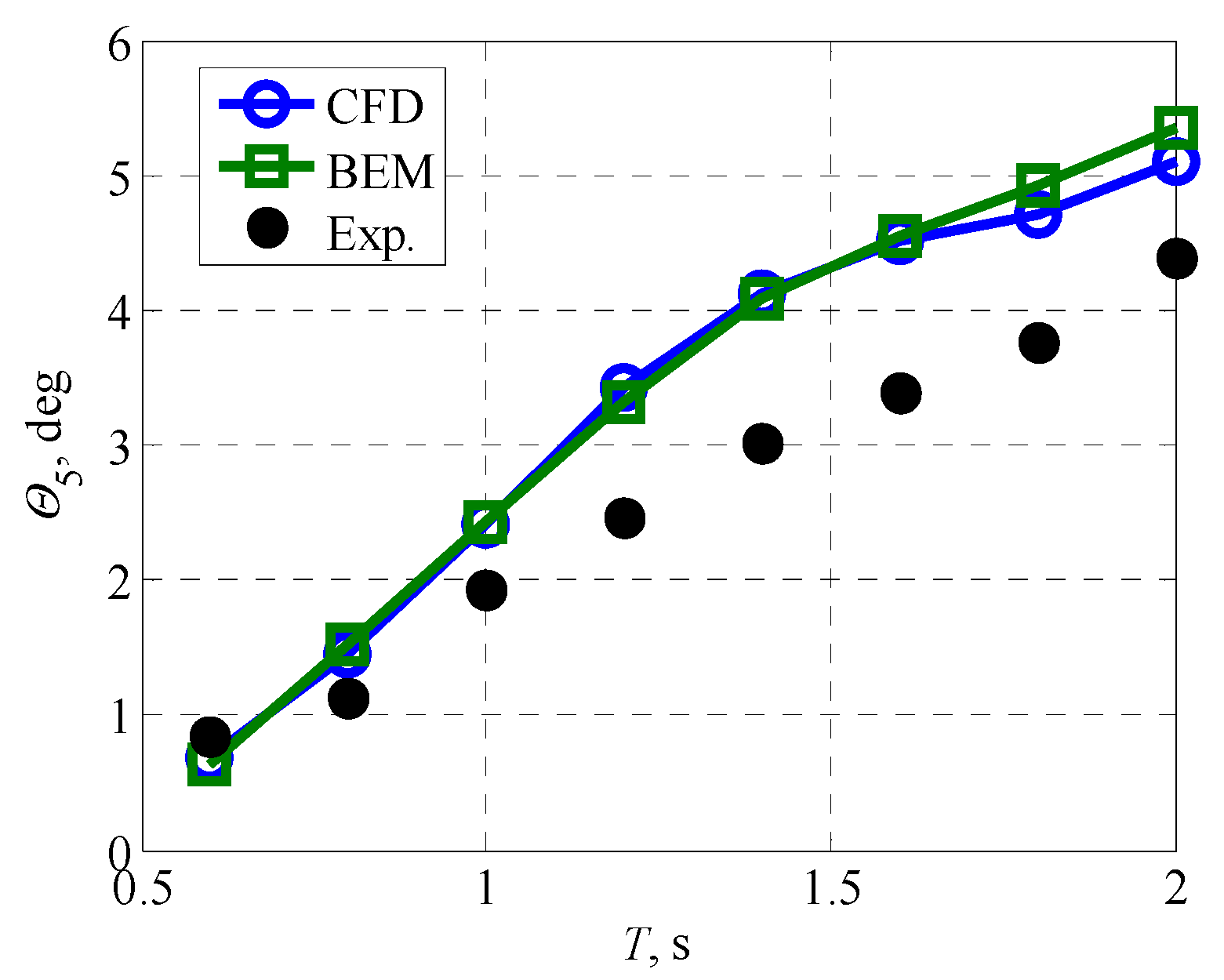
Figure 10 shows the comparison of pitch angular displacement amplitude as a function of wave period among CFD, BEM and experimental results at
H = 0.075 m. For all three models, the angular displacement amplitude grows with wave period. CFD results agree well and almost coincides with BEM results when
T ≤ 1.4 s. When
T > 1.4 s, CFD results are slightly smaller than BEM results. The difference is expected to be resulted from the viscosity that damps the response of the Duck in the CFD model. The angular displacement amplitude predicted by the CFD model is larger than experimental results a most wave periods except at
T = 0.6 s and the discrepancy grows with wave period.
Figure 11 shows the comparison of the hydrodynamic force amplitude as a function of wave period at
H = 0.075 m. In
Figure 11a, the surge force amplitude peaks at
T = 1.4 s and decreases gradually on either side for all three models. The surge force amplitude of CFD resultsshow little difference from experimental resultswithin the wave period range from 0.8 s to 1.4 s, while is smaller than experimental results when
T ≤ 0.8 s, and larger than them when
T ≥ 1.4 s. Compared to BEM results, the force predicted by the CFD model is slightly larger in the whole wave period region. In
Figure 11b, the heave force amplitude grows with wave period for all three models. In fact, these amplitudes equal the surge and heave excitation force since the WEC is static in both degrees of freedom. The shape of the curves is characterized by either a bell-like shape with the peak value appears at the wave period of 1.4 s, or by a nearly monotonically varying trend. The data that forms the shape can be approximately obtained by solving the Laplace equation, with the boundary condition defined by the geometry of the WEC. Therefore, the shape of the curves, no matter it is the bell-like form for the surge mode or the nearly straight form for the heave mode is influenced mostly by the geometry of the WEC. The difference between CFD and experimental results is smaller than that between BEM and experimental results. One possible reason for the discrepancy between CFD and experimental results may be the installation error of the mechanical equipments, which may cause the measured surge and heave excitation forces be coupled with the excitation force of other degrees of freedom. The complex coupling effect may cause the resultant measured excitation force from the experiment be larger than that of the numerical models. From above comparison results, it is revealed that the CFD model can better predict the hydrodynamic response of the Duck than the BEM model for this experimental setup.
5.4. Influence of Wave Steepness
From the comparison performed in
Section 5.2 and
Section 5.3, we find that the difference of the predicted hydrodynamic responses between the CFD and BEM models appears at different wave heights and wave periods.In order to quantitatively describe the difference of predicted results between the CFD and BEM model, the concept of relative difference is introduced as:
where
φCFD denotes results from the CFD model and
φBEM for the BEM model. Relative difference is defined to measure to what extent the two results differ from each other.
Figure 12 shows the relative difference of pitch angular displacement amplitude as a function ofwave height and wave period. It can be seen that the relative difference between the CFD and BEM model generally increases with wave height, but decreases with wave period.
Since the BEM model is linearised from the CFD model, we can attribute the above difference to the hydrodynamic nonlinear factors that are taken into consideration in the CFD model, including the nonlinearity of the wave, i.e., the nonlinear waveform, and the nonlinearity of the Duck motion, i.e., the vortex generation process. High nonlinearity of the wave means relatively large wave heights, resulting in relatively large motion response of the Duck, i.e., high nonlinearity of the Duck motion. Therefore, the nonlinearity of the Duck motion is positively correlated to the nonlinearity of the wave. Therefore, the nonlinearity of the wave can be seen as an index to represent the total nonlinearity. Normally, the nonlinearity of the wave can be measured by the wave steepness defined as:
The wave steepness is also shown in
Figure 12 as a set of contour lines. It can be clearly seen that the difference betweenCFD and BEM results grows with wave steepness.
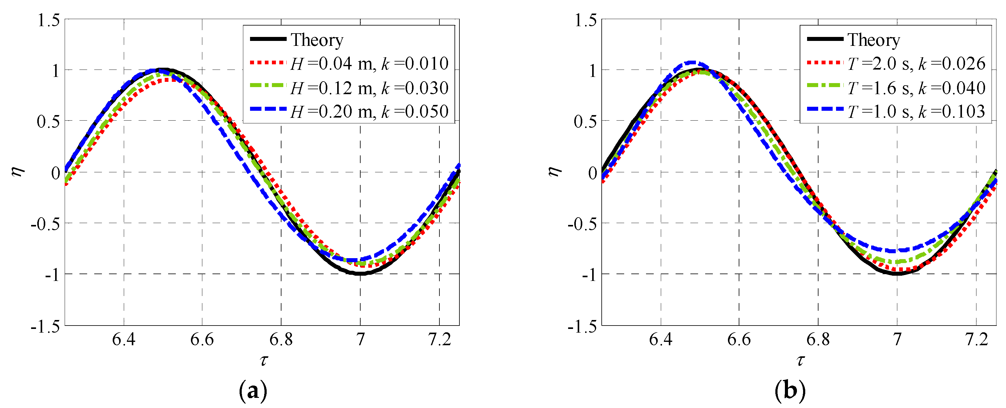
Figure 13 shows the non-dimensional free surface elevation,
η = 2
h/
H, where
h denotes the free surface elevation, and
H denotes the wave height, as a function of the non-dimensional flow time for different wave steepness at
T = 1.6 s and
H = 0.16 m, respectively. When looking into
Figure 13, it can be found that: with the increase of wave steepness, the wave crest becomes shaper and the wave trough becomes flatter. This process is similar to the transient process from the Airy wave to the second order Stokes wave, indicating that the nonlinearity of the wave increases with wave steepness.With the increase ofwave nonlinearity, the drift torque drives the Duck to capsize when the wave condition exceed a critical value. In this situation, since the Duck departures from its original equilibrium position, the comparison of the pitch angular displacement amplitude of the Duck between the CFD and BEM model will be meaningless. Therefore, a dashed line is shown in
Figure 12 to distinguish the useful data in the left part from the useless date in the right part.
The paragraphs above attributed the difference between the CFD and BEM model to hydrodynamic nonlinear factors, and the reason can be explained as follows. The BEM model is based on the Laplace Equation, which is originated from the Navier-Stokes Equation with the assumptions of inviscid fluid, incompressible and irrotational flow. To solve the Laplace Equation, the linear wave theory, which assumes that both the wave steepness and motion response of the WEC are small, is employed. On the other hand, the CFD model used in this work is based on the RANS Equation, which is also originated from the Navier-Stokes Equation but with the turbulence effect be approximated by empirical models. Although both two models adopt approximations, the CFD model is closer to real flow conditions than the BEM model since the fluid can be viscid, and the flow can be compressible and rotational. With the increase of wave steepness, large wave steepness may violate basic assumptions of the linear wave theory, resulting in the BEM model loss the ability to accurately predict the hydrodynamic response of the WEC. Therefore, the CFD model is expected to be more accurate than the BEM model in this case.
5.5. Vortex Generation Processat the End of the Duck
In the above section, we inferred that one of the hydrodynamic nonlinear factors is from the Duck motion, which is mainly embodied by the vortex generation phenomenon around the Duck, especially at the end the Duck. In this section, we try to study the vortex generation process around the WEC using the validated CFD model. For the solo Duck WEC, the vortex generation process is a new challenge since it does not appear for the spine-connected Duck since there are almost no gaps between the Ducks. The pressure difference between the blocked flow in the front area of the Duck and free flow at the end causes vortexes to be generated, which is also very common in aerodynamic design of airplane wings [
34] and wind turbine blades [
35], where blade tip losses are caused by pressure differences. The flow passing the end of a Duck is similar to a steady flow passing an obstacle with leading and trailing rectangular corners, as shown in
Figure 14. In the upstream, the blockage of the obstacle causes a vertical velocity component of the flow in the front area of the obstacle. At the leading corner, the sharply deceleration of the vertical velocity in the vertical wall boundary layer causes an advert pressure gradient leading to flow separation. Under the compression of the main stream, the separation zone is restricted to a limited zone, and reattachment of the boundary layer happens when the horizontal wall is suitably long. At the trailing corner, the same phenomenon appears since the horizontal boundary layer reaches another corner, and this will cause another flow separation. In both the upstream and downstream positions, standing vortexes are generated and denoted as P and Q, respectively. Because a rectangular angle is the infinite approximation of a sufficiently large curvature, the leading and trailing corners act as the fixed flow separation points for the geometry. These vortex generation phenomena are extensively studied in [
36,
37,
38,
39]. The direction of P and Q is perpendicular to plane of the main flow with the polarity be determined so that the peripheral velocity of the vortex follows the main flow.
Figure 15 shows the fluid velocity and vorticity distribution around the end of the Duck at
T = 1.6 s and
H = 0.12 m. In the left column, the subfigures show the approximately undisturbed fluid velocity vector distribution in the plane
y = 2.4 m. The hollow circle represents the rotation axis of the pitch motion. Within a wave period, as shown in the linear wave theory, the velocity direction of water particles at a fixed point is of circular type, as shown in
Figure 15i and the time sequence follows the clockwise principle as A→B→C→D→A. In the right column, vorticitydistributionof the main vortexes are shown in either the free surface, i.e.,
z = 0 plane, or the perpendicular surface, i.e.,
x= 0 plane. Since the peripheral velocity of the Duck is small relative to the fluid velocity, the Duck can be considered as standing still in the flow field. At time instance A, the main flow is in the
x-y plane, i.e.,
z = 0 plane. As illustrated in
Figure 14, the main vortexes will be generated in the
z direction. The P type vortex is generated at the leading cornerat the end, while the Q type vortex is at the trailing corner, and the direction of these vortexes are both positive so that the peripheral velocity of the vortices follows the main flow, and this is confirmed in
Figure 15b.
At time instance B, the main flow is in the
y-
z plane, i.e.,
x = 0. Similar to the above principle, the P and Q vortexes are generated and both in the positive
x direction as confirmed in
Figure 15d. At time instance C, the situation is rightly opposite to time instance A. The location of P and Q vortexes are reversed, and both are in the negative
z direction as shown in
Figure 15f. At time instance D, both location and direction of P and Q vortexes are reversed from time instance B as confirmed in
Figure 15h.
From above discussions, we find that: at different time instances within a wave period, the magnitude and direction of the generated vortexes are different, and vary periodically. Vortexes are generated due to the relative motion between the WEC and the fluid, thus part of the kinetic energy of the WEC will be devoted to feed the vortex generation process, resulting in the captured power of the WEC be reduced.
The vortex generation process causes the static pressure in the downstream side of the obstacle be smaller than that of the upstream side, resulting in a force resisting the relative motion of the obstacle, e.g., a resisting torque for the Duck in this paper. This resisting force is called the drag force, whose magnitude is proportional to the square of the velocity and direction is opposite to the velocity. Therefore, the nonlinearity of the Duck motion, which is embodied by the vortex generation phenomenon, can be quantitatively represented by the drag torque. Besides, since the analysis in
Section 5.4 revealed that the nonlinearity of the wave is positively correlated to the nonlinearity of the Duck motion, we combine the two nonlinear factors together so that the total nonlinearity is quantitatively represented by a single drag torque. As in [
40], the drag torque of the Duck in the pitch degree-of-freedom can be defined as:
where
Cd is the drag torque coefficient. Then, according to the Newton’s Second Law, we can obtain the equation of motion of the Duck as:
where
Te is the excitation torque,
Tr is the radiation torque, and
Th is the hydrostatic torque. By solving Equation (9), we can obtain the motion response of the Duck in the time domain considering the drag torque. However, the drag torque coefficient in Equation (8) for a given wave condition cannot be obtained directly. In this paper, this drag torque coefficient is obtained in an indirect way as in [
33], by tuning its value until the motion response of the Duck obtained from Equation (9) equals that of the CFD model.
Figure 16 shows the drag torque coefficient as a function of wave height at
T = 1.6 s and
c = 12 N·m·s/rad. At small wave heights, the drag torque coefficient is almost zero. However, at large wave heights, the drag torque coefficient increases significantly with wave height. This is due to the nonlinear behavior of the wave and the vortex generation phenomenon is more prominent at large wave heights. The observed variation tendency in
Figure 16 indicates that the drag torque coefficient effectively reflected the influence of the nonlinearity of the wave and the Duck motion. This gives the opportunity to build a database of the drag torque coefficient as a function of wave height, wave period, etc, so that the hydrodynamic nonlinearity can be modeled with reasonable accuracy without the time-consuming CFD model.
5.6. Hydrodynamic Force Distribution Along the Longitudinal Direction of the Duck
In order for the solo Duck WEC to survive in harsh offshore climates, the hydrodynamic force distribution along the longitudinal direction of the Duck should be carefully considered in designing the intensity and stiffness of the WEC structure.
Figure 17 shows the comparison of surge and heave forces per unit square meter along the longitudinal direction of the Duck among 3D CFD, pseudo 3D CFD and BEM results at
t = 8.544 s when
T = 1.6 s and
H = 0.08 m.
The pseudo 3D CFD simulation is intended for simulating the hydrodynamic performance of the spine-connected Duck, and is implemented by applying the symmetric boundary at both ends of the Duck. Correspondingly, 3D CFD and BEM simulations are performed for the solo Duck. The hydrodynamic forces keep almost constant in the longitudinal direction in pseudo 3D CFD simulations, while vary continuously in 3D CFD and the BEM simulations, as a result of the diffracted and radiated wave in the
y direction, which cannot be developed in pseudo 3D CFD simulations. This indicates that the structure design of the solo Duck should be different from that of the spine-connected Duck when considering the longitudinal force distribution. In both 3D CFD and BEM simulations, when approaching the end of Duck, the surge force decreases, while the heave force gradually increases. One interesting finding in both subfigures is the rapid jump of the forces at the end of the Duck in 3D CFD simulations, and is quite remarkable for the heave force.
Figure 18 shows the comparison of the dynamic pressure contour between 3D CFD and pseudo 3D CFD simulations at
t = 8.544 s, when
T = 1.6 s and
H = 0.075 m. It can be seen that the position where dynamic pressure dramatically varies, which is not observed in pseudo 3D CFD simulations, coincides with where vortexes are generated. Actually, the vortex generation process is due to pressure differences around the end of the Duck. The pressure near the end of the Duck quickly drops down since the vortexes take away the kinetic energy from the fluid, resulting in the rapid jump of the pressure force. The comparison shows that the CFD model can subtly capture the local feature of the vortex generation process and its influence on the hydrodynamic forces. Therefore, the CFD model is recommended for this kind of calculation. From the above discussion, it is found that the hydrodynamic forces of the solo Duck are different from that of its spine-connected counterpart. The resultant surge force of the solo Duck is smaller than the spine-connected Duck, which means that the modulus of the Duck cross section in the
x direction can be reduced, and furthermore, the mooring force in this direction can also be reduced. Meanwhile, the resultant heave force of the solo Duck is also smaller, which means that the modulus of the Duck section in the
z direction can be reduced, and likewise for the mooring force. Overall, the smaller dynamic surge and heave forces will reduce the fatigue load on the Duck WEC hull and the mooring system, which will result in the fatigue life of the Duck to be extended.


