1. Introduction
Distributed generators (DGs) based on green-energy technologies are strongly promoted in governmental and industrial policies around in the world, due to agreements that promote the decrement of energy generation using fossil fuels [
1,
2]. Wind turbines, solar panels, and storage systems are the most promising technologies [
3,
4] to reduce the use of fossil fuels. Particularly, micro-grids are considered to be the key in future electric grids based on renewable energy, since a micro-grid groups DGs, storage systems, and loads in clusters to make the control and management of DGs easier [
5]. DGs based on renewable energy resources are denominated inverter-interfaced units because a power converter is employed to tie the DG to the grid. As inverter-interfaced units, such as solar panels and storage systems, are non-synchronous generators, they lack rotational inertia, causing large frequency variations which affect the stability of the grid [
6]. An useful alternative to alleviate instability is the addition of virtual inertia in the control scheme—namely, virtual synchronous generator (VSG) schemes—include artificial inertia in the control loop through the integration of a swing equation to emulate the rotational inertia of synchronous power generators [
7].
DGs using the VSG scheme have been widely studied because they are capable to work in island and grid-connected modes [
8]; however, their stability analysis and control design are studied under balanced conditions. Additionally, DGs with VSG working in grid-connected mode are sensitive to grid disturbances, such as low voltage ride through (LVRT) and voltage sags [
9,
10]. Control schemes for DGs with virtual inertia dealing with unbalanced conditions are presented in [
9,
10,
11,
12], but the proposed control algorithms are linear proportional-integral-derivative (PID-type) algorithms, which present sensitivity to model variations [
13,
14].
Additionally, non-linear control techniques have been applied to DGs with the VSG scheme. In [
15], a non-linear control algorithm was designed using a large signal model (non-linear), then the performance of VSG was tested with parameter variations; however, unbalanced conditions were not considered. Back-stepping control, as well as sliding mode control, were applied to VSG in [
16]; despite the verified stability of the control scheme, the performance of the controller was only tested considering transitions from island to connected mode. Intelligent control techniques, such as neuronal networks and fuzzy logic control, were presented in [
17,
18], where the controllers were tested under disturbances (inertial variations), and different power commands, but unbalanced conditions were not verified. Therefore, robust control strategies for DGs based on renewable energy technologies are required: They must be capable of addressing lack of inertia and sensitivity against parameter variations, as well as unbalanced conditions.
Fuzzy logic control (FLC) can address the problem of model variations, as its design does not require the use of mathematical models; it transforms human knowledge into a non-linear mapping [
19], which defines the control input to be applied, in accordance to defined if-then rules. Naturally-inspired computing has been applied to improve the performance of FLC systems by means of the use of meta-heuristic optimization methods, social communication techniques, chemical structure-based learning algorithms, and so on [
20]. Particularly, artificial hydrocarbon networks (AHN) provide a useful computational algorithm for control and modeling problems [
21]. Stability, robustness, and accuracy are the main characteristics of AHN [
21] because it is a chemically inspired technique, based on carbon networks, which catches stability in the topology of the algorithm and partial knowledge of the system behavior [
20]. Thus, control algorithms with AHN are capable of dealing with uncertain, imprecise, and noisy data [
22]. The efficacy of AHN control systems is supported by its application in a position controller of the two-axes tool in a computer numerical control (CNC) for high-precision machines [
23], a liquid-level controller in a coupled-tanks system [
24], and a controller for a doubly-fed induction generator wind turbine [
22], among others.
In this paper, a robust control scheme for DGs operating under unbalanced conditions is proposed. The presented scheme is composed of an AHN controller to regulate reactive power while an active power loop maintains the conventional topology of the VSG to preserve inertia. Thus, the contributions of this paper can be summarized as:
A robust control scheme capable of regulating reactive power, where inertia is included through the VSG scheme to preserve stability; and
A control scheme able to accomplish robust power regulation, as it works under voltage-unbalanced conditions, which is the main drawback of DGs with VSG. Furthermore, the robustness is preserved during changes from connected to island mode, and vice versa.
The properties of the control scheme based on AHN are validated by simulations considering one- and three-phase voltage sags.
The structure of the paper is as follows: The control scheme is presented in
Section 2; the bases of AHN are given in
Section 3; the proposed robust control scheme is proposed in
Section 4; and the simulations are shown in
Section 5.
2. Problem Statement
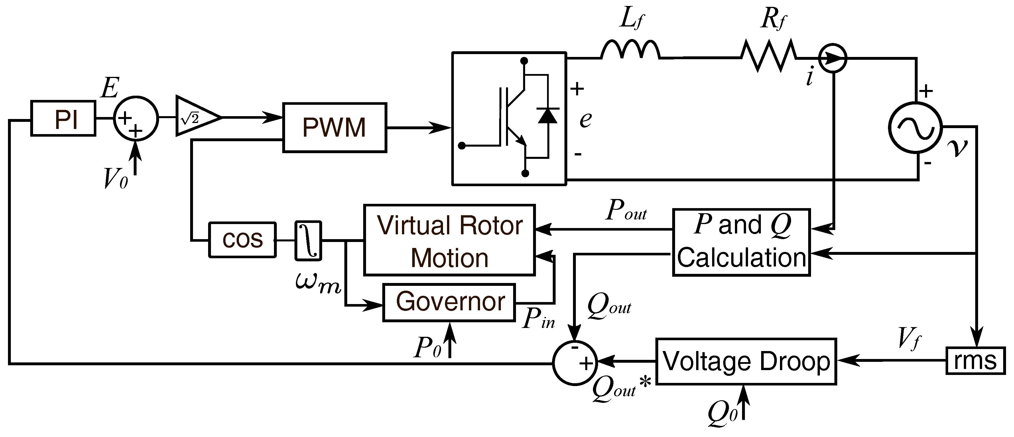
Consider the control scheme presented in
Figure 1, which is widely employed to include virtual inertia in DGs [
7]. Reactive
Q and active
P power control loops are part of the scheme, both in a
reference frame. The
P loop contains the following elements [
25]. The active power calculation,
where
,
,
, and
are the currents and voltages in the inverter terminal on a
rotating reference frame. Then,
and
are computed as
where
represents
or
.
The rotor swing equation
where
is the virtual rotor angular frequency,
J the inertia, and the block named governor represents a droop characteristic, defined as in [
6],
where
is the nominal angular frequency,
is the droop coefficient, and
is a given set active power.
On the other hand, the
Q loop contains the next elements [
25]. The reactive power calculation block consists of
The voltage droop block generates the reference of reactive power
, and is computed as
where
is given set reactive power,
is a reference of voltage,
is the droop coefficient, and
is the voltage rms of the filter output. The reactive power controller is
where
is the transfer function of a proportional-integral (PI) controller.
The relation between inverter output current, terminal voltage, and inverter side voltage is represented by the dynamics of the filter inductor [
26],
where
,
,
, and
are the currents and voltages in the inverter terminal,
and
are the inverter side voltages,
is nominal frequency (generator), and
and
are inductance and resistance of filter’s inductor.
Taking into account the equations of the control scheme in
Figure 1 ((
1)–(
8)), one can note the following issues:
This paper proposes a robust control algorithm to tackle the aforementioned issues. The proposed scheme is capable of compensating for model variations and disturbances due to unbalanced conditions while inertia is maintained.
In the next section, the basis of AHN is presented to understand the robust control algorithm given later.
3. Artificial Hydrocarbon Networks
An artificial hydrocarbon network (AHN) is a supervised learning method capable of extracting information from and to model data, which is inspired by chemical hydrocarbon compounds [
21]. The basic units of AHN are carbon and hydrogen molecules (CH-molecules), and each CH-molecule produces an output response
associated to an input
x [
20],
where
is the carbon value,
are the hydrogen values (i.e., hydrogen atoms attached to the carbon atom), and
k is the degree of freedom in the molecule. Two or more CH-molecules can be grouped to form an AHN-component, named an artificial hydrocarbon compound, which is described as follows,
where
is the behavior of the compound,
are the molecular behaviors, and
are the bounds of the molecules (i.e., the limits of the output response of each molecule produced by input
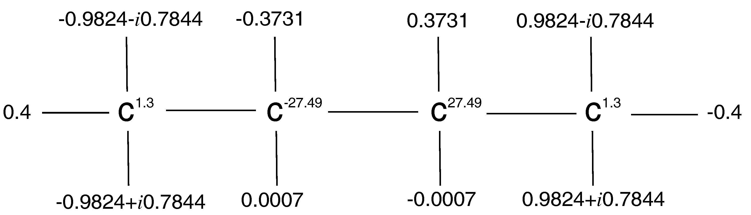
x). A particular structural representation of an artificial hydrocarbon compound is
where
n is the number CH-molecules (i.e., molecular behaviors). Details about an optimal algorithm to compute the distance between molecules was presented in [
20]. Thus, an AHN is a combination of artificial hydrocarbon compounds useful to predict, to model, and to classify data based on chemical rules [
22].
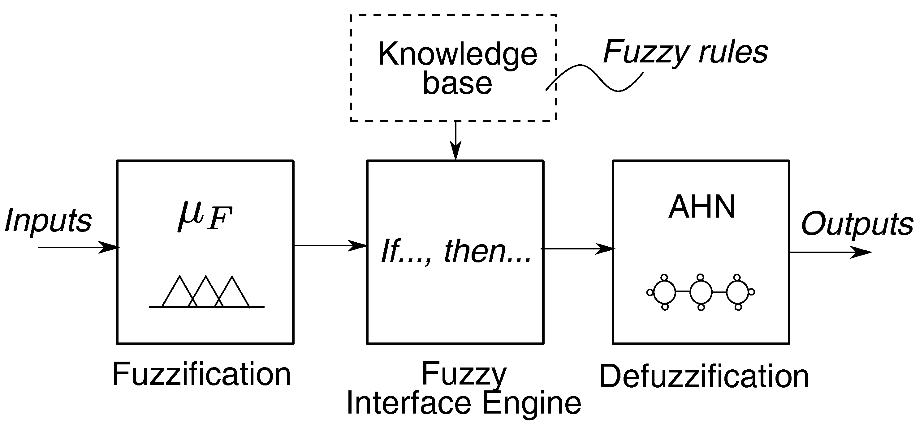
3.1. Fuzzy-Molecular Interface Systems
The block diagram in
Figure 2 describes a fuzzy-molecular interface system, which consists of three steps [
21]: Fuzzification, the fuzzy inference engine, and molecular de-fuzzification (i.e., a de-fuzzification process using AHN). Fuzzification consists of mapping the input
x to a fuzzy value
by means of a fuzzy set and its membership function,
The fuzzy inference engine consists of the evaluation of antecedents in terms of fuzzy rules:
where
is the molecular behavior of the
CH-molecule (
) of the AHN, and
is computed as
Then, the consequent value
is obtained as
Finally, in the defuzzification stage, the crisp value of
y is computed as
The knowledge base is a matrix that summarizes the fuzzy rules presented in (
13), considering the combination of all input variables
, and the molecules
. Assuming the rules
an example of this matrix is presented in
Table 1.
The advantages of the fuzzy model interface are [
21]: The fuzzy partitions in the output domain might be seen as linguistic units (for example, “low” and “high”); fuzzy partitions have a degree of understanding (the parameters are metadata); and molecular units deal with noise and uncertainties.
3.2. AHN Controller
A control algorithm that executes its control effort using a fuzzy-molecular interface system is known as AHN controller [
22], which is able to deal with uncertain and noisy data. Moreover, the design of AHN controllers is easy, because CH-molecules integrate expert and real-data information in single units.
The detailed control scheme for DG using an AHN controller is presented in the next section.
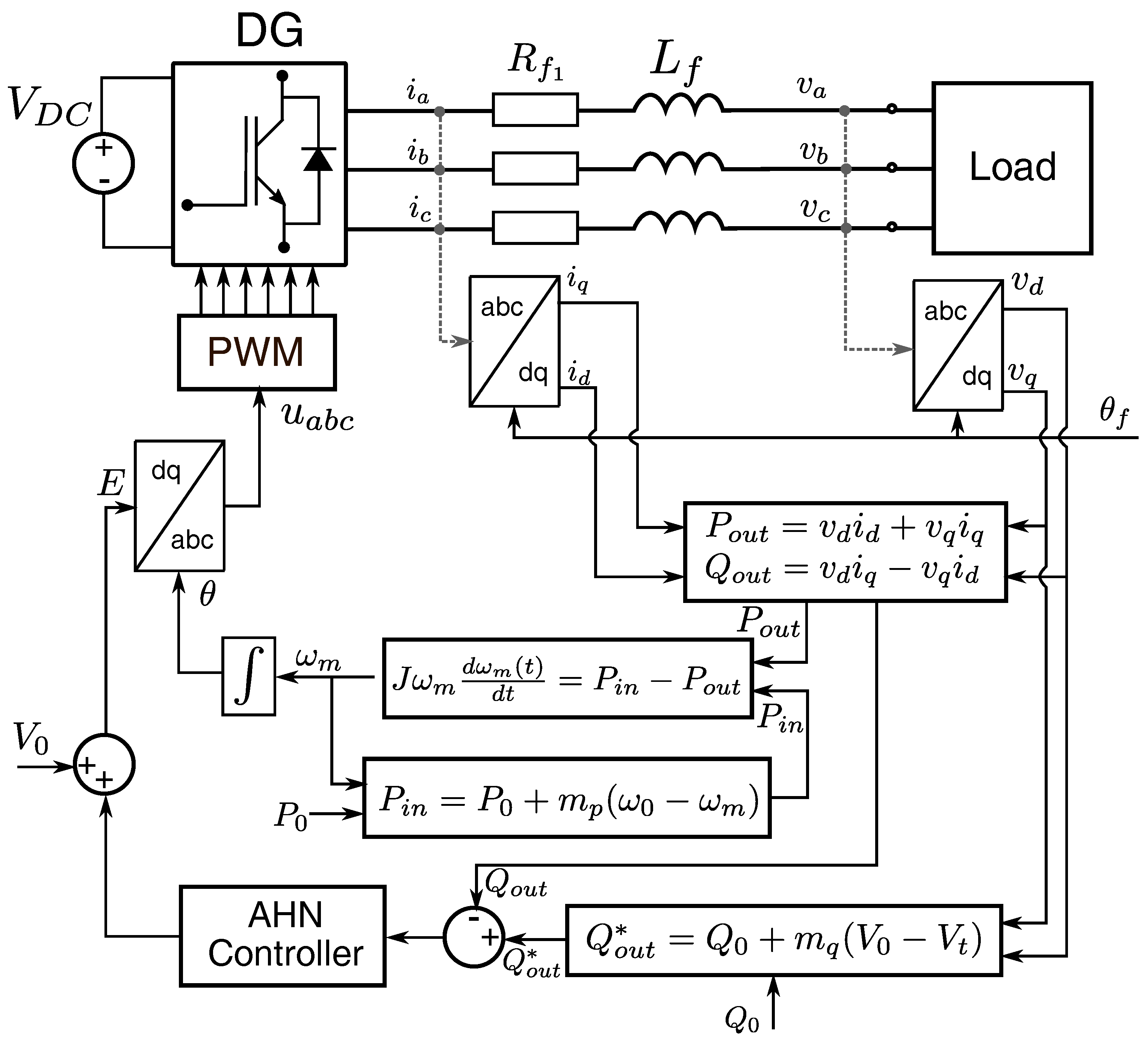
4. Robust Control Scheme Using AHN
Figure 3 presents the diagram of the proposed robust control scheme, where two control loops can be identified: The first one, related to the active power
P regulation (
P-loop) and the second one with reactive power
Q regulation (
Q-loop).
P and
Q are computed using the
components with angular position
, where
is the rotational frequency of the
frame. The P-loop contains the virtual inertia necessary to suppress frequency oscillations, which is preserved as in the conventional VSG scheme. The Q-loop integrates an AHN controller, instead of the conventional PI control (see
Figure 1), to provide a robust regulation of reactive power. In this section, the design of the robust AHN controller is presented.
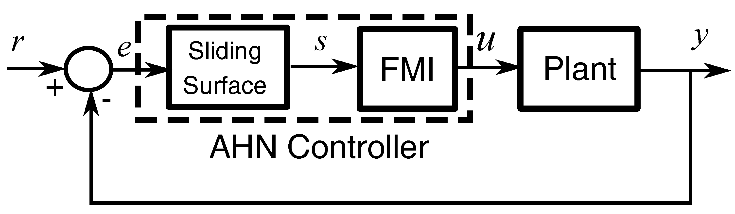
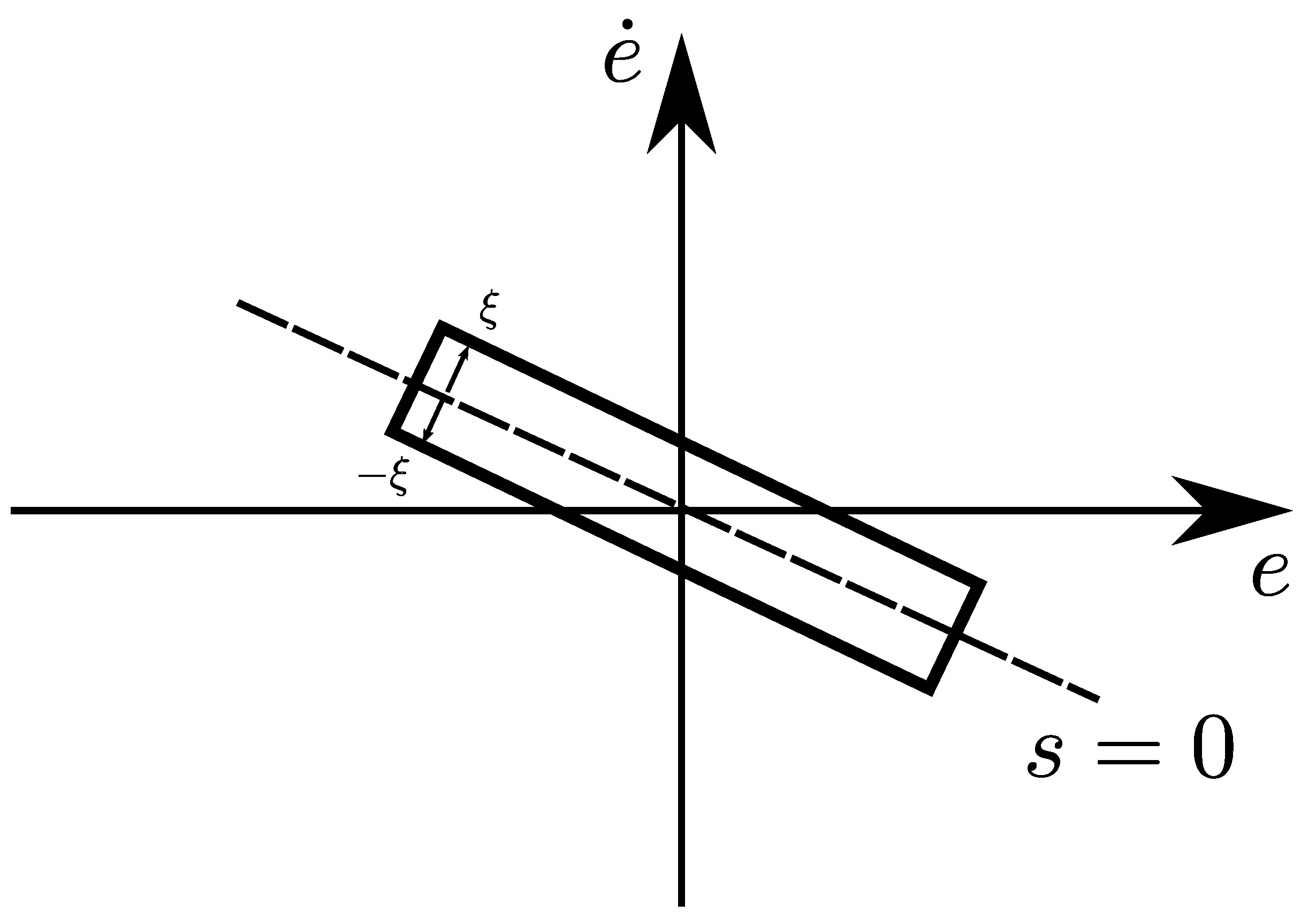
The proposed AHN controller is composed of a fuzzy sliding surface in a feedback loop with a fuzzy-molecular interface system, see
Figure 4.
The fuzzy sliding surface is defined as
where
is a constant and
e is the regulation error. The state-space representation of
s is shown in
Figure 5 [
27]. Thus, the AHN controller does not response to changes in the regulation error
e or its derivatives, but it reacts to changes in
s; therefore, the number of fuzzy rules is reduced compared with classical fuzzy logic control.
The rules to be implemented in the fuzzy-molecular interface of the AHN controller are as follows:
where NB, NM, ZR, PM, and PB mean negative big, negative medium, zero, positive medium, and positive big, respectively. Note that the objective of the fuzzy-molecular interface is to keep
; thus, if
, the dynamics of the system driven by the AHN controller is reduced to
, which has a solution
. Therefore, when
, the regulation error
e converges asymptotically to zero, and does not depends on the parameter of the system to be controlled.
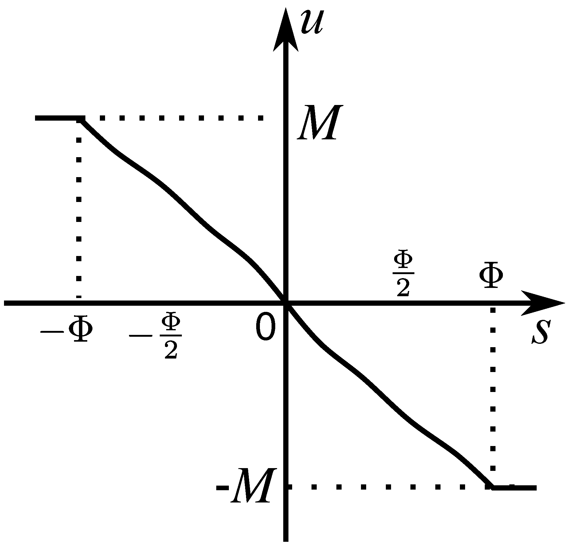
The output of the fuzzy-molecular interface results in the control input presented in
Figure 6, which can be represented as [
27]
where
M is the maximum value of the control gain and sigm is the sigmoid function, defined by
Note that function (
20) is similar to the AHN-component in Equation (
10), then a CH-molecular representation can be obtained, as in Equation (
11). Moreover, the form of AHN control is similar to a saturation function. The computation of gain
M and the test of stability of the AHN controller are presented in the next subsection.
4.1. Design of AHN Controller for DG
Define the tracking error of reactive power
Q as
where
is the reactive power reference and
is the reactive power measured from inverter output. Consider the Lyapunov function [
28]
where
, and whose derivative,
, is
Assuming balance conditions and
constant, the reactive power is defined by Equation (
5) and
, then
Adding Equation (
8) into Equation (
24), and assuming the derivatives
(since the inverter output voltages
,
are constants, see Equation (
2)), we obtain
where
is the nominal angular frequency,
, and
u is the control input to be designed. Defining
and replacing it in Equation (
25), one gets
where
is the disturbance term. Choosing
with
, and considering
,
is rewritten as
Therefore, selecting ensures that the trajectories converge to , despite the presence of a disturbance , and the tracking error e is asymptotically stable.
4.2. Design for Unbalanced Conditions
Negative sequence components emerge in the DG scheme when the grid voltage is unbalanced. The reactive power under unbalanced conditions is computed as [
11,
29],
where
and
represent the voltage/currents of positive and negative sequences, respectively. Note that the zero sequence components are not studied in Equation (
28), which does not represent a weakness for application since three-phase, three-wire unbalanced systems require the use of a negative sequence.
Including Equation (
28) into Equation (
25), the derivative,
, is
where
and
are the negative sequence reactive and active power, respectively; and the disturbance term is
. Then, the derivative of
V, considering the perturbed dynamics for reactive
, can be rewritten as
where
is a disturbance composed of the unbalance voltage terms (i.e., sequence negative components), as well as active power terms. Then, choosing
with
, the gain
M must be selected as
, where
isthe upper bound of disturbance
. Note that parameter variations, such as
, can be included in the disturbance term
; therefore, the selection of a control gain
also ensures robustness against parameter variations.
As the term
is a discontinuous term, which causes high frequency oscillations in the control system, the function sign is replaced by the sigmoid function defined by Equation (
20) and
Figure 6. As has been validated in [
27,
28], the controller
with a sigmoid function, as in
Figure 6, is a boundary-layer controller, which presents the robustness verified by the Lyapunov analysis using the function in Equation (
22).
Therefore, the design of the proposed AHN controller consists of the following steps:
Define the fuzzy sliding variable as ;
Design the fuzzy-molecular interface in
Figure 2 with the rules in (
18);
Select the value of M using the inequality to compensate disturbances contained in ; and
Implement the control law with .
Note that the design of the AHN controller has the following advantages: Employing less membership functions, since the rules are defined with respect to the fuzzy sliding surface instead of the error and its derivatives (as in conventional fuzzy logic control); and robustness against bounded coupled disturbances, because M considers the disturbed system.
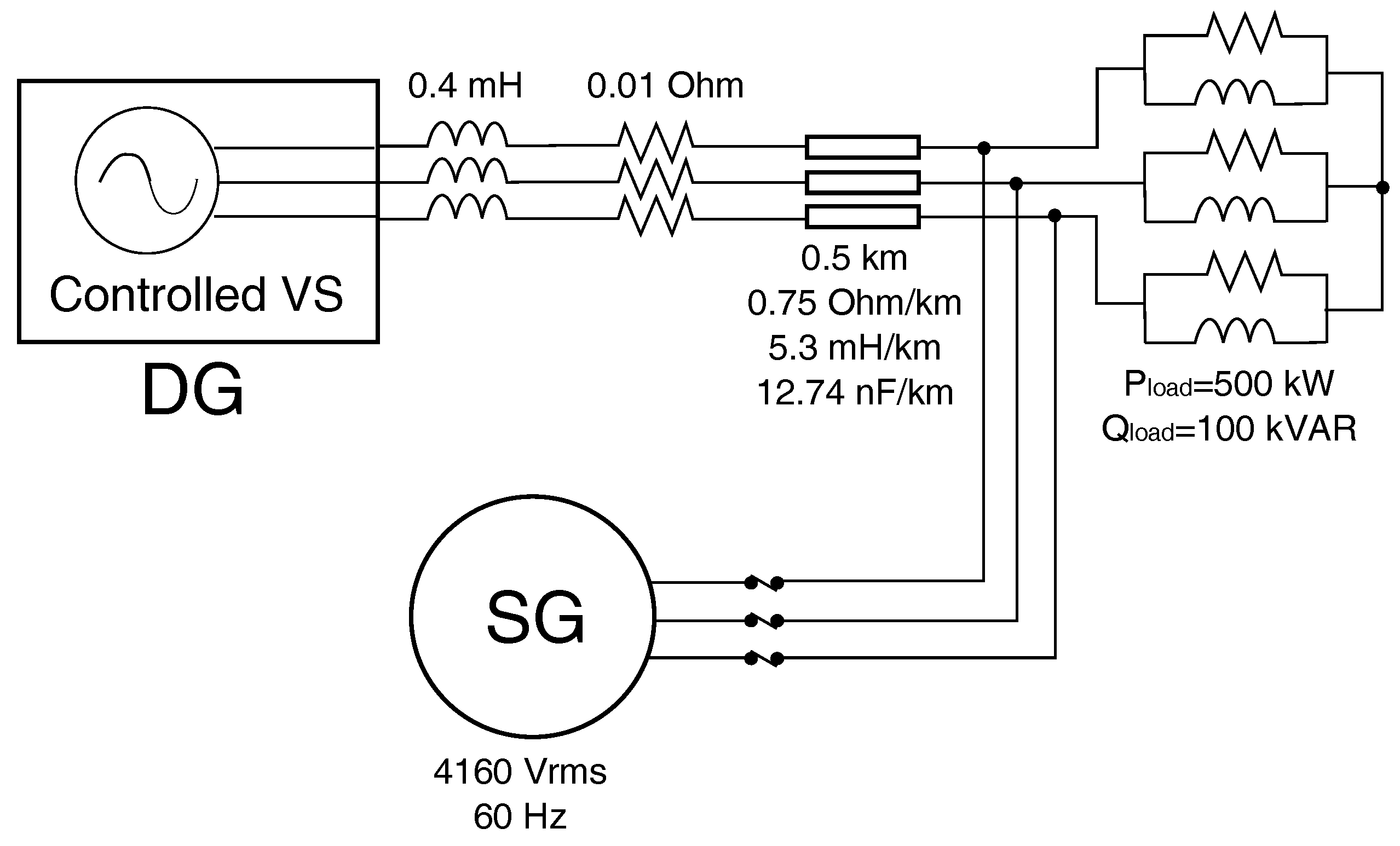
5. Simulation Results
In order to validate the proposed control scheme, the circuit presented in
Figure 7 is implemented in Matlab-Simulink (2018a, MathWorks, Natick, MA, USA), where the block named DG (Distributed Generator) contains the scheme of
Figure 3, which regulates the controller voltage source (VS), and the parameters of the
filter and loads. The parameters of the VSG Equations (
1)–(
6) are as follows:
,
, and
.
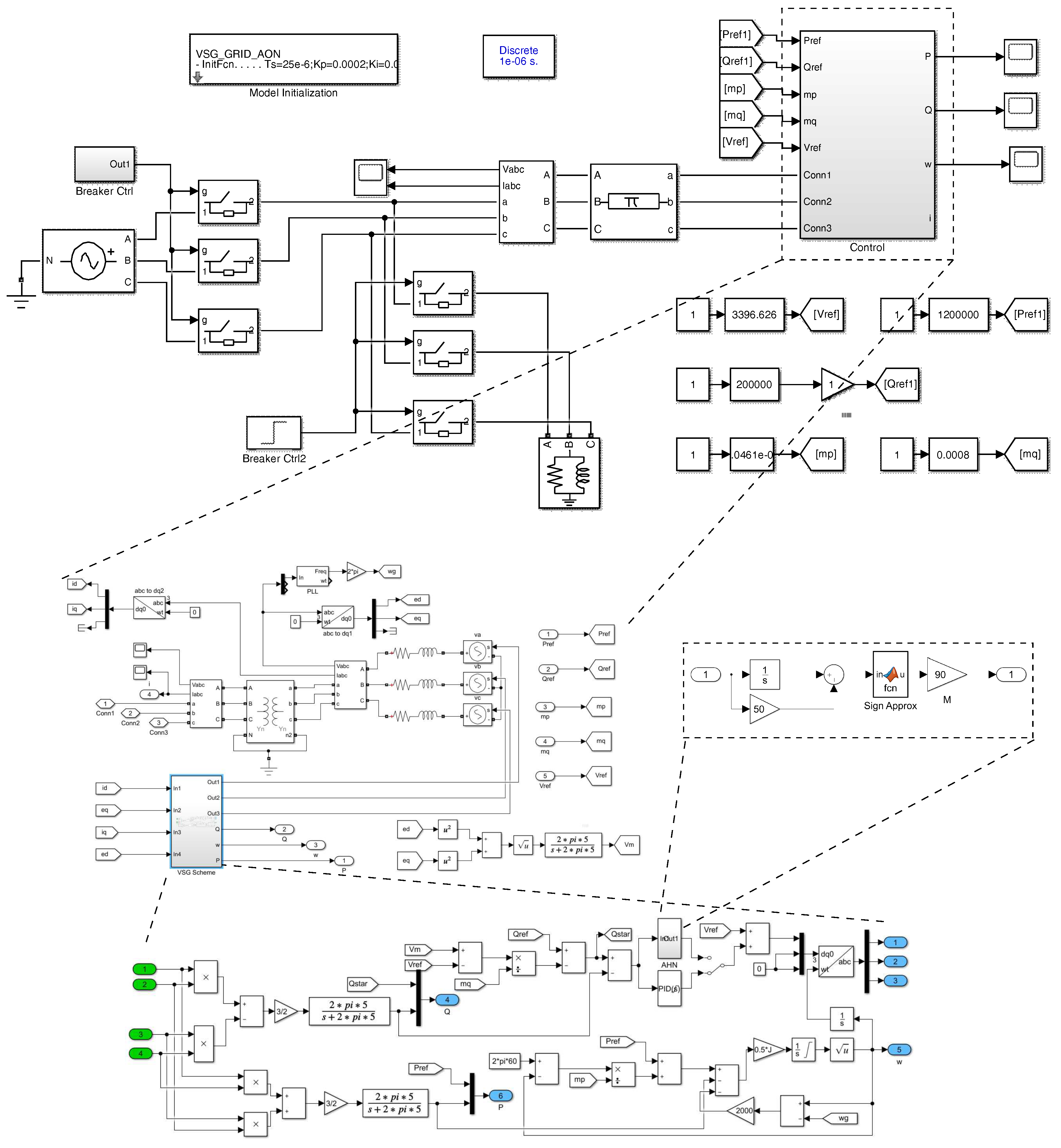
Figure 8 shows the Simulink blocks used for the simulation.
The fuzzy sliding variable is selected as
. The designed fuzzy-molecular interface is the following:
which has the structure presented in
Figure 9, and has control gain
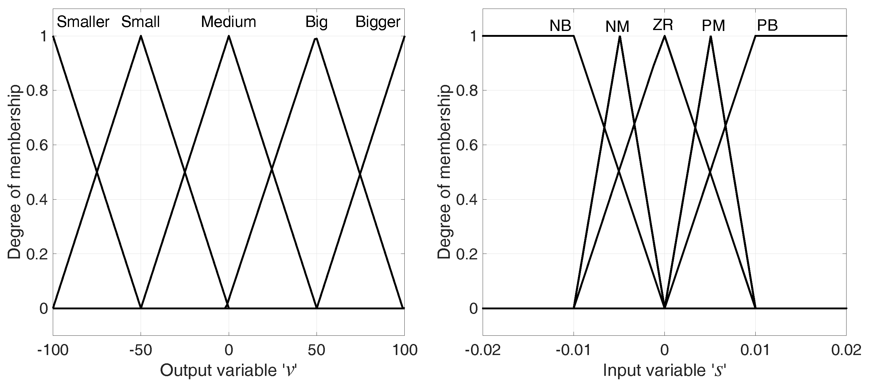
. The membership functions of the AHN are presented in
Figure 10.
The simulation conditions are the following: Simulation time is 5 s; fixed step size of 1 s; and the solver is ode1 (Euler). The unbalance voltage conditions are emulated by means of voltage sags (i.e., a decrement in the voltage amplitude of the synchronous generator). All the analyzed voltage sags are decremented from 1 p.u to 0.9 p.u in the voltage amplitude. In order to compare the performance of the proposed control scheme, a PI controller, with gains and , is also implemented. The PI gains are tuned considering the same reach time, from initial conditions to reactive power reference, as the AHN controller.
Three simulation tests are presented considering
MW,
kVAr, and the parameters of the circuit of
Figure 7. The control objective is to regulate active and reactive power at
MW and reference
in Equation (
6). The first test considers a voltage sag, in phase ‘a’, at time
s, which is maintained until
s; the second test is executed under same conditions as test one, but the voltage sag is applied in the three phases, ‘a’, ‘b’, and ‘c’; and the third test presents the transition between grid-connected and island modes, where
1–3 s is grid-connected mode, and island mode is maintained from
3–4 s. Finally, at
4 s, grid-connected mode is activated again.
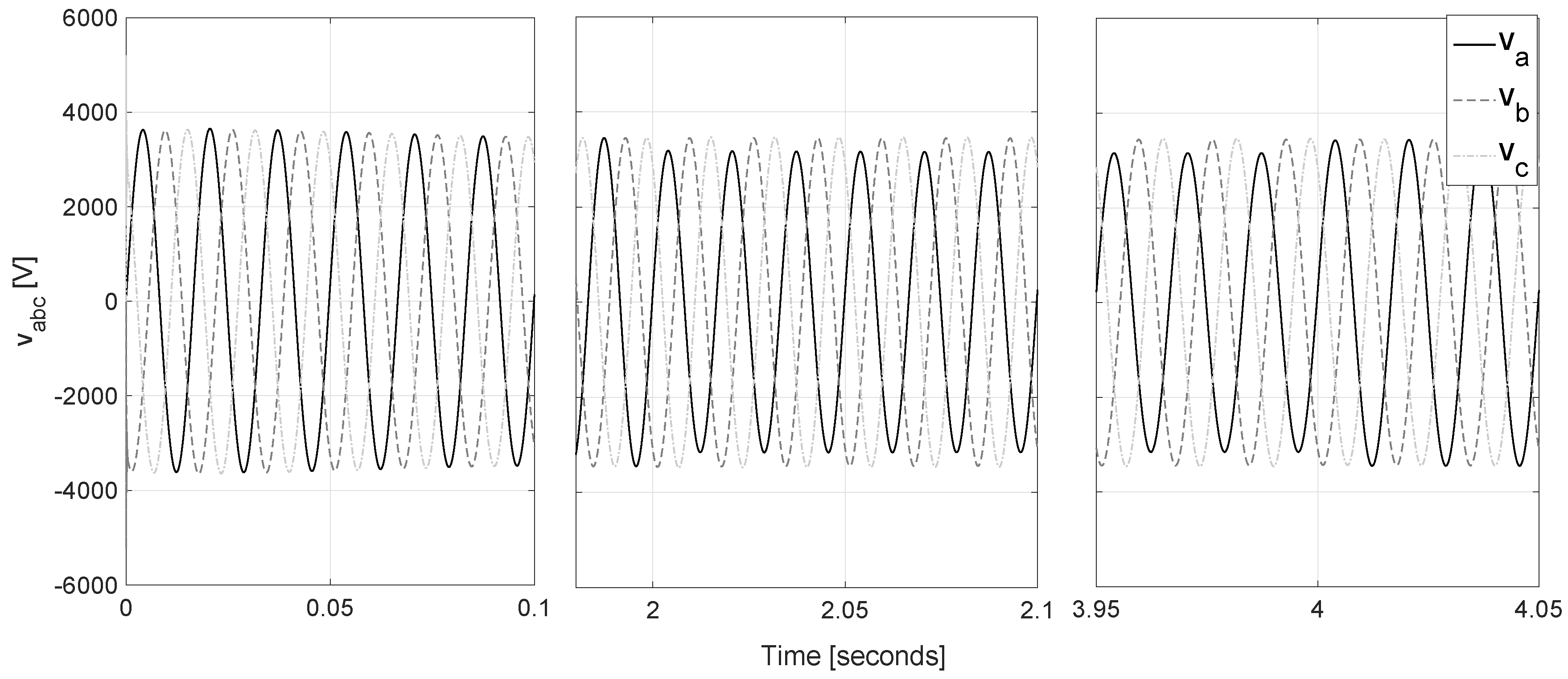
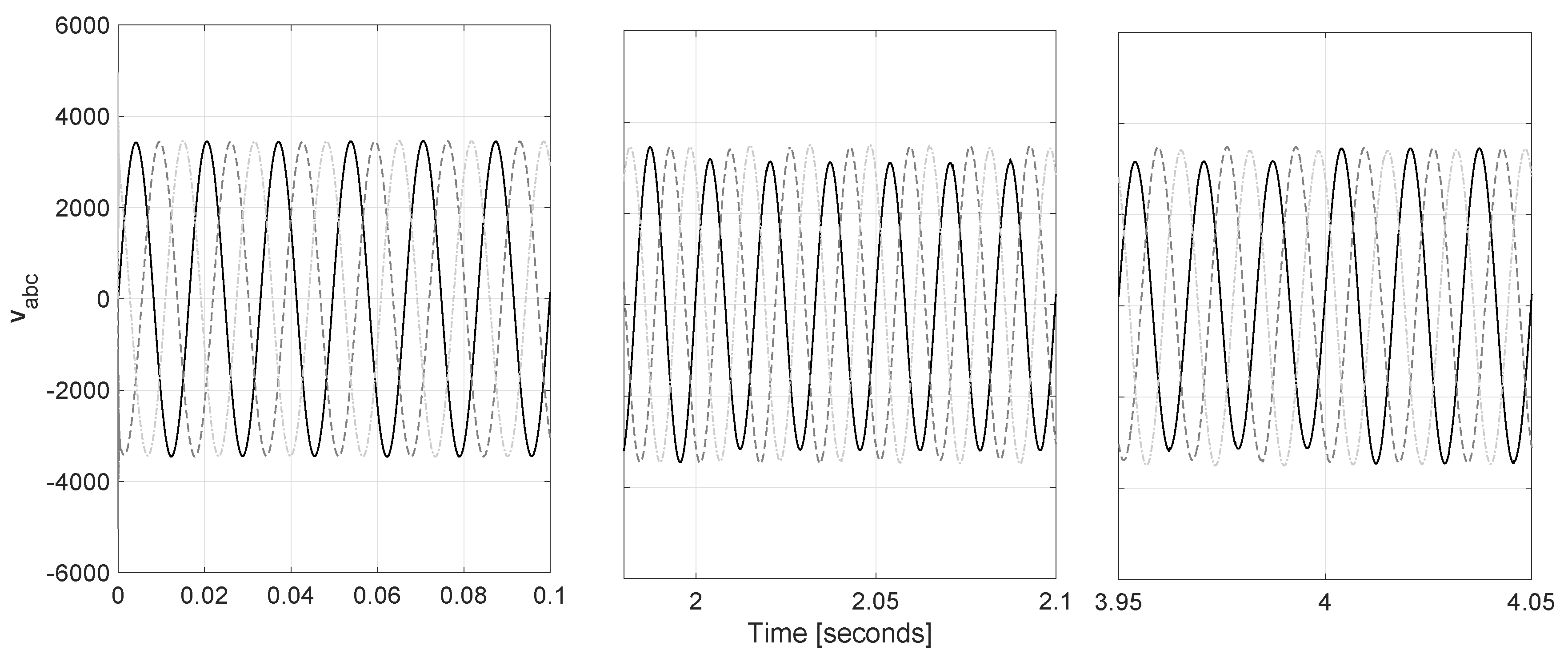
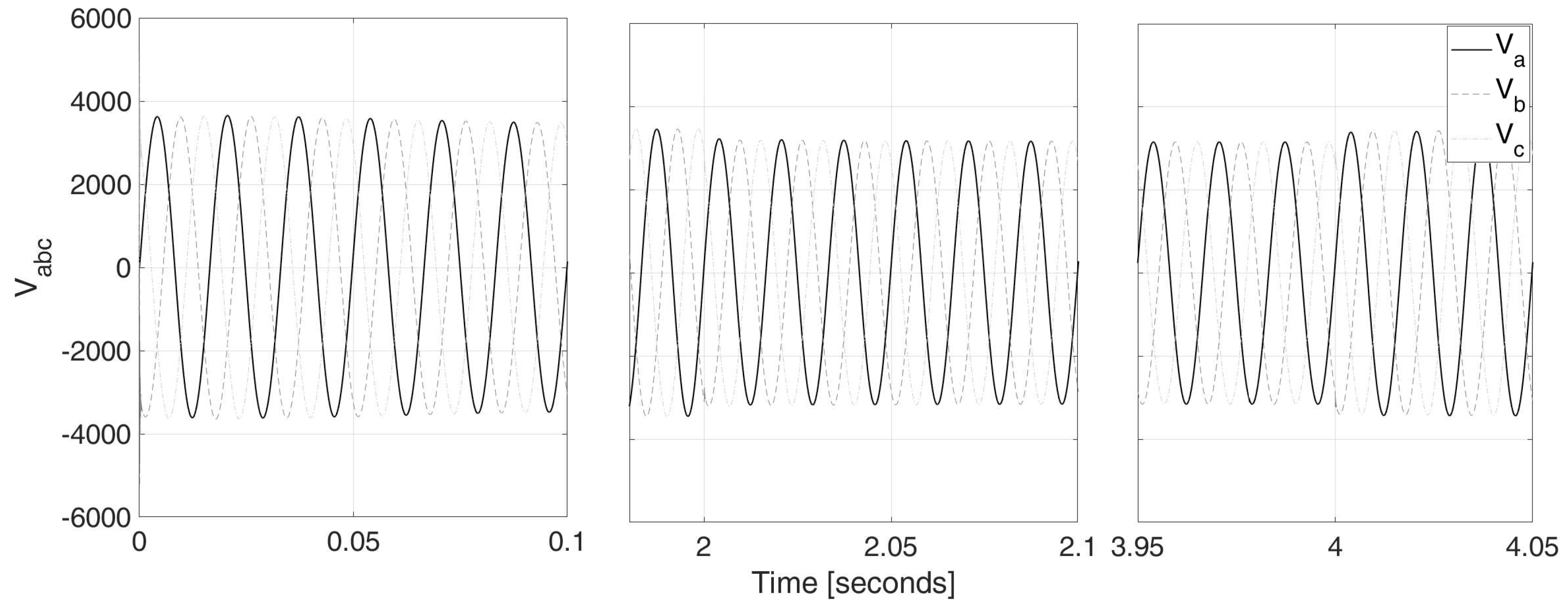
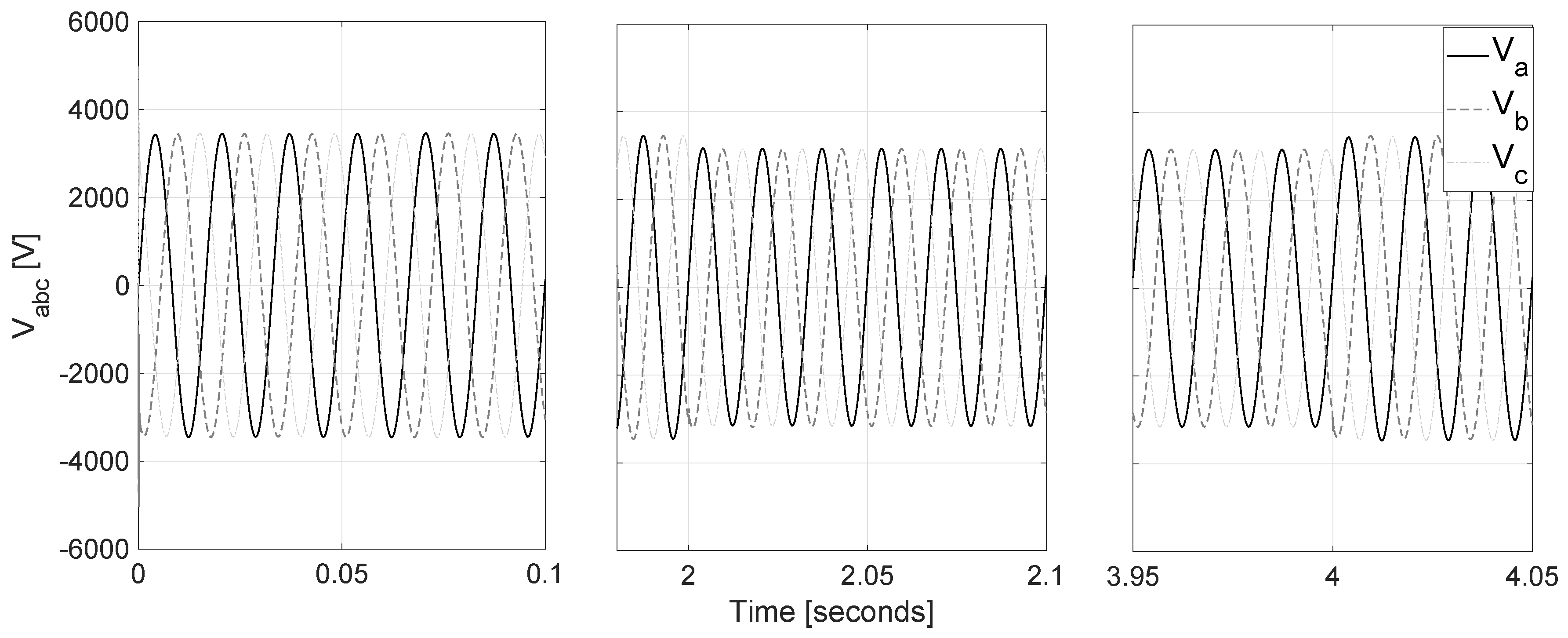
The voltages
for Tests 1 and 2 are presented in
Figure 11,
Figure 12,
Figure 13 and
Figure 14, respectively. The voltages sag at 2 s and where it is removed at 4 s can be observed.
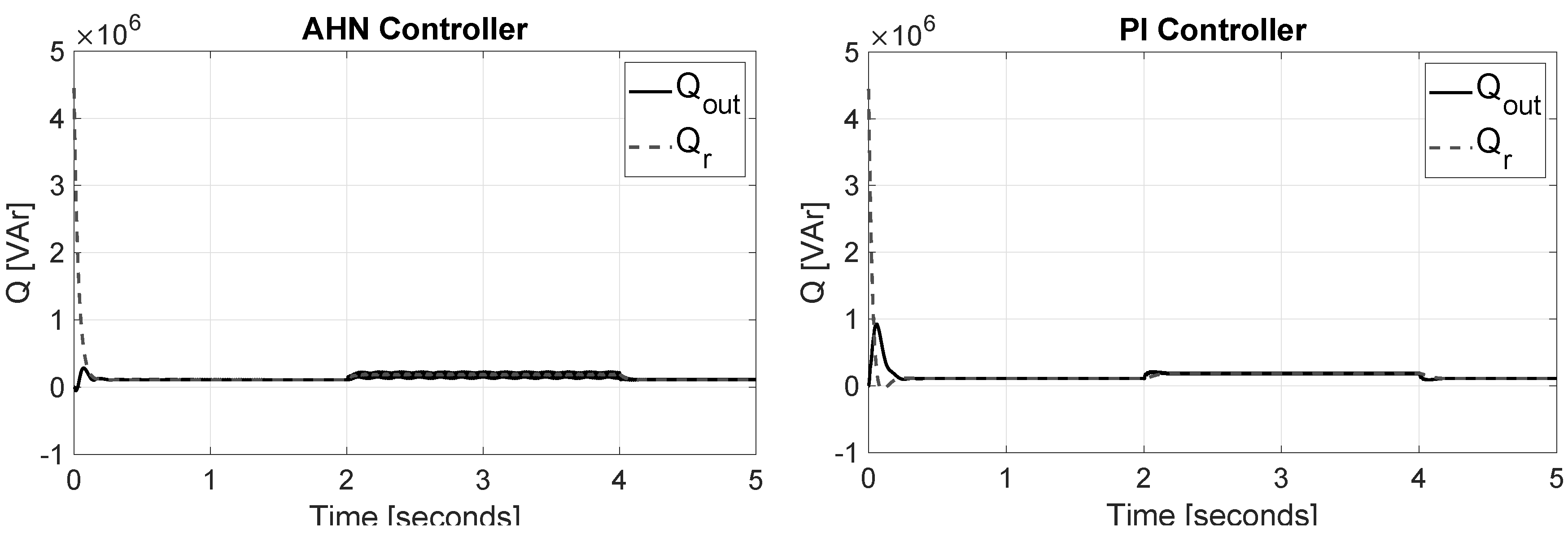
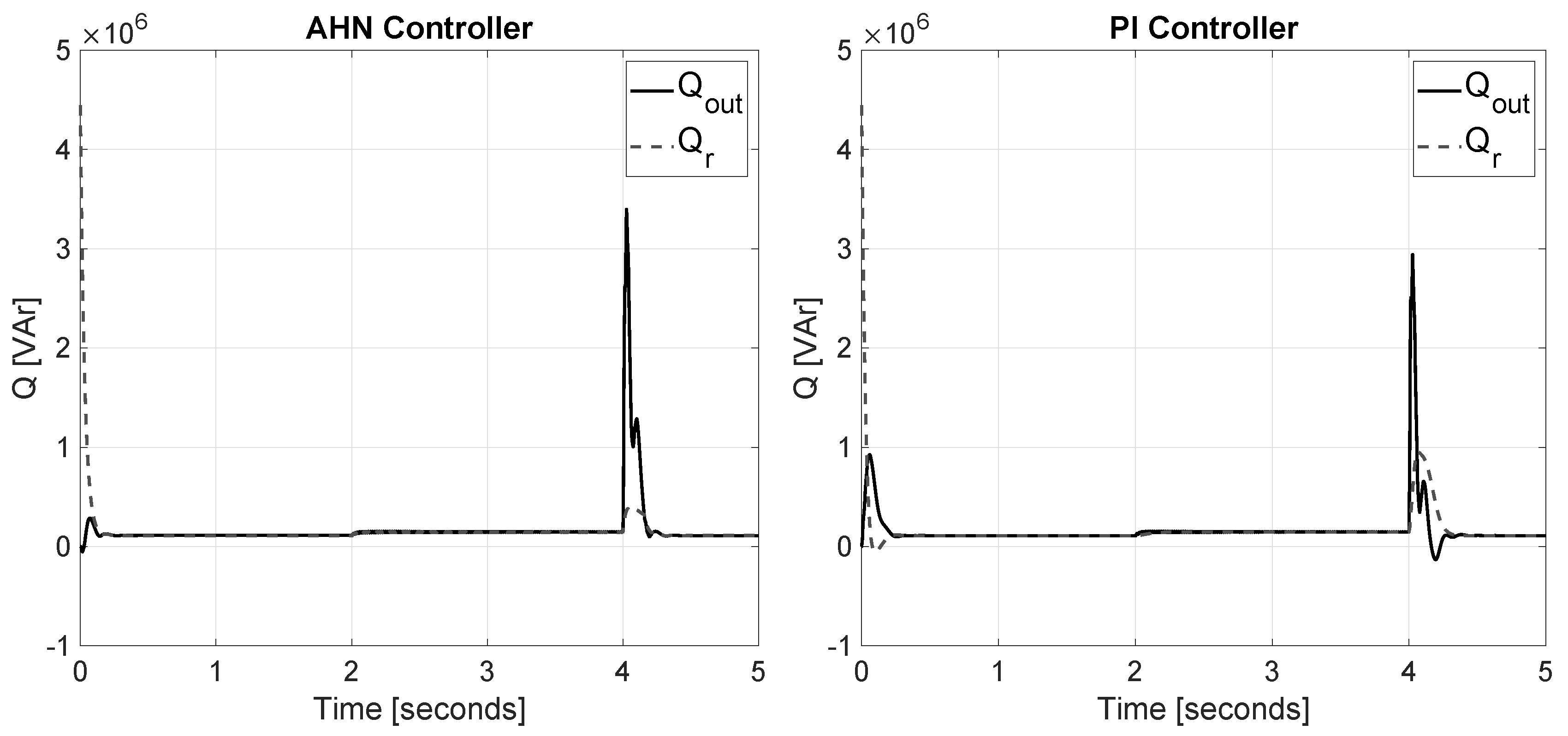
The simulation results of Test 1 are presented in
Figure 15, for the system with the AHN controller and PI. Reactive regulation is accomplished with both controllers, despite the effect of the voltage sag at
s. However, the transient response of the system with PI presents a overshoot five times bigger than the system with AHN controller.
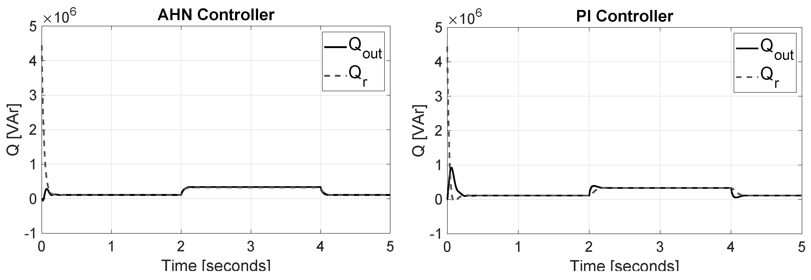
For Test 2, the results are presented in
Figure 16. Voltage sag emerges in the three phases at
s, where it can be seen that (similar to the one-phase sag test) the proposed AHN controller ensures reactive power regulation with a lesser overshoot than PI control.
Test 3, with a transition between grid-connected and island modes and vice versa, is presented in
Figure 17. One can observed that the transient response with AHN controller is still better than PI, since the overshoot is minor.
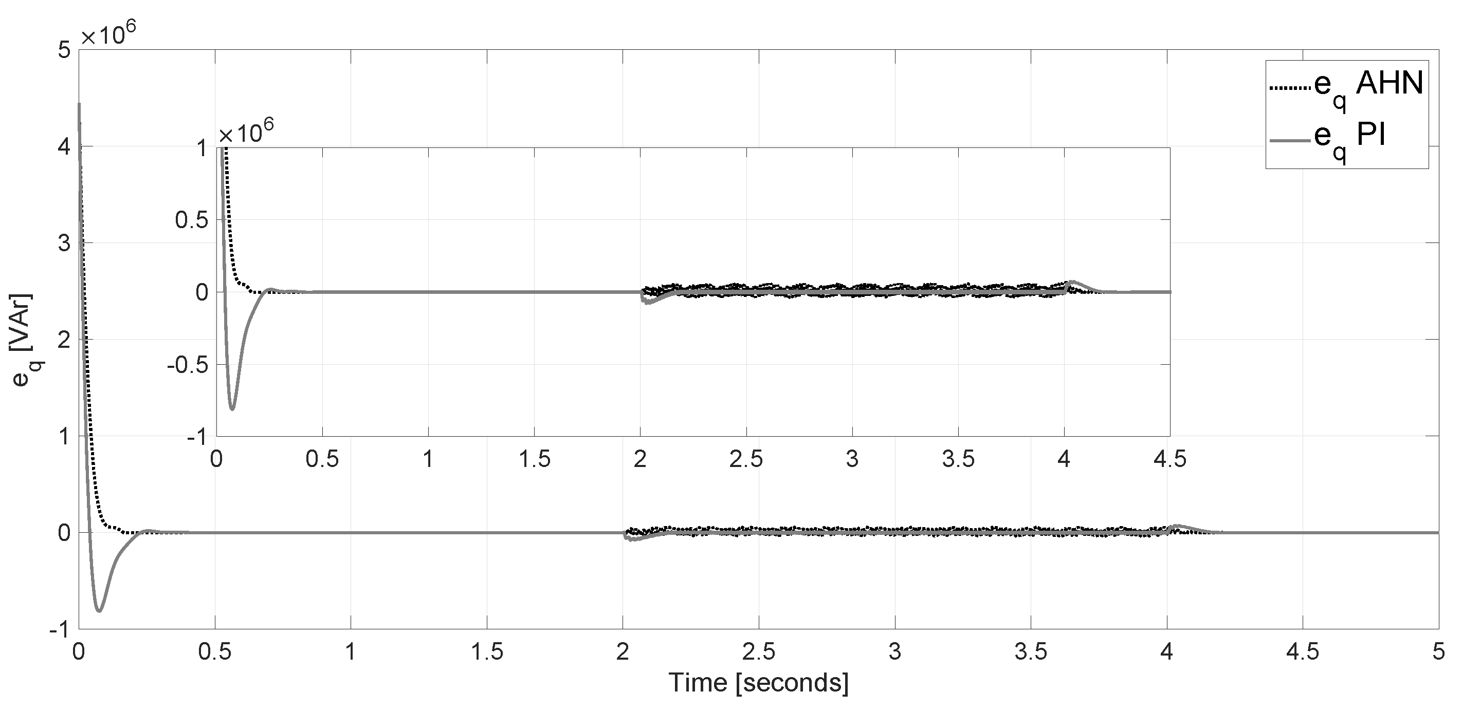
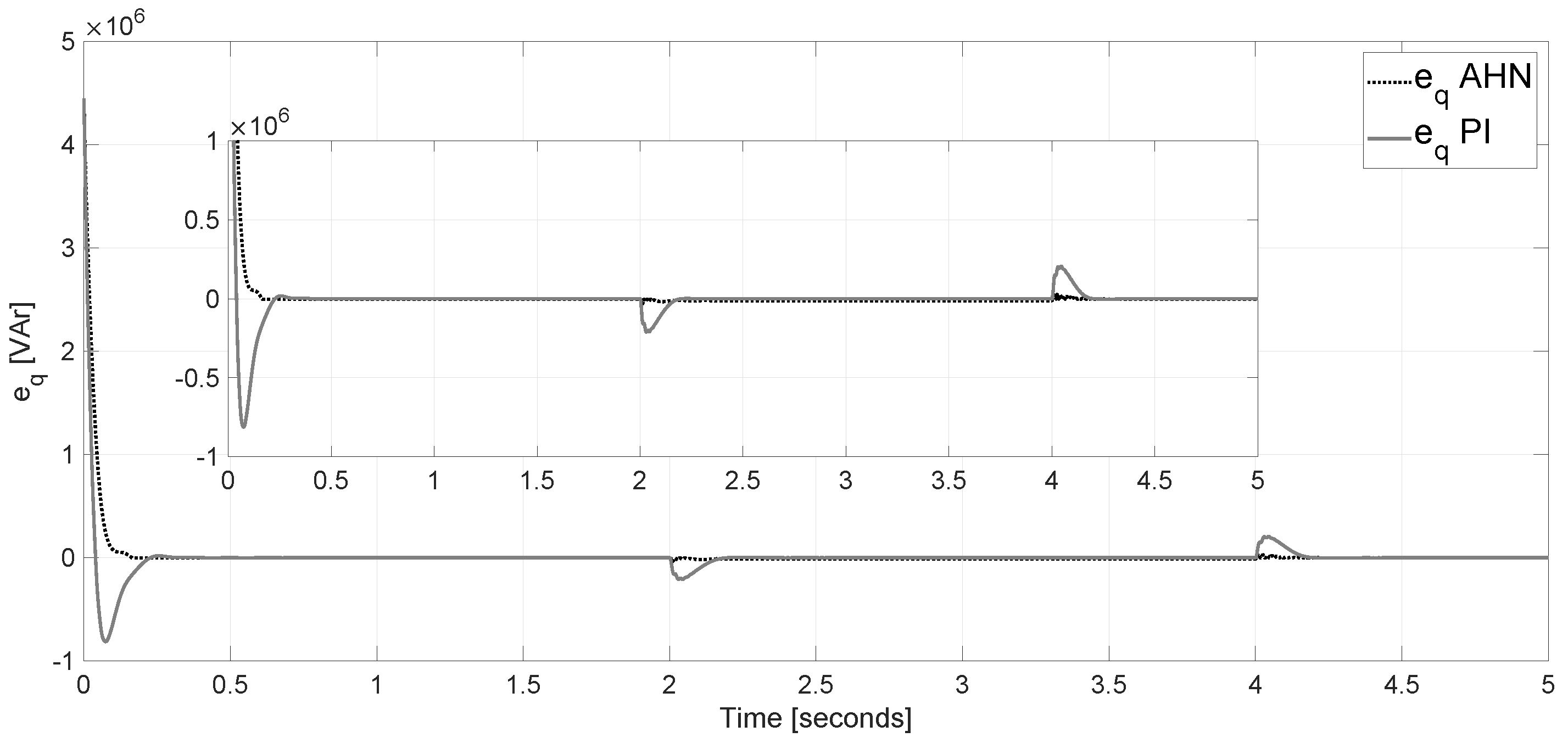
The regulation error,
, for Tests 1–3, are presented in
Figure 18,
Figure 19 and
Figure 20, respectively. One can observe that, during the changes resulting from the transition (0.5–1 s) and the voltage sags, the proposed AHN controller maintained a regulation error closer to zero, when compared with the PI controller. When the voltage sag appeared (disappeared) at 2 s (4 s), the PI control was not capable of regulating the reactive power in the reference, and
moved away from zero; see
Figure 18 and
Figure 19. Additionally, when the DG was reconnected to the grid during Test 3 (see
Figure 20), the system with PI control could not maintain the error closer to zero as the AHN control did. Thus, the proposed AHN is robust to voltage sags.
Table 2 and
Table 3 present a comparison between the AHN controller and PI for Tests 1–3, with respect to regulation error and control effort, respectively.
Table 2 considers the integral absolute error (IAE), computed as
, where
e is the regulation error. The control energy presented in
Table 3 is computed as
, where
u is the control signal. It can be observed that the error of the AHN controller is similar than PI control. However, if the control effort in
Table 3 is considered, the energy required by the PI control to reach a similar error to the AHN controller is at least two times larger.


