1. Introduction
In the past, only a few large power plants, mainly running on fossil or nuclear fuels, were responsible for the reliable supply of electricity [
1]. The continuous expansion of renewable energy sources enables a more sustainable design of the electricity system [
2]. At the same time, however, new challenges are emerging [
3]. The main challenge is the fluctuating electricity production caused by the weather dependency of wind turbines and photovoltaic plants, which make up a large proportion of renewable energy sources. Moreover, due to the merit order effect, renewable energy sources successively replace conventional power plants [
4]. These have so far provided most of the required flexibility [
4]. Thus, there is an increasing need for flexibility in the power system to keep ensuring the necessary balance between power generation and consumption. This is called the flexibility gap [
5]. In particular, flexibility can address the challenges caused by both foreseeable and unforeseeable fluctuations of renewable energy sources and therefore help to establish an environmentally friendly, decarbonized electricity system [
5,
6,
7].
Lund [
3] and Müller [
8] differentiate between four types of flexibility in the electricity system which guarantee security of supply: grid expansion, energy storage, flexibility on the supply side, and flexibility on the demand side. Here, flexibility on the demand side refers to the possibility of deviating from the planned load profile [
9]. Typically, such deviations are economically motivated by price signals. If a third party sends a signal to a flexible consumer, this is called demand response (DR) [
9]. Due to high costs for storage systems and grid expansion, flexibility on the demand side will play an important role as it offers flexibility at comparatively low marginal costs [
10,
11,
12].
The digital transformation of the electricity sector is opening up new opportunities for utilizing and automatizing the marketing of flexibility potentials [
13,
14]. For example, the use of smart meters enables improved monitoring and control of electricity consumption and therefore a higher automation level of flexible industrial production systems. Hence, the advancing digitalization on the one hand facilitates an efficient and repeated use of flexibility. On the other hand, it also provides digital communications technology to detect and react to local changes in power consumption in the electricity network, the so-called Smart Grid [
15]. With these tools at hand, it is possible to tackle the aforementioned flexibility gap from both the perspective of flexibility providers and from a systemic point of view [
12]. Since interoperability in a Smart Grid is an essential requirement, the uniform description and modeling of flexibility is of crucial importance for the optimal scheduling and successful use of flexibility [
16,
17]. The “Smart Grid Architecture Model” [
18] is a framework to support the development of the European Smart Grid. It consists of the following five layers: business layer, functional layer, information layer, communication layer, and component layer. The information layer is meant to provide a data model which ensures a common understanding of the exchanged data.
For an electricity system in which conventional power plants provide the main contribution to flexibility, typically a few key figures, such as activation duration (ramp up time), holding duration (length), and power (capacity) characterize a flexibility [
19]. However, as already mentioned, in the future electricity system, one will need new participants who provide flexibility [
5]. On the demand side, the industrial sector is of particular relevance as it consumes a large part of the electricity in many countries [
20]. Already today, some electricity-intensive companies are optimizing their power purchases, taking their available flexibility potential and price fluctuations into account. However, due to various barriers, such as know-how, or technical, economic, environmental, regulatory, and organizational challenges, many industrial companies have not yet exploited their DR potential [
5,
8,
21]. Standardization can improve the exchange of information and foster access to flexibility-related services. Therefore, it can contribute to a substantial decrease of these barriers, in particular these related to know-how, technical, and economic challenges. In this context, a standardized modelling of flexibility, which can be implemented by a generic data model, takes on an essential part [
14]. Such a data model should facilitate the description of any flexibility as precisely as possible on the basis of various key figures. At the same time, it has to feature an adequate degree of generality in order to capture all kinds of flexibility providers.
Some contributions in literature already deal with the description of power-related flexibility. For example, Reference [
22] designed a taxonomy for modeling flexibility. In order to characterize different types of flexibility, the authors defined the taxonomy “buckets”, “battery”, and “bakery”. These types exhibit various key figures such as power states, energy capacity, energy level at a specific deadline, and minimum runtime. In [
23], the authors developed a clustering of flexibility into four groups: load curtailment, load shifting, onsite generation, and utilizing electricity storage systems. Each group is described by various constraints. Based on that, the authors derived a decision-making model for DR aggregators in wholesale electricity markets. However, those forms of flexibility have been modeled in a simplified way and a precise description of the flexibility of industrial processes is not possible with this approach. Additionally, the authors use different key figures for each cluster, making the model rather unwieldy. Finally, based on an in-depth literature review, Reference [
24] presents a more generic approach in their work. They define a catalog of features whose generic optimization models must take into account to describe all possible kinds of flexibility (see
Section 6). However, our work in a major German research project shows that also this catalog and in particular its implementation exhibit several shortcomings. The following three aspects outline the contribution of our work:
We propose a generic data model which we developed in the course of a major German research project to model power-related flexibility. The modular structure of the data model allows us to precisely describe different types of flexibility.
The data model allows transferability among different sectors and hence provides an opportunity for standardization. It therefore constitutes a basis for integrating flexibility into information systems and thus improved information exchange and a higher automation level. This allows for automating the use of flexibility.
We validate our data model in close collaboration with companies from a major German research project. In the process, it has been demonstrated that the data model is suitable to represent flexibilities with different characteristics of the companies.
The focus of this article is on the description of generic power-related industrial flexibility, although our results are sufficiently generic to also apply to households [
25], small-scale industries, trade, services [
26], and supply side flexibility. Electric cars will also become increasingly important as novel participants in the electricity system [
27,
28]. The data model can also be applied to the charging and discharging of electric cars. Usually, flexibility exhibits one or more degrees of freedom and can therefore be regarded as a subset of a multi-dimensional space. In order to describe a specific instance of a flexibility, i.e., an element of this space, we also present a data model for what we will call flexibility measures.
The remainder of this paper is organized as follows. In
Section 2, we describe the research project in which we developed and validated our generic data model. Next, in
Section 3, we present the proposed data model for industrial flexibility by discussing the involved subcategories. In particular, we explain the need for and limitations of each of the subcategories’ key figures. In
Section 4, we then derive the corresponding data model for flexibility measures. Afterwards, we present how the data model can be used for different applications by means of two exemplary use cases in
Section 5. In
Section 6, a discussion compares our data model with existing work. Finally,
Section 7 summarizes the main findings and gives an outlook on future research.
3. Proposed Generic Flexibility Data Model
3.1. Heuristics
Modeling is generally a systematic abstraction of the real world. On the one hand, one has to describe the real world with sufficient accuracy. On the other hand, the model must be as simple as possible, in particular in case it is meant for practical applications. It is therefore necessary to make simplifying assumptions in the right places. After giving an overview of the subcategories of our data model (this Section), we will derive the corresponding key figures, explain why they are necessary, and discuss the underlying assumptions and simplifications in
Section 3.2,
Section 3.3 and
Section 3.4.
Our data model for flexibility contains components which can be chosen from three subcategories: flexible loads, dependencies, and storages. We define a
flexibility as a collection of such components. A flexibility has to contain at least one flexible load. It may, however, exhibit any number of dependencies and storages.
Figure 1 schematically visualizes the basic idea of the modular data model based on two exemplary flexibilities. Flexibility 1 exhibits three flexible loads. Moreover, flexible load 1a and 1b are interrelated by a dependency. The reader might consider the following illustrative example for such a constellation: a graphitizing oven exhibits two production phases which are represented by flexible load 1a and flexible load 1b. The second phase (flexible load 1b) always follows the first phase (flexible load 1a). The dependency then can describe that flexible load 1b requires the usage of flexible load 1a some time in advance. Flexible load 1c is an independent production machine, which at the same time exhibits flexibility. Flexibility 2, which can be associated with the same or another company, features two flexible loads, one dependency, and two storages. One storage is linked to two flexible loads, whereas the second storage is linked to only one flexible load. For instance, flexible load 2a and 2b can be two machines that manufacture the same product in different ways and store it in the product warehouse (storage 2a). Dependency 2 then accounts for the fact that the machines must not be operated simultaneously. Moreover, flexible load 2b utilizes the generated waste heat and stores it in a heat reservoir (storage 2b). As
Figure 1 illustrates, dependencies and storages always refer to flexible loads among the flexibility. In other words, a flexibility is a
closed object.
We regard a power-related flexibility as the opportunity to deviate from the original schedule with a resulting change in power consumption. Typically, a flexibility originates from one or more devices (units, machines). Such devices can exhibit different degrees of freedom regarding how they may operate, e.g., at different times or energy levels. We call the flexibility associated with an isolated device a
flexible load. Our modelling of a flexible load will be detailed in
Section 3.2. One can take into account the aforementioned degrees of freedom by representing each dimension by an associated key figure. A flexible load therefore parameterizes a set of individual load curves which can be realized by the flexible device. We call a single usage of a specific realization a
flexible load measure. It can be imagined as a specific choice from the range of each key figure of a flexible load. The corresponding key figures which describe the flexible load measure will be denoted in
italics with an attached asterisk (*). We will explain flexibility measures and flexible load measures in detail in
Section 4. Thus, a filled data model for a flexible load does in general not only contain numbers, but also subsets (ranges) of a corresponding basic set
. In other words, they are elements of the corresponding power sets
. Moreover, the key figures of a flexible load may have intrinsic interrelations. This means that not every key figure can be chosen freely from its associated base set. In other words, the choice of one key figure might restrict the accessible values for another key figure. For instance, some choices of key figures might be functions of the choices of other key figures within a flexible load measure and thus implicitly defined. Of course, we could in principle also define a separate flexible load for any combination of interrelated key figures. However, with the possibility of dependent key figures, the flexibilities can be defined more compactly and the partition of the process into flexible loads is more intuitive. In
Section 5, when we will have given a detailed explanation of the key figures, we will give illustrative examples for this property. Imagine that (ignoring units) the value of
key figure 1 may be chosen freely in the interval
and
key figure 2 (also ignoring units) always has to be twice the value of
key figure 1. Then, one would be tempted to write the following:
Since key figure 1 is given by a set, one would interpret the function as a set-valued function, the result being the image set of under f and hence . This would give the impression that the value of key figure 2, i.e., key figure 2*, may be chosen freely within the interval , which is clearly not what we intended. What we wanted to say is that for every flexible load measure specified by the corresponding flexible load, the functional relationship between the associated key figures must hold: ).
If there are several flexible loads involved in an industrial process, one might expect that one can represent this in our data model by simply moving to product spaces, i.e., arbitrary combinations, of flexible loads. However, we observed that, in reality, we cannot assume that a flexible load is always isolated. Consequently, similar to what we explained for intrinsic interrelations of key figures within a flexible load, also key figures from different flexible loads might be related. Thus, not all of the aforementioned product space is accessible. From our observations in SynErgie, we learned that it is usually sufficient to consider only logical interrelations among pairs of flexible loads. They are typically related to certain requirements on process sequences. We will call the subcategory which describes such interrelations
dependencies. A dependency thus connects key figures from the two involved flexible loads. This is achieved by defining suitable key figures for dependencies, which in turn refer to key figures of (measures of the) interdependent flexible loads. These will be described in detail in
Section 3.3.
Finally, we observed interrelations which can be clustered under the common term
storages. We will introduce storages in
Section 3.4. It is important to keep in mind that batteries are rather an exception in industrial processes. When thinking about storages, one should rather consider stocks for products in batch processes or reservoirs for heat, cold, or chemical products. Unlike dependencies, storages only pose constraints on the energy consumption of the flexible loads which they are connected to. In other words, the energy content of storage must satisfy certain bounds for all times. Moreover, in contrast to dependencies, storages can also cause costs.
As opposed to flexible loads, both dependencies and storages do not add any degrees of freedom to the flexibility. They pose boundary conditions which restrict the admissible combinations of flexible load measures among which we may choose or optimize in a subsequent step. This explains why we did not allow to define a flexibility which does not contain a flexible load: in this case, the flexibility space would be empty and could thus be ignored.
Figure 2 illustrates two flexible loads each of which are assumed to exhibit one degree of freedom. The respective degrees of freedom are depicted on the two axes. The flexible loads are further interconnected by a dependency as well as storage. Recall the above example where two machines (flexible loads) are connected by a dependency and supply storage. The degree of freedom results from
key figure 1 for both flexible load 1 and flexible load 2.
Figure 2 illustrates that flexible load 2 has more freedom than flexible load 1. The resulting black area in the middle is the remaining, accessible flexibility: Only certain combinations of measures of the two associated flexible loads are accessible. If there were no constraints involved, any combination of measures from flexible load 1 and 2, i.e., the whole rectangle, would be accessible. An optimization (with respect to a certain objective function) will then choose the “best” element among the (accessible) flexibility, i.e., a flexibility measure, which can then be executed.
In the following subsections of
Section 3, we define the key figures of the three subcategories flexible loads, dependencies, and storages.
3.2. Flexible Loads
Let us consider a non-empty planning horizon . One would imagine a planning horizon as a certain time interval, e.g., from 8:00 a.m. to 6:00 p.m. on a specific day. It is in general given by a subset of the reals. We decide that the unit is seconds, measured with respect to the common reference point 1 January 1970, which is—apart from units—close to what one would regard a date–time from a programming-oriented perspective. As already discussed, a flexible load describes the opportunity of an isolated device to deviate from the scheduled power consumption. Hence, it can bee seen as a family of maps which associate with every time t in the planning horizon the corresponding change in power consumption . Mathematically, we could consider any subset of , which denotes the set of all functions from to .
However, in SynErgie, we learned that, for practical purposes, this generality goes too far. In the following, the required key figures for a flexible load are derived from the findings in the project. It turned out quickly that it is not necessary to include arbitrarily complicated families of load curves
into our model. Rather, for applications, it is sufficient and more practical to restrict to families of maps
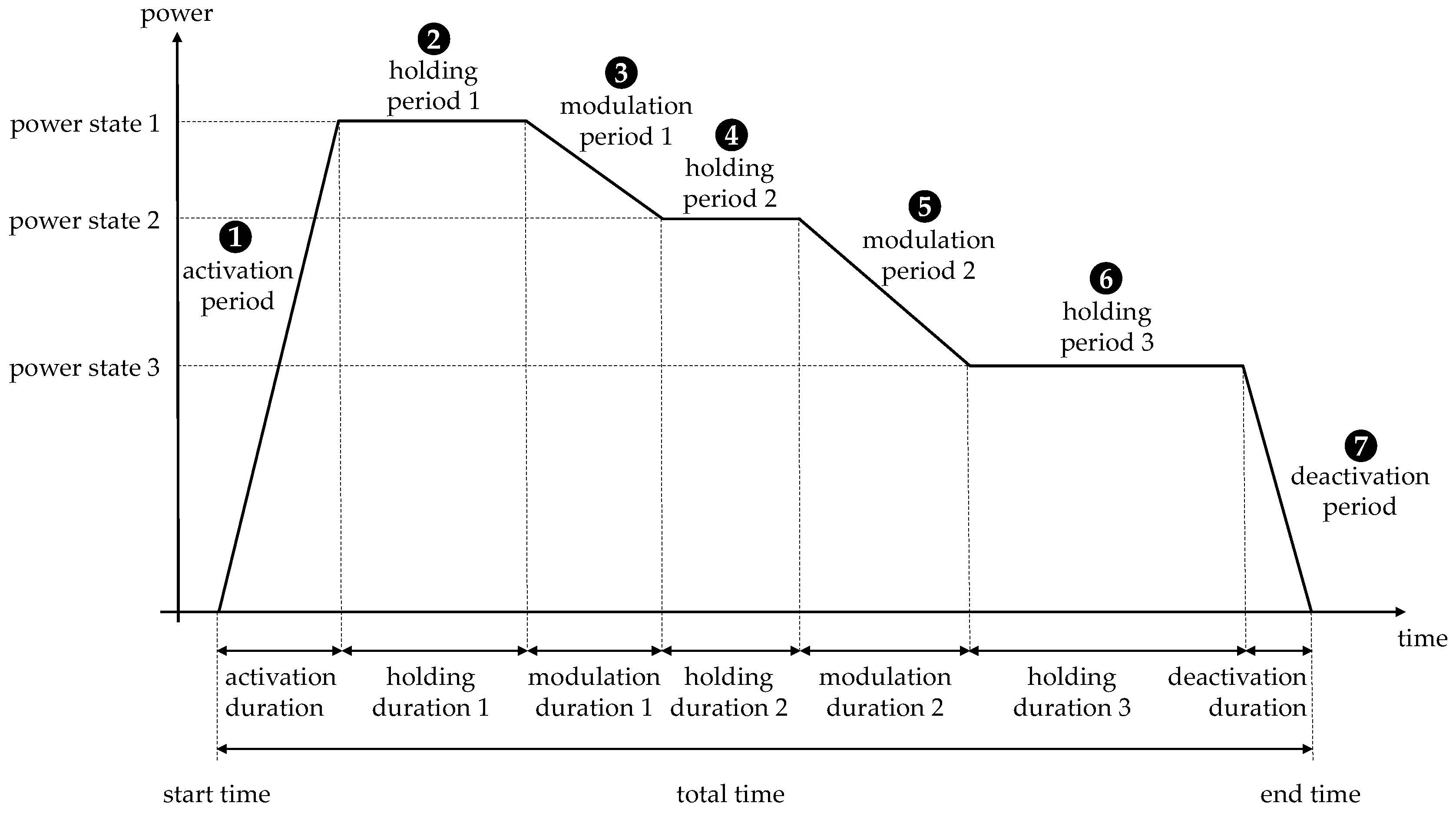
which can be described by means of periods of constant increase or decrease in load (“modulation periods”), and periods of constant load (“holding periods”). Note that although mathematically periods of constant load are a special case of the former with the rate of change (slope) being zero, we distinguish these periods in order to foster intuition and to account for the different characteristics of the physical processes. One can regard our approximation as a specific linearization of load curves. However, it is important to highlight that we do not linearize a fixed function, but rather a collection of functions, and thus preserve the degrees of freedom.
Figure 3 illustrates an exemplary flexible load measure, i.e., one special load curve in the family which is meant to be parametrized by the key figures of the corresponding flexible load. In
Figure 3, the different phases and their respective durations are depicted.
Apart from power consumption depending on time, a flexible load also exhibits some other relevant characteristics, such as integration in an IT-system or costs, which have to be included in our data model. With this preliminary work, we are now prepared to discuss all the key figures of the subcategory flexible load.
3.2.1. Flexible Load ID
A company can have a large number of devices which exhibit flexibility. Within a company, production is usually managed and controlled via an IT system, for example an ERP system. To be able to easily manage them, a flexible load thus requires a
flexible load ID. The available systems must also consider the
flexible load IDs. The key figure
flexible load ID is used to uniquely identify a flexible load and hence to address the corresponding device in case it is used. As will become clear in
Section 3.3.1, it is explicitly possible that multiple flexible loads with multiple
flexible load IDs refer to the same device. This key figure is important when execution of a (specific) flexibility measure must be ordered by the IT system of a company.
3.2.2. Reaction Duration
In case the execution of a flexible load measure is ordered, it is highly relevant how long it takes from giving the command to activate until a change in power really starts. For this reason, it is necessary to add the key figure reaction duration to our model. In an automated system, this is comparable to the latency time that occurs during the transmission of signals. For processes that still require a lot of manual effort, the reaction duration can also refer to other kinds of delay. For example, an employee might need some time in advance in order to prepare a machine accordingly. Therefore, the reaction time can be interpreted as the duration between pulling the trigger and the start time of the flexible load measure. The reaction duration is of high relevance especially in time-critical applications. For example, in the case of control power, flexibility must be provided within a short period of time. Of course, we make the assumption that a company can determine the reaction duration. This is particularly challenging when the response time is not just given by the latency time of an IT system. The reaction duration in our data model has the unit seconds and is given by a real number which by causality is non-negative.
3.2.3. Validity
Flexible loads are usually only available within certain time windows. The reason is that, for companies, compliance with delivery obligations naturally has a higher priority than the utilization of flexibility. Hence, restrictions associated with time of use can depend, for example, on the production plan, since this determines when machines operate and could be switched off. Another reason is that machines may have to be maintained and operated during shift times and are therefore not always available. Moreover, for many electricity-intensive companies, technical restrictions or grid fees pose a central boundary condition regarding time periods of increased electricity consumption. Therefore, the key figure
validity is an essential part of the data model and serves to consider restrictions with respect to availability over time. We use it to define when flexibilities may be used. Consequently,
validity is a subset of the planning horizon. As opposed to other key figures, we assume that the
validity is fixed and does not depend on any other key figure. As for the planning horizon, our unit here is seconds since 1 January 1970. Recalling the example of shift times, we cannot expect that it is usually an interval. In SynErgie, we have investigated a wide range of flexibilities, some of which have quite special temporal characteristics. For example, it is common for some companies to start flexible processes within a certain time window. By contrast, other processes have to be completed at a certain point in time. Another observation was the necessity to define a time window in which the whole execution of a flexible load must be completed. Therefore, we need to define the
validity with respect to a certain reference. Based on our observations, the following three references are necessary: “start”, “total”, and “end”. The reference “start” indicates that the start time of a flexible load measure must lie within the
validity. Similarly, the end of a flexible load measure must lie within the defined interval for the reference “end”. The reference “total” specifies that the entire load profile of a flexible load measure must lie in the interval specified by the key figure
validity. This distinction is particularly relevant for flexible loads with many degrees of freedom. For these, start time, end time, and total time can usually not be converted into each other at the level of a flexible load. As already mentioned, these three references were sufficient in order to encompass all the flexible loads which we encountered in SynErgie. However, one could think of special cases which can not be expressed by any of the three proposed references. For example, imagine that the first half of a process must be completed within the
validity since it must be supervised by an employee. However, note that, by splitting this example into two separate flexible loads and defining suitable dependencies (see
Section 3.3), one could even model such cases with our data model.
3.2.4. Power States
As already discussed, industry processes can usually operate at different levels with regard to power consumption. That is why we introduce the key figure
power states. It defines the admissible power levels of the plateaus, i.e., during holding periods (see
Figure 3. Depending on the choice of perspective, both the absolute power values and the deviation from the scheduled load can be defined as
power states. With
power states, we describe situations in which devices have a constant power consumption. Of course, these can also be very short periods of time.
Power states for subsequent holding periods may be different, in fact, this is the case for all variables which need to be specified repeatedly. For the key figure
power states, both continuous and discrete subsets of the real numbers are possible as basic sets. Continuous
power states occur, for example, in cooling units. Here, the power consumption can be set almost arbitrarily within a specific interval. On the other hand, there are processes, e.g., electrolysis, in which only discrete
power states are permitted. The unit for
power states are chosen to be kW. A positive resp. negative sign represents an increase resp. a decrease in electricity consumption.
In reality, the actual electricity consumption is rarely constant. However, in the energy industry, the time interval of 15 min is established as the shortest observation period. On power markets, for example, the products with the shortest duration are 15-min products. This implies that our assumption of constant consumption in certain segments is practicably as good as an exact modelling. In this case, it is important to keep in mind that the key figure power state does not precisely represent the actual physical state.
3.2.5. Holding Durations
As we already mentioned above, the key figure power states is related to temporarily constant states. Machines often need electricity for a certain period of time, e.g., to manufacture a product. The durations of power states are specified by the key figure holding durations. The holding duration specifies the range in which the chosen power state may be held. As a unit, we choose the SI base unit seconds. Analogous to the power states, we adopt the simplified view that the actual duration is known exactly in advance. Of course, in reality, it can happen that processes are completed earlier or later than planned.
3.2.6. Usage Number
In practice, we observed many flexible loads which admit multiple runs within their validity. For instance, when manufacturing a product, a production step must be repeated. To avoid the need for defining several identical flexible loads which are mutually exclusive during their time of use, the data model contains the key figure usage number. It describes the number of permitted activations (usages) of a flexible load within its validity. The usage number is given by a subset of the natural numbers (including zero). We want to emphasize that it is not necessary to select identical flexible load measures in repeated usages. For example, if was selected for the first usage, a different can be selected for the second use. However, by definition, the corresponding ranges can depend on the usage number*. For instance, in a thermal process, it is likely that multiple usages will require either a smaller power state or a shorter holding duration. If a company is aware of these relations, the power states in this example could be a function of the usage number.
3.2.7. Modulation Number
So far, we have had the picture in mind that flexibilities have exactly one holding period, after which the load profile returns to the zero state. However, there are many processes that can adapt their
power state during one usage several times (see
Figure 3). A usage refers to the sequence of:
Power state is equal to zero, followed by some changes in power consumption, and ends again with a
power state of zero. As an example, one can think of heating processes, which modulate their
power states from time to time. In addition to industrial processes, power plants can also be considered: As soon as these are operated, the
power state changes several times before the power plant is switched off again. This leads to the key figure
modulation number. It states the number of modulations (changes of the
power state) which may take place during one usage of the process. Activation and deactivation are regarded as special cases of a modulation, since the restrictions posed on the initial and final power change are often different from the ones posed on modulations in between. The
modulation number is given by a subset of the natural numbers.
3.2.8. Activation Gradient, Modulation Gradients, and Deactivation Gradient
With regard to the activation, modulation, and deactivation phases, the intensity or speed of the power change is a relevant parameter. It can, for example, be restricted due to constraints when heating material. Moreover, many devices cannot be switched off at arbitrary speed. We introduce the key figures activation gradient, modulation gradients, and deactivation gradient. The corresponding durations can easily be calculated from the respective gradient and the difference in neighbouring power states to be reached. Respecting the units for power states and holding durations, we define the unit to be . All gradients are given by subsets of the extended real numbers, i.e., we also allow plus and minus infinity as legitimate gradients. This makes sense with the convention , since in an optimization the only relevant quantities are energy consumption and time which are both indirectly proportional to the gradients. The activation gradient resp. deactivation gradient specifies which slopes the load curve can exhibit during the activation resp. deactivation phase. The key figure modulation gradients is the analog for modulation phases. The activation and deactivation gradients are required in addition to the modulation gradient since the speed of activation and deactivation often differ from a modulation. If a machine has already been warmed up, it can usually change its output more quickly. Thus, it is likely that the modulation gradients may depend on previous power states and the holding durations. The deactivation gradient is the analog of the activation gradient for the deactivation phase. We adopt the convention that a positive gradient for activation, modulation, and deactivation always means that power consumption increases with time. As for power states and holding durations, we simplify the real world by linearization here.
3.2.9. Regeneration Duration
Often, one has to wait some time after a flexible load measure has been activated until another flexible load measure from the same flexible load may be activated again. This might be necessary for maintenance, chilling, or warming of the corresponding machine or product before reuse. In processes that are not yet highly automated, employees often need to remove the finished product from a machine and load the raw materials into the machine again. This characteristic must be taken into account especially for flexible loads with potentially multiple usages. Therefore, we include the key figure regeneration duration into the flexible load data model which specifies the time span in which, after completion of a flexible load measure, the flexible load must not be activated again. In other words, the regeneration duration refers to the minimum waiting time in seconds after the end of a flexible load measure. A regeneration duration of 0 seconds means that right after a flexible load measure has ended, another flexible load measure from the same flexible load may be activated. In practice, this key figure often depends on the characteristics of other key figures. If, for example, the regeneration duration is caused by a cooling process, the regeneration duration can probably depend on the previously attained power states and holding durations. This also goes along with the limitation that these relations must be exactly known in advance in order to be able to model the regeneration duration exactly.
3.2.10. Costs
The flexible operation of machines usually causes additional costs. They might stem from higher expenses, e.g., due to higher wear and tear of machines in atypical operation. It is also conceivable that increased personnel hours and associated expenses such as handling and maintenance must be accounted for here. In addition, for some machines, manufacturers give a warranty covering a certain number of power changes. As soon as this is exceeded due to frequent usage of a flexible load, the warranty for the corresponding machine expires. This circumstance must also be taken into account.
For this reason, the key figure costs is also part of the data model. The unit of this key figure is the chosen currency, in our case, Euro. We explicitly do not include electricity costs in this key figure. The reason is that these depend on company-extrinsic parameters such as (expected) electricity price and are not necessarily known in advance. However, from integrating the product where denotes the (expected) electricity price at time , one can easily calculate the (expected) electricity costs. The key figure costs is likely to have dependencies on other key figures. For example, high values for power states or gradients can influence the degradation of the infrastructure and thus the associated costs. With regard to costs, the limitation is that companies must know the relations exactly. Otherwise, if the exact costs are unknown, one can define a threshold value to consider an increased risk of wear and tear. In the end, the costs decide whether a flexibility is used or not. Therefore, they must be modelled as accurately as possible. However, since most industrial machines are designed for continuous operation, the costs incurred are often not known.
3.2.11. Summary: Flexible Loads
Table 1 provides an overview of all presented key figures which we use to describe flexible loads. With regard to the convention of plural or singular key figures, we have defined the following: key figures that can have more than one value during one usage are denoted in the plural, the remaining key figures—apart from costs—are in the singular.
3.3. Dependencies
As already mentioned in
Section 3.1, we observed that there are often logical constraints among different flexible loads. A dependency describes the impact of an activation of a measure corresponding to a certain flexible load on another measure from a different flexible load. We observed that two logical types, namely implication and exclusion among pairs of flexible loads, are sufficient in order to describe those logical constraints. However, extension to more flexible loads as inputs would be straightforward, but would also make the data model more complicated. In the following, we describe the key figures which specify a dependency.
3.3.1. Trigger Flexible Load, Target Flexible Load, and Logical Type
A dependency always refers to a pair of flexible loads. Therefore, we introduce the two key figures trigger flexible load and target flexible load. This means that usage of any of the flexible load measures from the trigger flexible load poses some constraint on the usage of the target flexible load.
In addition, it is necessary to describe the dependency type. By an “implies”-dependency, we mean that, for every usage of a flexible load measure from the trigger flexible load, some uniquely associated flexible load measure from the target flexible load must be activated. In particular, the usage number* of the trigger flexible load in the planning horizon cannot be larger than the usage number* of the target flexible load. We realized the need for the “implies”-dependency for the following situations: In several production processes, a certain order of steps needs to be fulfilled. As another example, if the output is reduced at a certain point in time, the production that has to be renounced must be recovered at a later stage by increasing the output.
On the other hand, an “excludes”-dependency states that the usage of some flexible load measure from the trigger flexible load forbids usage of any of the flexible load measures in the target flexible load. The “excludes”-dependency is necessary, for example, in order to avoid consumption peaks, which are relevant for network charges. Moreover, it can be used to model a device which is involved in very different processes such that the flexibility associated with this device can not be described by only using a single flexible load.
Note that, by combining two dependencies with suitable trigger flexible loads, target flexible loads, and logical types, one can also model further logical interrelations such as “if and only if” and “exclusive or”.
3.3.2. Temporal Type and Applicability Duration
In order to respect the temporal characteristics of the dependencies that we observed in SynErgie, we also introduce the key figures: Temporal type and applicability duration. The reason is that, for both “implies”- and “excludes”-dependencies, one must be able to specify the period for which these dependencies are valid. The key figure applicability duration represents this property. It is given by a subset of the real numbers (typically an interval) and has the unit seconds. In the case of an “implies”-dependency, the applicability duration states that within the specified period the target flexible load must be activated. Similarly, for an “excludes”-dependency, the applicability duration indicates that the target flexible load must not be used during this time.
The applicability duration can have different reference points. Thus, analogous to our approach for the key figure validity, we need to add a time reference. Therefore, we introduce the key figure temporal type. Since the reference must be applied to both the trigger flexible load and the target flexible load, the temporal type is given by a tuple, consisting of combinations of “start”, “total”, or “end” in both components. The first component refers to the temporal reference for the trigger flexible load, the second to the target flexible load. Combining applicability duration and temporal type, a flexible load measure from the trigger flexible load yields an interval in which the flexible load measure of the target flexible load must or must not lie.
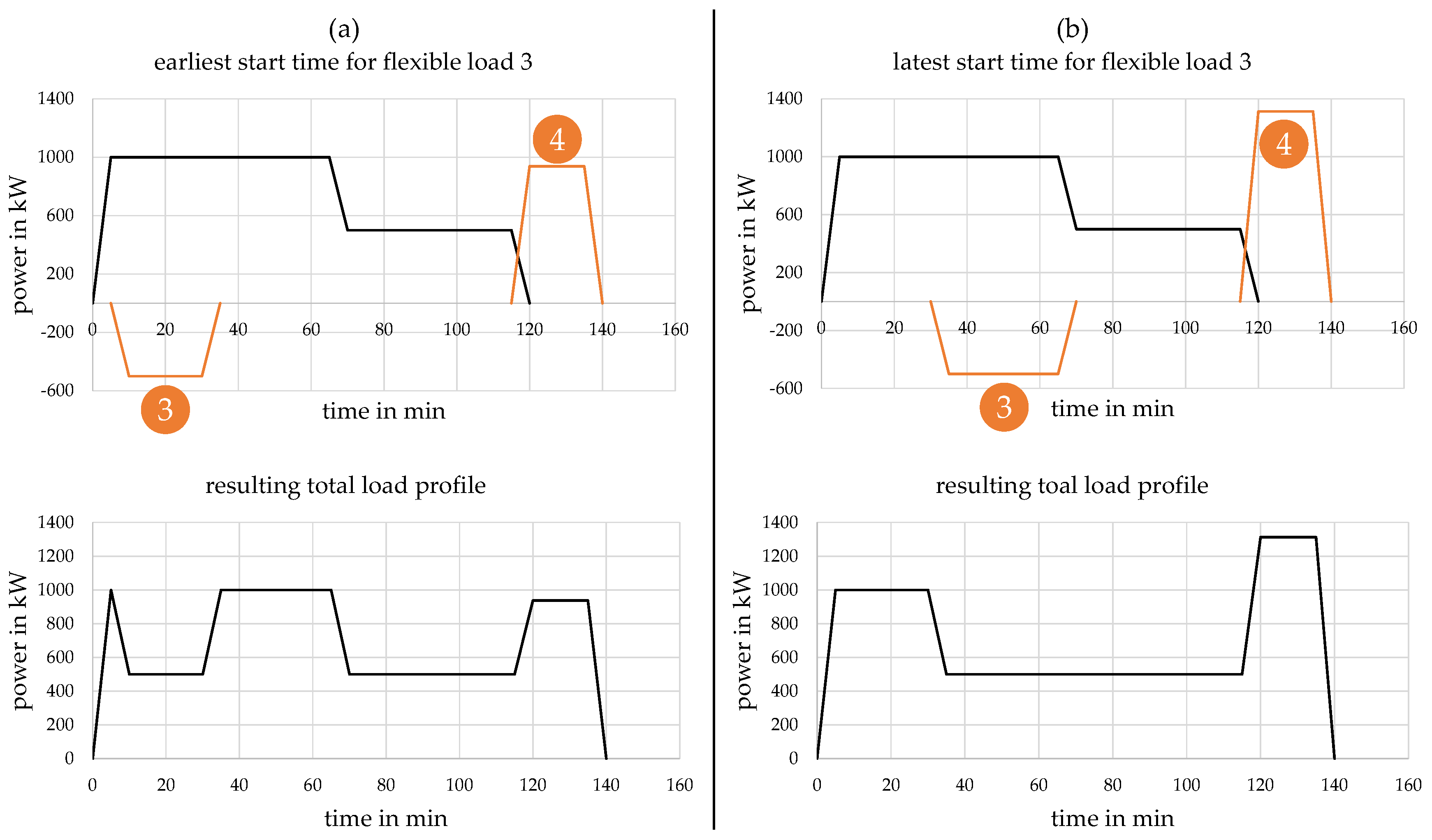
Figure 4 visualizes some possible combinations of these two key figures. For a specified
trigger flexible load A, the figure illustrates the accessible times for the usage of the
target flexible load B. The holding duration of flexible load A is fixed and given as depicted, and the
applicability duration is given by
. The orange bars denote the part of the planning horizon in which—once a measure in flexible load A has been determined and hence in particular the temporal component is specified—a measure from flexible load B may be activated. For simplification, we assume that the temporal component for flexible load B is also fixed. Then, the part of the total usage duration of flexible load B which is coloured in orange must lie within the orange bar.
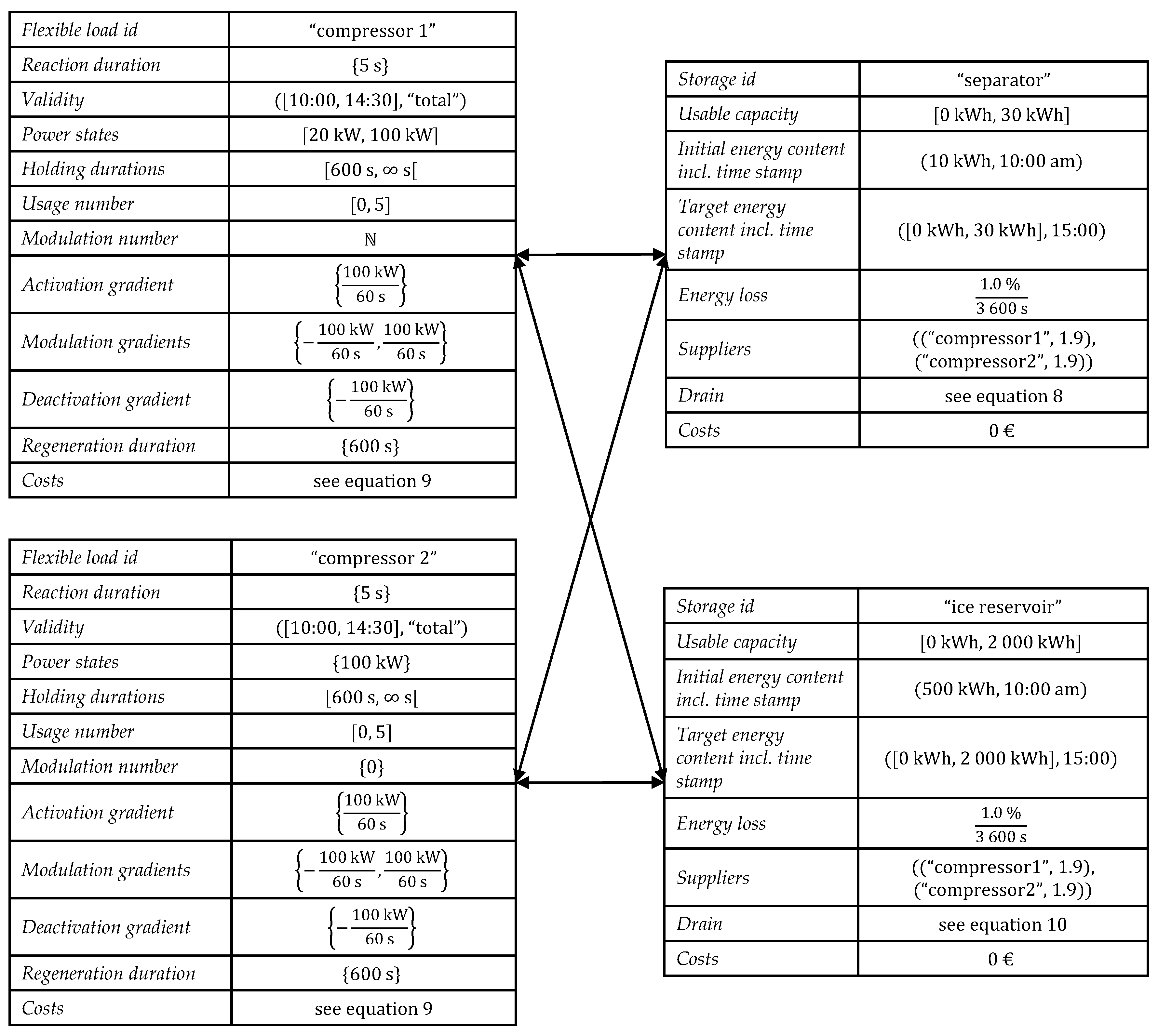
The following practical examples further illustrate the possibilities of combining dependencies with different applicability duration and temporal type. The trigger flexible load is called “C” and the target flexible load is called “D”. Firstly, due to process interdependencies, C and D should not be active at the same time. For this example, logical type has the value “excludes”, the applicability duration is and the temporal type is {“total”, “total”}. Secondly, as the material has to be replaced in machines after completion of process C, further processing D can be carried out at the earliest 20 s after completion of C. At the same time, D must be completed two minutes after C at the latest. Therefore, two additional dependencies must be defined: One with logical type “excludes”, applicability duration , and temporal type{“end”, “start”} ensures that D does not start earlier than 20 s after C. The second dependency with logical type “implies”, applicability duration , and temporal type{“end”, “end”} ensures that D ends two minutes after C at the latest.
Finally, we want to highlight that—strictly speaking—the regeneration duration which we defined for flexible loads is a special case of a dependency. In this case, trigger and target flexible load are identical, and logical type, temporal type, and applicability duration are given by: “excludes”, (“end”, “start”), [0, regeneration duration*]. However, the regeneration duration can be regarded as an intrinsic property of a flexible load, and only requires the specification of one parameter, which led us to define it as a separate key figure.
3.3.3. Applicability Conditions
In the case of dependencies between two flexible load measures, in SynErgie we have often observed that there are additional conditions which need to be fulfilled. These can be defined in the key figure applicability conditions. Every condition is described by an equation which refers to key figures of the two involved flexible loads. The first resp. second component of the tuple which represents the equation are regarded as left resp. right-hand side of the equation. The applicability conditions are regarded to be satisfied if for every , both components of the component of applicability conditions have the same value. A constraint posed by a dependency which exhibits applicability conditions are not satisfied, the dependency is regarded is only then regarded as fulfilled if the applicability conditions are met. In other words, an activation of the trigger flexible load implies an associated activation of the target flexible load—respecting the constraints given by the other key figures—in a configuration (measure) such that the applicability conditions are satisfied.
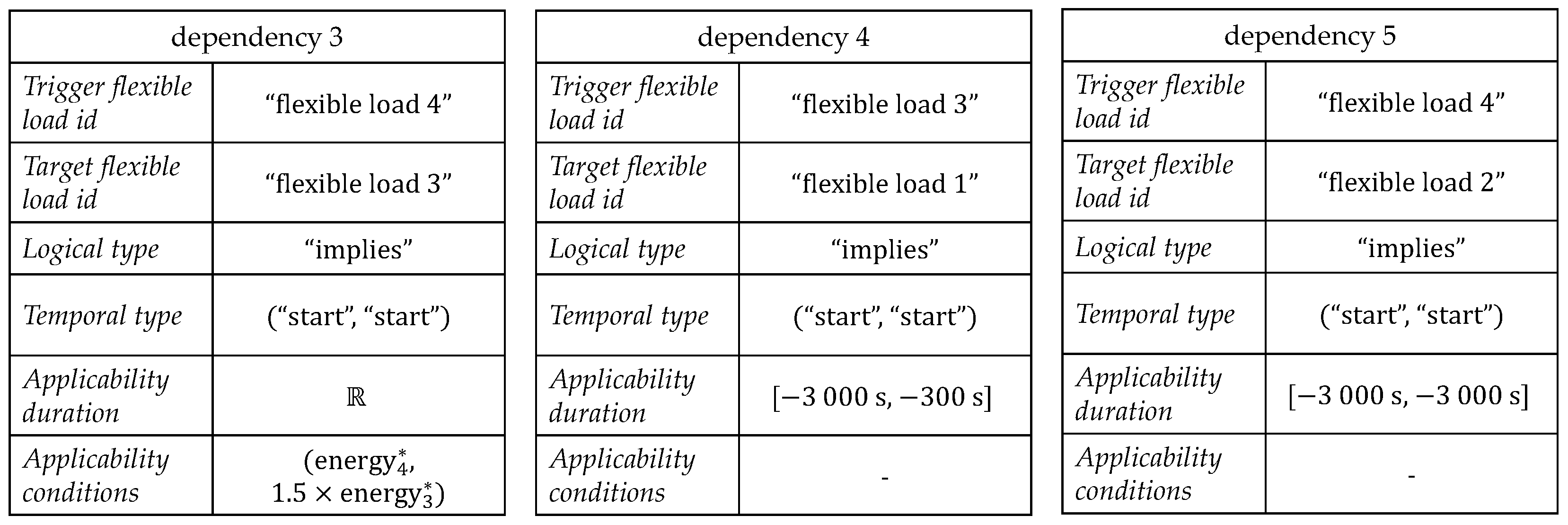
As an illustrative example, imagine a process in which flexible load A describes the opportunity to reduce power consumption at a given point in time. By means of flexible load B, the energy can then be recovered. For instance, due to losses in efficiency, flexible load B must make up 1.5 times the energy of flexible load A. Therefore, the
applicability condition is given by the tuple
. The pre-factor of 1.5 means that flexible load B must consume 50% more power due to losses, which enforces the following equation:
Flexible load A has only one
power state {−500 kW}, but a variable
holding duration with permitted range
. The
modulation number is zero in this case. Flexible load B, on the other hand, has the fixed
holding duration {900 s} and a variable
power state , 10,000 kW]). The constraint in Equation (
1) specifies that the
power state of flexible load B must be chosen according to the configuration of flexible load A. The relevant
power state can be calculated as follows. First, it is necessary to calculate the electricity consumption of flexible load A. For a given
power state, the power consumption of flexible load A which corresponds to the area of the rectangle (the gradients are assumed to be infinite here) is as follows:
The power consumption of flexible load B is calculated as follows, whereby the
holding duration is given:
By merging Equations (
2) and (
3), the additional constraint—which ensures that flexible load 2 catches up 1.5 more electricity than flexible load 1—can now be determined:
This example illustrates which additional restrictions can be modelled by the key figure applicability conditions.
3.3.4. Summary: Dependencies
Table 2 summarizes all key figures of the dependency subcategory including type, unit, and description.
3.4. Storages
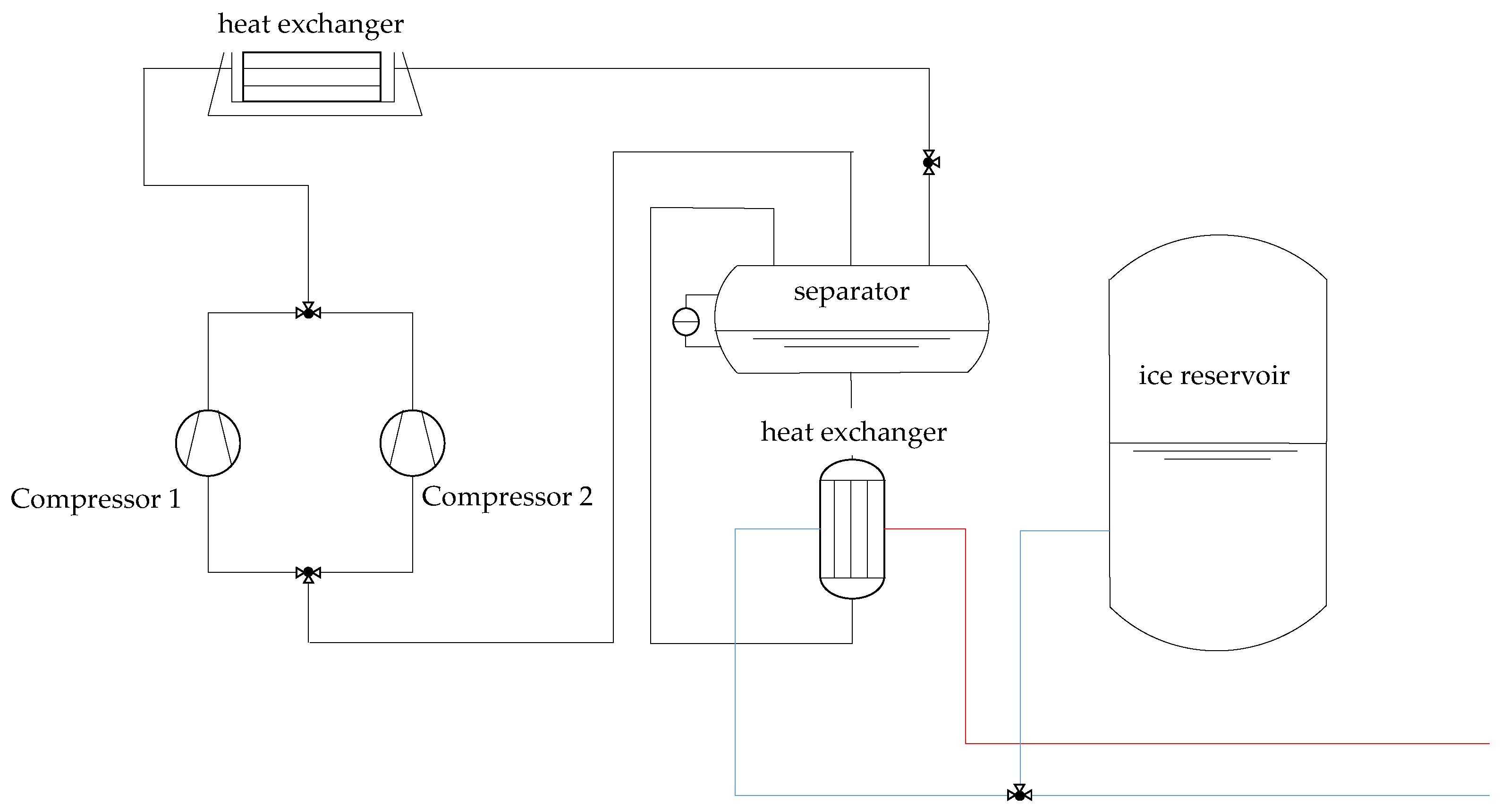
Energy storages are classically understood to be electrical storage devices such as batteries that have a certain storage capacity. Apart from these conventional storage systems, industrial processes often have storage potentials that can be described with similar key figures. They usually appear in form of stock for batch processes, thermal inertias, or reserves of intermediate products such as chemicals. The form of energy in a storage device is not limited to electrical energy. All forms of effective energy, e.g., heat, cold, and compressed air, whose provision is connected to a flexible load and any product whose manufacturing (or disposal) requires electrical energy can theoretically be stored. In the following, we present the key figures which are necessary for describing storage.
3.4.1. Storage ID
Just as it is important for flexible loads to have a clear designation (see
Section 3.2.1), it is also for storage systems in industrial processes. Therefore, the key figure
storage id is implemented. This key figure is an identifier for storage in the company’s IT system and assigns a unique name to the respective storage system. This is particularly important if a storage is connected to several flexible loads or if one flexible load can supply different storages (see
Figure 1). For example, an intermediate product or raw material warehouse can serve different devices.
3.4.2. Usable Capacity
The indication of capacity is indispensable for the characterization of a storage facility as it limits the quantity of the good resp. energy to be stored. Therefore, the key figure
usable capacity is part of the data model. However, in the context of energy flexibilization, it is often not the maximum energy content of a storage facility that is relevant, but the proportion available for flexibilization. One example are thermal storages. While, from a physical point of view, one would have to refer to the ambient temperature or the temperature zero point when calculating the energy content, the capacity of interest in the context of energy flexibility is usually limited by the minimum and maximum process temperatures allowed. Batteries are another example. With a nominal storage capacity of 30 kWh, the
usable capacity (which in literature is sometimes also-called useful capacity in the context of batteries) might be restricted, for example to extend the lifetime of the battery storage, as this is depending on the depth of charge and discharge cycles [
29]. Although not all storage systems directly refer to energy quantities, a representation in the form of energy quantities is reasonable in order to compare different types of storages and suppliers (see
Section 3.4.6). For example, the energy content of a thermal storage can be compared with that of a compressed air system. The
usable capacity is specified as an interval in kWh whose lower bound may never be undershot and whose upper bound may never be exceeded by the energy content of the storage.
3.4.3. Initial Energy Content
It is important to specify the energy content in the storage—the initial energy content—at a specific time stamp. For example, a fully charged storage facility cannot be used directly to provide a load increase. If the storage facility is operated over several charging cycles during long planning periods, the initial energy content usually has less influence on the result than if only one charging cycle is considered. This key figure is specified in kWh and the corresponding time stamp in seconds.
3.4.4. Target Energy Content
In some cases, a specific energy level must be reached in the storage at a certain point in time. Examples for this are batteries of intralogistics vehicles, which should be fully charged at the beginning of a shift. Another example are product warehouses, which must be full as soon as the delivery date is due. These circumstances can be defined in the key figure target energy content with a corresponding time stamp. It is not necessary and expedient to specify an exact target energy content in all cases. Often it is sufficient to know which upper and lower limits must not be exceeded for the energy content of the storage (usable capacity). In general, the target energy content is defined as a subset of the usable capacity. Its unit is kWh and the time stamp is given in seconds.
3.4.5. Energy Loss
Many storage types are characterized by time-dependent losses of the medium to be stored. For example, the temperature of thermal storage tanks adjusts to the ambient temperature over time, which means that the exergy to be stored gets lost. Compressed air reservoirs also lose their pressure level due to leakages of the storage system. In order to take these unavoidable losses into account, the key figure energy loss is necessary. It is defined as the share of the current energy content which gets lost every time period in , in the planning horizon.
3.4.6. Suppliers
The linking between flexible loads plays a fundamental role in modeling systems with energy storages. For example, a product warehouse can be filled by different production systems or a compressed air reservoir by different compressors. Depending on the suppliers or the storage facility, a specific efficiency is achieved with which the energy storage facility is filled. Thus, two machines which fill the same warehouse can produce the same product with different efficiency. If the product is now considered with an energy equivalent, this results in a different conversion efficiency for the two machines. The same applies to two compressors filling a compressed air reservoir with different degrees of efficiency. Not only is the efficiency of the energy converter relevant, but also the storage type. For example, a 12 bar compressed air storage is charged with a significantly lower degree of efficiency than a 6 bar storage. For this reason, the linking between a flexible load and storage is modelled via an ID of the supplier with an associated efficiency description. The degree of efficiency can depend on all key figures of the supplier.
3.4.7. Drain
In many cases, unchangeable loads must be served during production. In contrast to suppliers, a drain does not provide any flexibility and therefore only represents a fixed deterministic demand. In the data model, the drain is therefore given by a function which assigns to every time in the planning horizon the power in kW which is flowing off.
3.4.8. Costs
Costs can occur not only during the conversion of energy, i.e., with regard to flexible loads, but also at the time of storage. Certain charging strategies can lead to increased storage wear, which in turn increases costs in the long term. For example, lithium ion batteries do not withstand high power gradients or deep discharges. We assume that the costs of storage only depend on its (time-dependent) energy content. It is important to note that this figure only includes storage-related costs. Costs arising from the flexible operation of the suppliers must not be taken into account here since they are already included in the data model for flexible loads.
3.4.9. Summary: Storages
The derived key figures enable the modeling of various storages, e.g., product or electricity storages in industry. Note that the key figures of storage are in general not interrelated with other key figures of flexible loads, dependencies, and storages. However, there are two important exceptions: First, the conversion efficiency associated with a
supplier, i.e., a flexible load, may depend on key figures of precisely this flexible load. Second, the
costs induced by storage may only depend on the (time-dependent) energy content of the respective storage. The key figures contained in the data model and the associated types, units, and descriptions are summarized in
Table 3.
4. Data Model for Flexible Load Measures
We already mentioned in
Section 3.1 that we need an additional data model to describe flexibility measures. Ultimately, the aim of the data model for a flexible load measure is to specify a load curve in concrete terms. On the other hand, since for an optimization we need to assign specific costs to flexibility measures and hence flexible load measures, it is necessary to be able to compute the costs from the realized key figures. This would be complicated if the data model for a flexible load measure is very different from the data model for a flexible load, e.g., by just defining the resulting load curve as a function: in this case, it would be tedious to recover key figures like
gradients* or
holding durations*. However, the costs for flexible loads are in general precisely functions of these key figures.
What we want to emphasize here is that, although the way from a generic data model for flexibilities, which clearly is the focus of this article, to a generic data model for flexibility measures is quite straightforward, it is not completely obvious and potentially leaves ambiguities. Hence, we also provide a standardized model for flexibility measures.
The data model presented in
Section 3 is the basis for the description of flexibility, i.e., spaces with degrees of freedom. One might expect that a single element in a flexibility can be specified by a choice for every key figure in every flexible load, dependency, and storage contained in the flexibility. For such instances, which according to
Section 3.1 we call flexibility measures, constraints no longer have to be taken into account. Thus, all key figures for dependencies and storages can be neglected.
Hence, the next guess would be that only for the contained flexible loads, choices for the key figures have to be made. However, describing the potentially repeated usages of a flexible load in a single object would be confusing. The announced flexible load measure therefore is only meant to describe a single usage of a flexible load. In other words, for every flexible load contained in a flexibility, a corresponding flexibility measure contains usage number* associated flexible load measures. In order to distinguish key figures which refer to a choice (*) of a value in the data model for flexible loads and key figures for flexible load measures, we denote the key figures which do not occur in the final data model for flexible load measures in roman. Since the latter are not of intrinsic interest but only relevant in a supportive way, we do not provide details of the associated object any further.
In order to develop a data model for flexibility measures, it therefore suffices to specify a data model for flexible load measures. The first idea is to do this based on the key figures of a flexible load, ignoring the key figure
usage number since this information is already contained in the number of flexible load measures in a flexibility measure. Moreover, we can eliminate the key figure
regeneration duration, since, as we explained at the end of
Section 3.3.2, this is just a further dependency. Additionally, since the usage time for a flexible load measure is fixed, we can simplify the key figure
validity to
start time*, and a reference is not needed any more.
Some key figures of a flexible load have to be chosen multiple times in order to fully specify a flexible load measure. These key figures are:
power states,
holding durations, and
modulation gradients. Consequently, the related key figures for flexible load measures which correspond to these three key figures of flexible loads are given by vectors. Moreover, we merge all gradients to one combined key figure, since we no longer have to distinguish activation and deactivation from modulations (see
Section 3.2.7). The length of these vectors, in turn, depends on the
modulation number*.
Summarizing, our data model for flexible load measures enables retaining all storage key figures for the measures in order to be able to check the status of the storage or the fulfillment of a dependency, for example. As already mentioned, the length of some vectors depends on the number of modulations. For brevity, we define the exponent
m as follows:
The key figures contained in the data model for flexible load measures are summarized in
Table 4.
6. Discussion
As described in
Section 3 and
Section 5, the presented data model can be used for describing a wide variety of flexibilities.
Finally, we want to challenge our data model with the checklist developed by Barth et al. [
24]. As already described in
Section 1, in their paper, the authors define flexibility features which represent different attributes of flexibility.
Table 5 lists the flexibility properties of Barth et al. [
24] and their corresponding descriptions as well as the way these features are covered by our data model.
Our detailed analysis demonstrates that all features defined by Barth et al. [
24] can be covered with the presented data model. In addition, certain types of flexibility, such as storages, can be modelled more easily and precisely, since they do not have to be mapped via discrete jobs. The reason for this is the modular structure of our data model. Furthermore, it is possible to describe instances of the so-called job shop scheduling problem (example 1 in
Section 5) as well as the conventional unit commitment problem like example 2. This allows a large part of the industrial flexibility to be mapped sufficiently. The industry partners in SynErgie all consider our modeling approach suitable. Therefore, we are convinced that our results are of substantial relevance. It thus fulfills its purpose of the standardized description of flexibility potentials for further use in various applications. Moreover, additional characteristics like the reaction duration or more complex behavior like warm start or cold start of machines can be described via the dependency of different flexible loads. In order to verify the applicability of the data model in industry, numerous rounds of discussions were held with industry representatives and scientists. A wide variety of applications were considered—for example, graphitization, heat pumps, refrigerated warehouses, or paper production.
In the course of the project, we also described flexibilities in close collaboration with companies from the mentioned industries in our generic data model. For this purpose, we used Java to implement the data model and used JSON-files to represent the corresponding flexibilities. With regard to the applicability of our data model, one must distinguish two perspectives: The first question which arises is whether the data model can represent the flexibilities of a company. Secondly, it is also vital that the corresponding users are able to fill the data model. Our discussion suggests that it is indeed possible to represent the relevant flexibilities in our data model. On the other hand, we have observed that, for companies, filling out the data model for the first time is not always intuitive. However, the modularity of the data model also allowed to describe complex processes and provided a guideline to capture an understanding of the flexibility. Since the key figures stay the same for every flexibility, with repeated usage of the data model, it becomes increasingly familiar and comfortable to use.
In our validation, we have focused on the industrial sector. As already mentioned, the characteristics of our data model and our generic approach allow for transferring the model also to other types of power-related flexibility such as plug-in electric vehicles. Note that, in our presented data model, we can represent a plug-in electric vehicles by a flexible load (the plug) and storage (the battery). Costs incurred by charging and discharging (cycling degradation) the electric car can be captured in the key figure
costs of the subcategory flexible loads [
29]. Moreover, costs arising from the use of the battery (depth of discharge) can be modelled in the key figure
costs of the subcategory storages [
29]. By specifying suitable dependencies in our data model, one can even include additional characteristics related to charging infrastructure such as limited numbers of charging stations or grid constraints in certain areas. A detailed analysis of the applicability for all the above-mentioned sectors, however, must still be conducted in future research. It is important to keep in mind that the flexibility provided by electric vehicles also exhibits a stochastic component, namely whether it is in use or connected to the power system? However, the stochastic aspect needs to be part of the load planning and systemic considerations. The data model is meant to describe the actual flexibility, i.e., once it is known that the electric vehicle is plugged in and the earliest departure time (which then defines the
validity) and the
initial energy content are known, the corresponding flexibility can be offered in our data model.
7. Conclusions
The focus of this article was the description of generic, power-related flexibilities. The modular structure of our data model allows us to model various flexibilities. We modeled flexibilities as subsets of at least one flexible load. The corresponding constraints were described by the subcategories dependencies and storages. The modular structure enables an efficient description of both simple and complex processes. The data model thus forms the basis for describing flexibility. The two examples which we analyzed in
Section 5 illustrate our data model and stand for a multitude of real-world industrial applications which we investigated in the Kopernikus-project SynErgie (see
Section 2). As mentioned in the introduction, the information layer of the Smart Grid Architecture Model is intended to ensure standardized communication. The data model presented in this article enables a standardized description of flexibility in the Smart Grid Architecture Model [
17]. Thus, the data model is also relevant for the business layer in order to market the flexibility.
Based on the description of flexibility in the form of the data model, the use of flexibility for different objectives can be investigated. For example, the uncertainties in the feed-in of renewable energy sources can be addressed. This can increase the share of renewable electricity. In the same way, knowledge about flexibility can be used for efficient network operation and can help to minimize network expansion [
7,
30]. Furthermore, the data model enables flexibility providers to optimize the use of flexibility with regard to financial aspects [
6]. Therefore, we are convinced that the presented data model provides an essential basis for the automated use of flexibility. In this way, more flexibility can be exploited in the future to close the emerging flexibility gap [
5].
It is relevant for future research to develop a suitable optimization model based on the presented data model. On this basis, the use of flexibility, here we focused on the demand side, can then be optimized. In order to take an integrated view of the electricity system, the feed-in characteristics from renewable energies must be examined in more detail in future research. Accordingly, future research must also deal with a generation model for fluctuating renewable energies.

 ,
, 


