Multi-Objective Hybrid Optimization Algorithm Using a Comprehensive Learning Strategy for Automatic Train Operation

Abstract

Aiming at the problem of easy-to-fall-into local convergence for automatic train operation (ATO) velocity ideal trajectory profile optimization algorithms, an improved multi-objective hybrid optimization algorithm using a comprehensive learning strategy (ICLHOA) is proposed. Firstly, an improved particle swarm optimization algorithm which adopts multiple particle optimization models is proposed, to avoid the destruction of population diversity caused by single optimization model. Secondly, to avoid the problem of random and blind searching in iterative computation process, the chaotic mapping and the reverse learning mechanism are introduced into the improved whale optimization algorithm. Thirdly, the improved archive mechanism is used to store the non-dominated solutions in the optimization process, and fusion distance is used to maintain the diversity of elite set. Fourthly, a dual-population evolutionary mechanism using archive as an information communication medium is designed to enhance the global convergence improvement of hybrid optimization algorithms. Finally, the optimization results on the benchmark functions show that the ICLHOA can significantly outperform other algorithms for contrast. Furthermore, the ATO Matlab/simulation and hardware-in-the-loop simulation (HILS) results show that the ICLHOA has a better optimization effect than that of the traditional optimization algorithms and improved algorithms.

1. Introduction

Rail transit has the characteristics of large transport volume, energy saving, environmental protection, comfort, safety, punctuality, reliability, fast and convenient. Vigorously developing rail transit is particularly important for improving people’s living standards. The application of automatic train oeration (ATO) system can greatly improve the operation efficiency of rail transit. Enabling the function of automatic velocity adjustment in the course of train operation will make the train in the optimal working state as much as possible. Therefore, velocity adjustment is the core unit of ATO and it is an important component of the train optimization and control system [1,2]. The ATO system has the function module of target velocity trajectory profile optimization, which depends on multi-objective optimization of train operation process. It can obtain the target velocity trajectory profile that pleases the decision maker, which takes into account the optimization indexes such as energy consumption, comfort, parking accuracy and running time.

The ATO control system which can give a precise control sequence for any given train parameter, line condition, constraint and optimization objective has always been the goal pursued by relevant scientific researchers for many years. Therefore, because the optimization of train operation process is characterized by multi-objective, nonlinear, large lag and large search space, the ATO control system using traditional optimization algorithm is difficult to obtain the optimal control sequence in numerous different control sequences. Various optimized control schemes have been proposed in recent works on the ATO control strategy. A method to design robust and efficient speed profiles to be programmed in the ATO equipment of a metro line is proposed. This design method of velocity trajectory profile takes both running time and energy consumption into account. The experimental results show that the proposed method is more robust than the prior optimization technique [3]. The main contributions are the proposed method for the optimal design of the automatic train driving considering the energy regenerated by the trains to the electrical network, and for the accurate assessment of energy savings associated to investments in equipment to improve the use of regenerative energy [4]. A nonlinear programming method about the optimization strategy for the energy-saving speed trajectory of the following train is proposed. The simulation results show that the new method is efficient on energy saving [5]. A new energy-efficient train operation model based on real-time traffic information from the geometric is proposed. In contrast to most existing methods, the proposed model turns out to be a small-scale problem, and some complex computational processes can be avoided [6]. The novelty of literature [7] lies in the establishment of a novel multiple-model-based switching optimization framework to reduce energy consumption while guaranteeing the punctuality during train tracking operation. In order to save locomotive energy consumption, in [8], a fuzzy predictive control approach (FPC) is designed, continuously providing locomotive operation instructions for Chinese mainline railways, the proposed method is applied to an on-board auxiliary driving system to assist drivers in driving. The relevant auxiliary systems is tested on the Ning’xi line in China, its locomotive energy consumption declines 4% less than before. A robust control algorithm with adaptive control rate is proposed, which can estimate unknown parameters in closed-loop system on-line. To cope with actuator saturation, another robust adaptive control is proposed for the ATO system. The simulation results show the effectiveness of the two control algorithms [9]. Based on research in ATO on optimizing an energy-efficient speed profiled and designing control algorithms to track the speed profile, two intelligent train operation (ITO) algorithms without using precise train model information and offline optimized speed profiles are proposed [10]. A predictive train rescheduling model is proposed which incorporates the model predictive control model predictive control (MPC) mechanism and the non-analytical prediction model. Numerical experiments demonstrate the efficiency of the proposed methodology for train synergistic safe and efficient operations [11]. The multi-objective optimization feature information is transformed into the association function first, and then the matter-element theory is introduced to establish models for the speed trajectory to achieve the multi-objective optimization so as to be compatible to knowledge-based safety requirement constrained condition. Taking Shanghai Railway Transit equipment in China as a case study, the experimental results show that the improved algorithm is superior to the traditional algorithms in some optimization indicators such as comfort, stability, energy saving and precise parking [12]. A new optimal strategy used in train operation process, which contains two processes of offline global optimization and online local optimization. The performance of the algorithm is tested by CHR-3 on high-speed railway. Under the same conditions, the actual speed deviation can be revised in a timely manner with the proposed method [13]. A speed trajectory profile optimization method for ATO of the Chinese Train Control System (CTCS) is designed. In order to obtain Pareto frontier, a hybrid evolutionary algorithm is designed and applied to solve the model based on the differential evolution and simulating annealing algorithms [14].

As can be seen from the literatures listed above, it is obvious that plenty of important contributions have been made from the existing literatures. However, the application of the some research findings is often restricted by a certain specific ATO scenario, which has affected the popularization and use of its research results. Furthermore, some research results show that the actual optimization effect of train operation often falls short of the ideal expectation in the train operation simulation model [15]. In terms of the optimal design of the ideal train speed trajectory profile, three important factors should not be ignored. First, the multi-objective optimization problem of train operation process is an extremely complex nonlinear optimization problem, which is affected by many constraints and parameters. It is necessary to take into account multiple optimization objectives in ATO, but these optimization objectives have some contradictions and unfair measures. There are an infinite number of feasible solutions in the solution set of the problem, which requires the design of an intelligent optimization algorithm with excellent global convergence performance. Secondly, there is an obvious difference between the train operation simulation model and the actual situation. In the actual operation process, there are many factors such as inaccurate sensor data collection, delay in transmission process and limitation of tracking control, but these factors are completely ignored or partially considered. So it is necessary to provide a set of optimization simulation platform that can truly reflect the actual running process of the train. Thirdly, due to the restriction of scientific research conditions, a lot of obtained scientific findings are based on a specific ATO scenario. Catholicity ATO velocity ideal trajectory profile optimization design algorithms are rarely considered.

In response to the problem that the existing intelligent optimization algorithms and its improved algorithms are easy to fall into local convergence, a hybrid optimization algorithm based on comprehensive learning strategy is proposed in this paper. Improved particle swarm optimization using a comprehensive learning strategy (CLPSO) and whale optimization algorithm (WOA) have been highly sought after by relevant scholars due to their strong optimization performance, and considerable research achievements have been achieved so far. A PCLPSO (parallel comprehensive learning particle swarm optimizer) is proposed in literature [16]. By changing the topological structure of the CLPSO, the population is divided into several subgroups for parallel calculation, which has the characteristics of fast convergence and high computational efficiency. A MOCLPSO (multi-objective comprehensive learning particle swarm optimizer) which combines the Pareto dominance mechanism with the CLPSO algorithm is proposed, its non-dominant external archive is used to improve the optimization performance of the algorithm [17]. An improved LWOA (Lévy flight trajectory-based whale optimization algorithm) is proposed. The Lévy flight trajectory helps maintain the population diversity of the algorithm, and thus enhance its ability to restrain local convergence [18]. A chaos whale optimization algorithm (CWOA) is proposed to optimize the Elman neural network, which is a WOA improvement algorithm that utilizes chaotic features to improve the diversity of the population [19]. WOA is introduced and applied to solve a practical problem in [20].

As for the problem that the existing operation simulation model truly reflects the low degree of actual operation, a set of automatic train operation hardware-in-the-loop simulation including optimized loop and control loop is used to verify the optimized performance in this paper. Since the hardware-in-the-loop simulation (HILS) platform contains the core hardware and physical devices in the real scene, it can provide a simulation environment close to the real scene. Other simulation platforms are extremely difficult to replace it, so it is highly valued by researchers and developers. They spare no effort to research, develop and purchase HILS related products and technologies, and have achieved numerous research results [21,22,23]. Improved multi-objective hybrid optimization algorithm using a comprehensive learning strategy (ICLHOA) proposed in this paper is a hybrid optimization algorithm for parallel computing, which mixes two improved algorithms based on comprehensive learning strategy. The two improved algorithms are, respectively, improved particle swarm optimization and whale optimization algorithm using a comprehensive learning strategy (ICLPSO and ICLHOA), and the improved elite archiving mechanism is used as a medium for the two improved algorithms to exchange information, and their advantages are as follows:

(1) ICLPSO contains a variety of optimization modes, which can weaken the destruction of population diversity caused by PSO’s single optimization mode that learns from very few individuals to a certain extent.

(2) ICLWOA can enhance WOA’s global optimization performance to some extent by introducing chaotic mapping and reverse learning mechanism.

(3) ICLHOA has designed an elite archiving mechanism to enhance the global convergence of the hybrid optimization algorithm by using the elite archive set as the information communication medium. the elite archiving mechanism uses fusion distance (fused by mahalanobis distance and Euclidean distance) as the distance measure index, which can effectively prevent the aggregation of individuals within the population to maintain the diversity of the population, so that it has a better guidance to the global convergence.

In order to verify the algorithm performance of ICLHOA, the improved algorithm ICLHOA proposed in this paper and other intelligent optimization algorithms are applied to benchmark functions and optimize the ideal train speed trajectory of Matlab/simulink, isolating ‘control loop’ containing physical hardware devices (ICL)-HILS, retaining ‘control loop’ containing physical hardware devices (RCL)-HILS. The optimization results can show that the improved algorithm proposed in this paper can find a more ideal optimization solution, which has better global optimization performance.

2. Optimization Model for Train Operation Process

2.1. Constraints for Train Operation Process

In order to ensure the train operation process is safe and stable, many constraints such as the dynamic equation of train motion, force characteristics, velocity limitation, etc. should be taken into account in the train operation process [24,25,26].

2.1.1. Train Dynamical Model

The dynamic equation of train operation is as follows:

$$\begin{array}{c}\left\{\begin{array}{c}\frac{dt}{ds}=\frac{1}{v}\hfill \\ Mv\frac{dv}{ds}=f\left(u,v\right)-w\left(v,s\right)-b\left(u,v\right)\hfill \end{array}\right.,\hfill \end{array}$$

(1)

where t represents the actual running time of the train; s denotes the actual position of the train; M is the mass of the train, $M=(1+r_m)M_T$, $r_m$ represents the rotating mass factor, $M_T$ represents the weight of the train; $f\left(u,v\right)$ and $b\left(u,v\right)$ are tractive and braking force of the train; $w\left(v,s\right)$ is the additional resistance of the train; u represents the train control mode sequence. The control modes include maximum traction, partial traction, idle running, partial braking and maximum braking, which are represented by $\{1,0.5,0,-0.5,-1\}$.

2.1.2. Boundary Constraint

The boundary constraint of train operation is as follows:

$$\begin{array}{c}\left\{\begin{array}{c}v\left(t_0\right)=0,v\left(t_{max}\right)=0\hfill \\ s\left(t_0\right)=0,s\left(t_{max}\right)=D_{max}\hfill \end{array}\right.,\hfill \end{array}$$

(2)

where $v\left(t_0\right)$ and $s\left(t_0\right)$ represents the velocity and distance in the initial state $t_0$; $v\left(t_{max}\right)$ and $s\left(t_{max}\right)$ represents the velocity and distance in the terminal state $t_{max}$; $D_{max}$ stands for the total distance between $s\left(t_0\right)$ and $s\left(t_{max}\right)$; $t_{max}$ represents the total time.

2.1.3. Position Variable Constraint

The conversion position corresponding to each working condition should keep increasing order.

$$\begin{array}{c}0<S_1<S_2<\cdots <S_j<\cdots <S_k<D_{max},\hfill \end{array}$$

(3)

where $S_j$ represents the j-th inflection position of train control sequence; k represents the number of inflection point for control sequence.

2.1.4. Velocity Limit Constraint

In order to ensure the safety of train operation and prevent accidents such as derailment, the real-time velocity limit is needed.

$$\begin{array}{c}\begin{array}{c}\begin{array}{ccc}\hfill & & \end{array}\begin{array}{c}\hfill \end{array}\hspace{1em}0\le v\le V_x\hfill \\ V_x=\left\{\begin{array}{c}{V}_{x1}\left(0\le s<S{p}_1\right)\hfill \\ V_{x2}\left(S{p}_1\le s<S{p}_2\right)\hfill \\ V_{x3}\left(S{p}_2\le s<S{p}_3\right)\hfill \\ \begin{array}{cc}\hfill & \end{array}\cdots \hfill \\ V_{xk}\left(S{p}_{k-1}\le s\le S{p}_k\right)\hfill \\ V_{xk+1}\left(S{p}_k\le s\le s_{final}\right)\hfill \end{array}\right.,\hfill \end{array}\hfill \end{array}$$

(4)

where $V_x=\left\{V_{x1},V_{x2},\dots V_{xk+1}\right\}$ represents the maximum running velocity allowed by each subinterval; $S{p}_j$ is inflexion point of subinterval related to the line, it represents the starting point of the $j+1$-th subinterval or the terminal point of the j-th subinterval.

2.1.5. Characteristic Constraints of Traction and Braking Forces

In general, the traction and braking force characteristic curve of urban rail vehicle is partitioned into three regions for design: constant torque region, constant power region, and power reduction region (natural characteristic region). In the constant torque region, the traction power (braking power) of the urban rail vehicle is proportional to the velocity, and the traction force (braking force) is maximum and constant. In the constant power region, the traction power (braking power) of urban rail vehicle is maximum and constant, and the traction force (braking force) is inversely proportional to the instantaneous velocity; In the power reduction region, the traction force (braking force) is inversely proportional to the instantaneous velocity square; In the braking start-up region, the braking force is proportional to the velocity. The traction force (braking force) is man-set according to the requirement of urban rail transit, and the actual traction should be equal to the designed value in theory. Due to the ageing of the traction motor, the dry running line, the wear and tear of wheels and so on, there still exists the difference between the actual dynamic characteristic curve and the designed curve.

$$\begin{array}{c}{F}^{\prime }\left(v\right)\approx F\left(v\right)=\left\{\begin{array}{c}{F}_{max}\left(0\le v<V_{TC}\right)\hfill \\ P_{\max }^F/v\left(V_{TC}\le v<V_{TR}\right)\hfill \\ P_{max}^F\times V_{TR}/v\left(V_{TR}\le v<V_{\max }\right)\hfill \end{array}\right.\hfill \end{array}$$

(5)

$$\begin{array}{c}{B}^{\prime }\left(v\right)\approx B\left(v\right)=\left\{\begin{array}{c}{B}_{max}\times v/V_{BS}\left(0\le v<V_{BS}\right)\hfill \\ B_{max}\left(V_{BS}\le v<V_{BC}\right)\hfill \\ P_{max}^B/v\left(V_{BC}\le v<V_{BR}\right)\hfill \\ P_{max}^B\times V_{BR}/v\left(V_{BR}\le v<V_{\max }\right)\hfill \end{array}\right.\hfill \end{array}$$

(6)

where $F^{\prime }\left(v\right)$ and $B^{\prime }\left(v\right)$ represent the actual instantaneous traction force and braking force at the train speed v; $F\left(v\right)$ and $B\left(v\right)$ represent the designed instantaneous traction force and braking force at the train speed v; $F_{max}$ and $B_{max}$ represents the maximum designed traction force and braking force at the train speed v; $P_{max}^F$ and $P_{max}^B$ represent the maximum designed traction power and braking power at the train speed v; $V_{TC}$ and $V_{BC}$ respectively represent the inflexion velocities of the train in the constant power region; $V_{TR}$ and $V_{BR}$ represent the inflexion velocities of the train in the power reduction region; $V_{max}$ represents the maximum train velocity; $V_{BS}$ represents the inflexion velocity of the train in constant torque region.

2.1.6. Constraints of Running Resistance

The running resistance of trains can be divided into basic resistance and additional resistance. In general, unit resistance is used to measure the resistance, which is the resistance of a vehicle per unit weight. The basic resistance is related to the instantaneous velocity in the train operation process. Bearing resistance accounts for a large proportion at low velocity. The proportion of sliding resistance between wheel and rail, impact vibration resistance and air resistance gradually increase with the increase of velocity. At present, unit basic resistance can be expressed in the form of quadratic function of train velocity.

$$\begin{array}{c}r\left(v\right)=a+bv+c{v}^2,\hfill \end{array}$$

(7)

where a, b, c are some parameters related to vehicle type; $a>0$, $b>$, $c>0$.

Additional resistance is the resistance produced under specific conditions in train operation process. Additional resistance mainly depends on line conditions. Additional resistance includes slope additional resistance, curve additional resistance, tunnel additional resistance and other resistances. These additional resistances exist alone or coexist in a variety of ways.

The component of gravity along the track direction is the additional resistance of the ramp in train operation process. Unit ramp resistance is similar to reduction numerical value of related slope $i^{*}$ (reduction numerical value of slope i).

$$\begin{array}{c}{w}_i=d\times i^{*}\approx i,\hfill \end{array}$$

(8)

where d is a parameter related to the line. In general, $d\approx 1$.

The resistance caused by the increase of friction when the train enters in the curve track is called curve additional resistance. The curve additional resistance is inversely proportional to the curve radius.

$$\begin{array}{c}{w}_f=e/\phantom{eR}R,\hfill \end{array}$$

(9)

where R is the curve radius, e is a parameter related to the line. In general, $e\in \left[450,800\right]$.

2.2. Multi-Objective Optimization Model for Train Operation Process

The optimization of train operation process is a complex nonlinear problem, which has many input and output variables. So, taking the energy consumption, comfort, punctuality and parking accuracy as the optimization objectives, and combining the dynamic equation and other constraints, the multi-objective optimization model of train operation process is established as follows:

$$\begin{array}{c}\left\{\begin{array}{l}min\left\{K(u,p)\right\}\hfill \\ K(u,p)=(K_E(u,p),K_{Jerk}(u,p),K_T\left(u,p\right),K_S\left(u,p\right))\hfill \\ K_E={\displaystyle \sum _{i=1}^n}\left(M{a}_i-R_i\right)\left(s_i-s_{i-1}\right)\hfill \\ K_{Jerk}=\frac{{\displaystyle \sum _{ia=2}^n}\left|a_{ia}-a_{ia-1}\right|}{D}\hfill \\ K_T=\left|\overline{T}-{\overline{T}}_{Exp}\right|\hfill \\ K_S={\displaystyle \sum _{is=1}^{ns-1}}\left|{\int }_0^{{\overline{T}}_{is}}vdt-D_{is,Exp}\right|\hfill \end{array}\right.,\hfill \end{array}$$

(10)

where K represents the comprehensive performance index by the traction force during the train operation; $K_E$ represents the energy consumed by the traction force during the train operation, $R_i$ represents the resistance of the i-th condition; $s_i$ represents the position of the i-th condition; $a_{ia}$ represents the acceleration of of the $ia$-th condition; $K_{Jerk}$ represents comfort level of passengers; $K_T$ represents the absolute value of the difference between the actual running time and the prescribed running time; $\overline{T}$ represents the actual running time; ${\overline{T}}_{Exp}$ represents the prescribed running time; $K_S$ represents the cumulative absolute value sum of the difference between the actual running distance and the prescribed running distance of all stations; ${\int }_0^{{\overline{T}}_{is}}vdt$ represents the actual running distance between the $is$-th station and $is+1$-th station; ${\overline{T}}_{is}$ represents the actual running time between the $is$-th station and $is+1$-th station; $D_{is,Exp}$ represents the distance between the $is$-th station and $is+1$-th station, that is, the prescribed running distance; $ns$ represents number of stations; p represents the inflection points’ position of train control sequence u.

2.3. Coding Design for Train Operation Process

The coding is used to transform the solution space of the problem into the searching space that the intelligent algorithm can handle. Real number coding is very intuitive and can save coding and decoding operations, so real number coding is adopted in this paper. The number of variables of the solution should be determined before coding. If there are too many variables to be solved, the search space will be too large. At this time, the algorithm will take a long time and the optimal solution will not be easily found. Therefore, the following coding mechanism is used to solve the above problem.

(1) There is no static speed limit falling interval and the corresponding diagram of train operation mode (recorded as train operation mode 1) is shown in Figure 1.

Trains leave the station with maximum traction, so the solution can be set as shown below, which omits the maximum traction mode. The solution is set as shown below:

$$\begin{array}{c}X=\left(0,1,0.5/-0.5,0,-1,S1,S2,S3,S4,S5\right).\hfill \end{array}$$

(11)

The second part of solution X represents the inflection position of the train control condition, and the first part of that is the working mode (control condition) of the corresponding position.

(2) There is a static speed limit falling interval and the corresponding diagram of train operation mode (recorded as train operation mode 2) is shown in Figure 2.

The solution is set as shown below:

$$\begin{array}{c}X=\left(0,-1,0.5/-0.5,1,0,-1,S1,S2,S3,S4,S5,S6\right).\hfill \end{array}$$

(12)

(3) There is static speed limit falling and rising intervals and the corresponding diagram of train operation mode (recorded as train operation mode 3) is shown in Figure 3.

The solution is set as shown below:

$$\begin{array}{c}X=\left(0,1,0,-1,0.5/-0.5,1,0,-1,S1,S2,S3,S4,S5,S6,S7,S8\right).\hfill \end{array}$$

(13)

Any complex speed limit interval can be composed of the above three basic speed limit intervals, and the coding mechanisms of three basic speed intervals are also applicable to any complex speed limit interval. Based on previous research results, the following conclusion can be obtained. When the train keeps an idle running condition or a constant speed running condition as much as possible, the energy consumed by train is the least.

3. Decomposition and Basic Algorithm

3.1. Decomposition

The aggregate function based on Tchebycheff decomposition is as follows [27]:

$$\begin{array}{c}\begin{array}{c}\min g^{te}\left(x\right|\lambda ,z^{*})=\underset{1\le i\le m}{max}\{{\lambda }_i|f_i\left(x\right)-z_i^{*}|\}\hfill \\ s.t.x\in \Omega ,\hfill \end{array}\hfill \end{array}$$

(14)

where m is the number of optimization index; $z^{*}={(z_1^{*},z_2^{*},\dots ,z_m^{*})}^T$ is the refence point $(z_i^{*}=min\left\{f_i\left(x\right)\right|x\in \Omega \}$, $i=1,\dots ,m)$, which is the optimal solution of each objective function so far; ${\lambda }_i$ is the weight of the i-th individual $({\lambda }_i$, ${\displaystyle \sum _{i=1}^m}{\lambda }_i=1)$.

3.2. Particle Swarm Optimization

Particle swarm optimization (PSO) is a heuristic algorithm for optimization problems. In the PSO, $x_i$ is an individual, and N individuals forms a population. Population evolves by updating the speed $v(t+1)$ and the position $x(t+1)$ of each particle, which is as follows.

$$\begin{array}{c}\begin{array}{c}{v}_i^d(t+1)=w{v}_i^d\left(t\right)+c_{1}rand(pbes{t}_i^d\hfill \\ -x_i^d\left(t\right))+c_{2}rand(gbes{t}^d-x_i^d\left(t\right))\hfill \end{array}\hfill \end{array}$$

(15)

$$\begin{array}{c}{x}_i^d(t+1)=x_i^d\left(t\right)+v_i^d(t+1),\hfill \end{array}$$

(16)

where w is the inertial weight coefficient, it represents the influence that the last speed is made to the next speed; $c_1$ and $c_2$ are the learning factors, which allows the particles to learn from their own historical experiences and from the best individual in the group. Therefore, it is close to the best particle in the group or neighborhood, and also plays a role in balancing the local search and the global search; $rand$ is a random number related to $[0,1]$; $pbes{t}_i^d$ is the best position of the particle so far; $gbest$ is the global optimal particle; d represents the value of particle i in the d-th dimension, $d=1,2,\dots ,D$.

3.3. Whale Optimization Algorithm

Whale optimization algorithm (WOA) is a new heuristic optimization algorithm proposed to imitate the hunting behavior of humpback whales. The algorithm mainly includes three stages: surrounding prey, bubble hunting and searching for prey [28]. The humpback whale hunting behavior is shown in Figure 4.

The mathematical model of surrounding prey is as follows:

$$\begin{array}{c}D=\left|C{X}^{*}\left(t\right)-X\left(t\right)\right|\hfill \end{array}$$

(17)

$$\begin{array}{c}X(t+1)=X^{*}\left(t\right)-A·D,\hfill \end{array}$$

(18)

where t represents the iterative number; A and C represents the coefficient; $X\left(t\right)$ represents the best position vector of all iterations to date. A and C are obtained from the following formulas:

$$\begin{array}{c}A=2a\times r_1-a\hfill \end{array}$$

(19)

$$\begin{array}{c}C=2\times r_2,\hfill \end{array}$$

(20)

where $r_1$ and $r_2$ are random numbers in $(-1,1)$; the value of a goes linearly from 2 to 0; $T_{max}$ is the maximum number of iterations.

$$\begin{array}{c}a=2-2\times t/T_{max}.\hfill \end{array}$$

(21)

The mathematical model of bubble hunting is as follows:

$$\begin{array}{c}X(t+1)=X^{*}\left(t\right)+D_p·e^{bl}·cos\left(2\pi l\right),\hfill \end{array}$$

(22)

where $D_p=\left|X^{*}\left(t\right)-X\left(t\right)\right|$ is the distance between the whale and its prey, b is the constant that defines the shape of the spiral, its value is 1, l is the random number in $(-1,1)$.

It is worth noting that whales swim in a spiral trajectory toward the prey, as well as shrinking their encirclement. In this synchronous behavior model, it is assumed that the contraction enveloping mechanism is selected with probability $P_i$ and the spiral model is selected with probability $1-P_i$ to update the whale’s position. Therefore, the position updating formula of the basic whale optimization algorithm can be described as:

$$\begin{array}{c}X(t+1)=\left\{\begin{array}{c}{X}^{*}\left(t\right)-A·D\begin{array}{cc},& p<P_i\end{array}\hfill \\ X^{*}\left(t\right)+D_p·e^{bl}·cos\left(2\pi l\right)\begin{array}{cc},& p\ge P_i\end{array}\hfill \end{array}\right.,\hfill \end{array}$$

(23)

where A is a random value in $[-a,a]$. If the value A is in the interval $[-1,1]$, the whale’s next position is somewhere between its present position and the position of its prey.

The mathematical model of surrounding prey is as follows:

$$\begin{array}{c}D=\left|C{X}_{rand}-X\left(t\right)\right|\hfill \end{array}$$

(24)

$$\begin{array}{c}X(t+1)=X_{rand}-A·D,\hfill \end{array}$$

(25)

where $X_{rand}$ randomly selected position vector of the whale. The algorithm sets that when $A>1$, a search leader is randomly selected to update the position of other whales according to the location of the leader, which steers the whale away from its prey to find a more suitable prey.

4. Hybrid Optimization Algorithm Using a Comprehensive Learning Strategy

4.1. Improved CLPSO

CLPSO is an improved algorithm of PSO, in which it is easy to jump out of local optimum. For traditional PSO, gbest plays a key role in the evolution. So if the gbest traps in local optimum, the entire population will trap in local optimum too. So CLPSO updates particle velocities mainly by learning pbest rather than gbest, which is shown in Figure 5. The particle velocity update formula of CLPSO is as follows [29]:

$$\begin{array}{c}\begin{array}{c}{v}_i^d(t+1)=w{v}_i^d\left(t\right)+c_{1}rand(pbes{t}_{fi\left(d\right)}^d-x_i^d\left(t\right)),\hfill \end{array}\hfill \end{array}$$

(26)

where $f_i=[f_i\left(1\right),f_i\left(2\right),\dots ,f_i\left(D\right)]$ is the template chosen from the population, which has been sorted by the aggregate function based on Tchebycheff decompose; $pbes{t}_{fi\left(d\right)}^d$ is the best value of the chosen particle; in the ideal state, by using the decomposition method, N direction vectors will be generated uniformly in the multi-objective solution space, so as to divide the population into 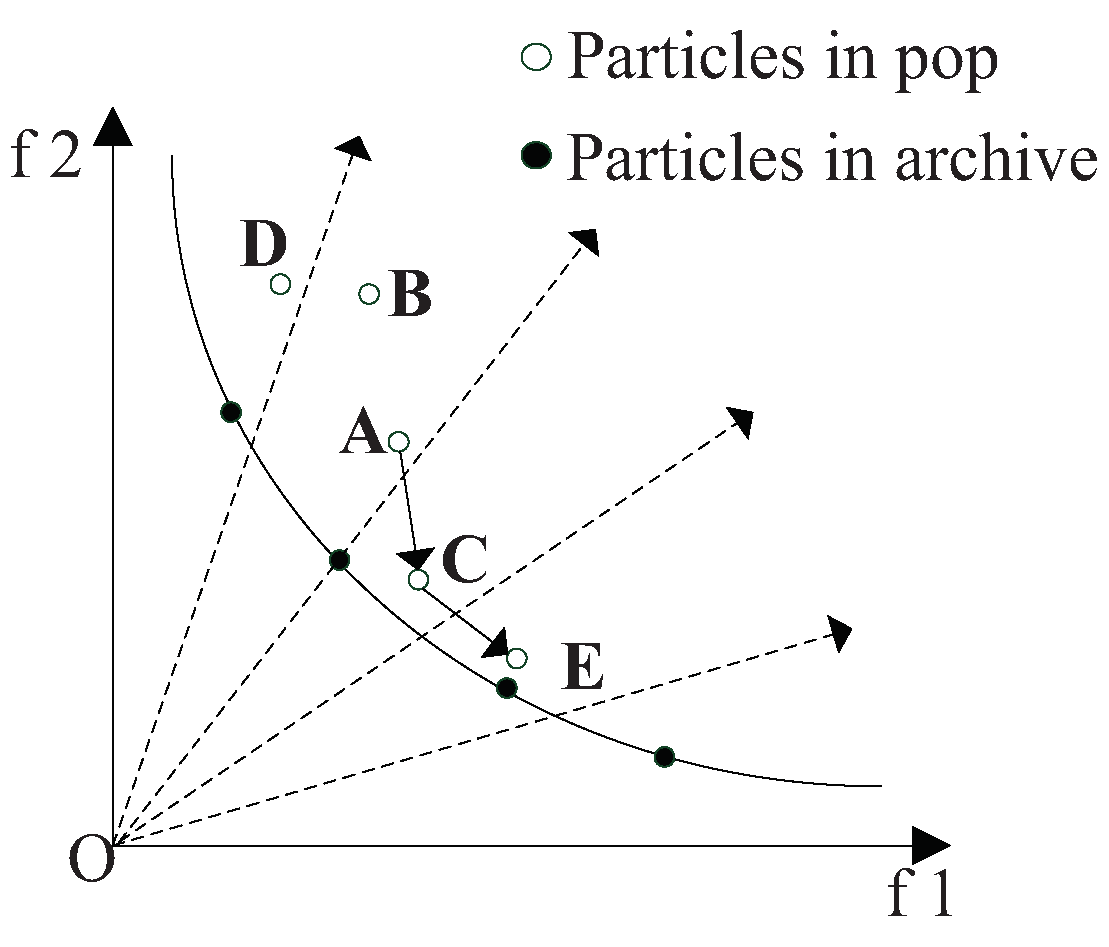N subproblems, and each particle is upadated based on the direction vectors. As shown in the Figure 5 and Figure 6, the dotted lines represent the direction vectors that partition the objective space. The solid lines represent the true frontier of the function. The solid dots represent the particles of elite archive. The hollow dots represent the particles of the population. In the update process, A is the position at the previous moment, B is the position at the current moment, and C is the position at the next moment. 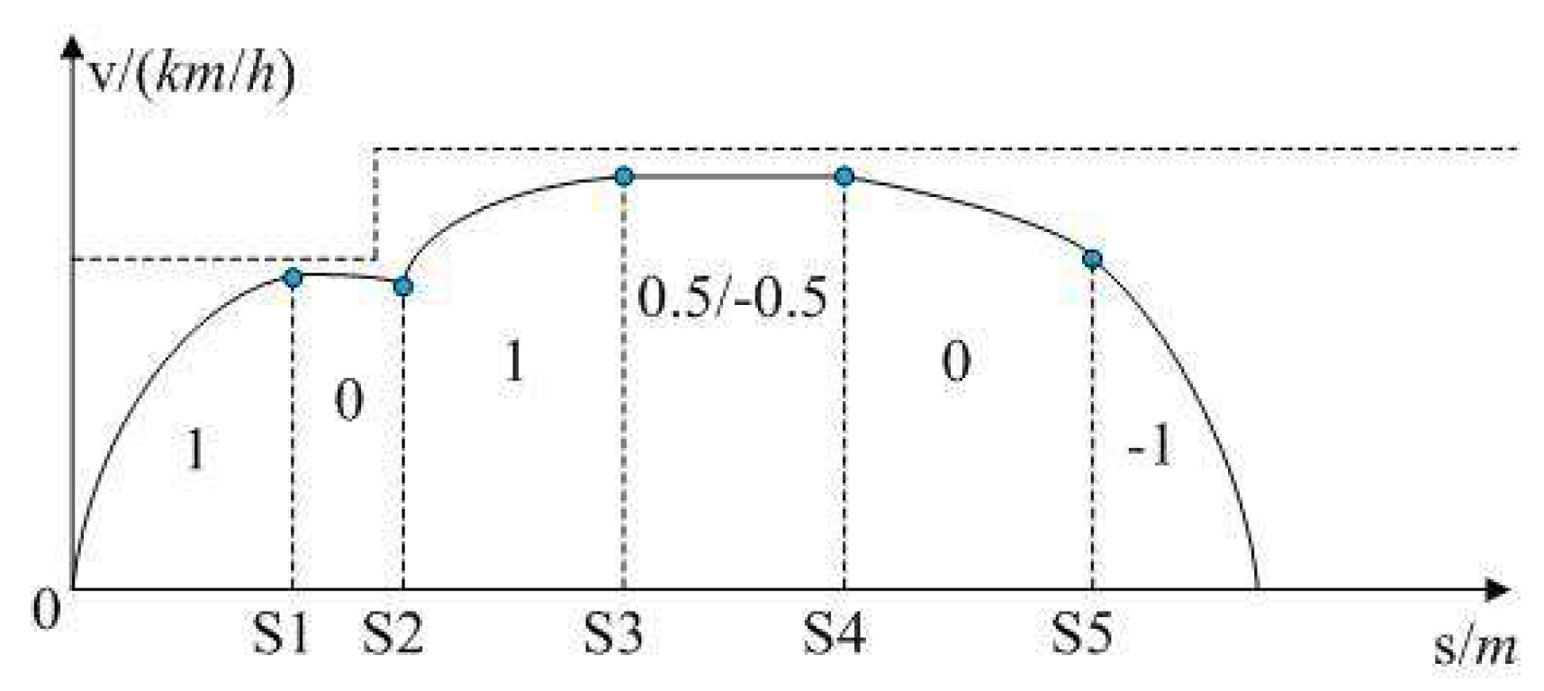The individual optimal value update mode of CLPSO is shown in Figure 5, and the optimal particle individual plays a guiding role in the search of the whole population. In order to update $pbest$, the decomposition method should be adopted to scale the multi-objective problem. Tchebycheff method is used to construct the aggregation function in this paper. By calculating the aggregate value of each particle, the binary tournament will remain throughout the binary tournament. The global optimal value update method for traditional PSO is shown in Figure 6. In Figure 6, the global optimal value of particle swarm is used to guide the development of particles, and the global optimal value of the particles is updated by using the information of the neighborhood particles.

Similar to traditional PSO, CLPSO tends to locally converge to an individual extreme value. In fact, the diversity of the population is obviously destroyed by the single learning optimization model. In this paper, an improved particle swarm optimization algorithm based on comprehensive learning strategy is proposed, which is denoted as ICLPSO. The flow diagram of this paper is shown in Figure 7.

In Figure 7, $P{c}_i$ is the learning probability, which determines whether it is updated based on template particles or not. As the number of iterations increases, the probability of particle swarm falling into local optimum increases gradually. In order to avoid that, the learning probability should also increase gradually. The formula of learning probability $P{c}_i$ is shown as follows:

$$\begin{array}{c}P{c}_i=0.05+0.45\frac{(exp\frac{10(i-1)}{N-1}-1)}{(exp(10)-1)}.\hfill \end{array}$$

(27)

If the i-th particle cannot be effectively optimized in continuous iteration (the refresh interval $gap$ generally is 2), this particle will learn by using formula 29 (CLPSO’s individual optimal value updating method). If $rand$ > $P{c}_i$, the corresponding dimension will learn from its own pbest, or it will learn from pbest of template particles. To obtain better diversity when handling complex MOP, the optimal particle among four random particles in template $f_i$ will be chosen as the template pbest.

4.2. Improved CLWOA

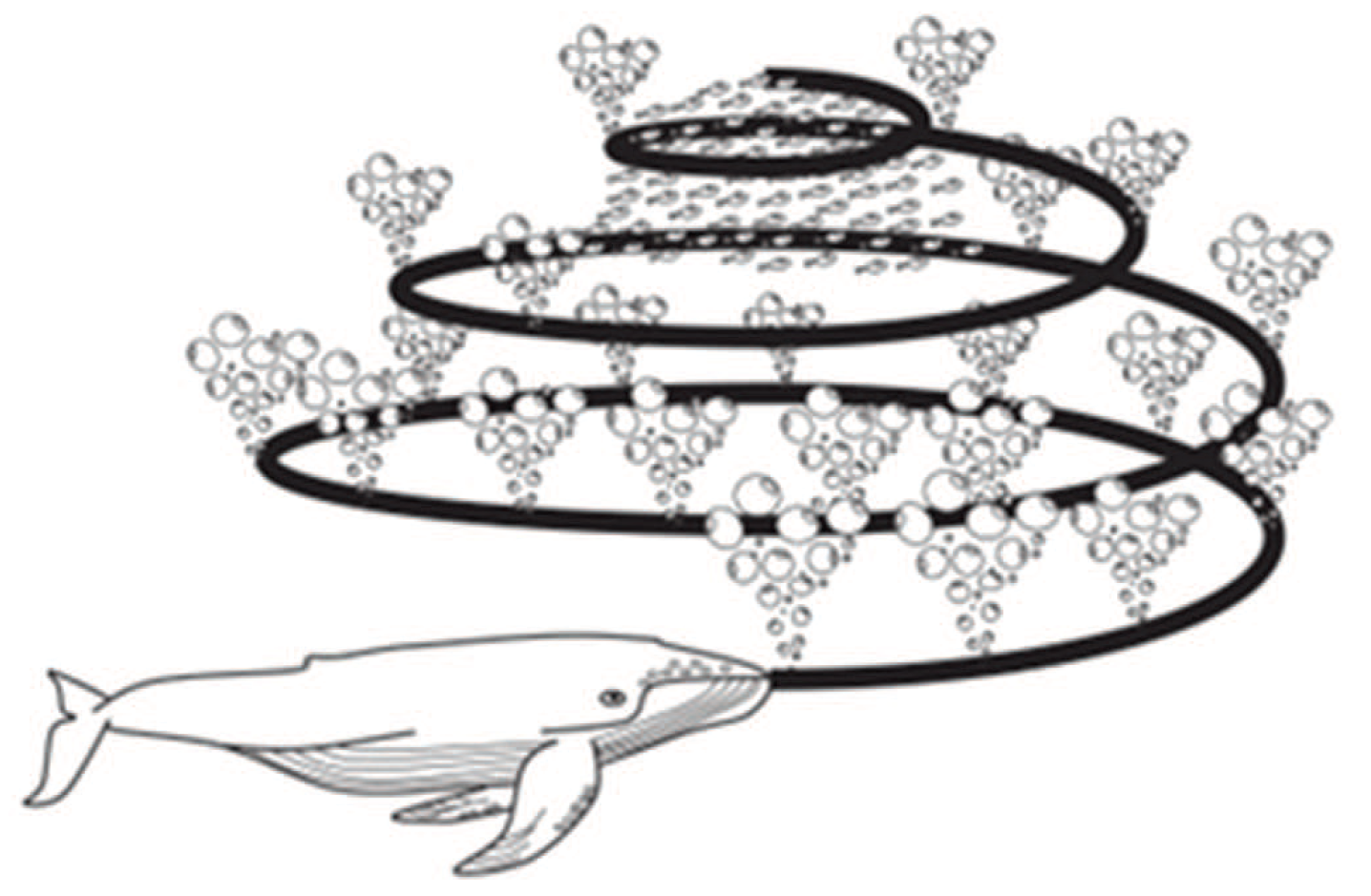
Whale optimization algorithm simulating whale foraging is one of the most efficient optimization algorithms, but it also has the disadvantage that it is easy to fall into local convergence in the later iteration [30]. Therefore, this paper proposes an improved WOA algorithm (ICLWOA) that contains both learning strategies. the specific improved measures are described below.

(1) Parameter adjustment based on chaos mapping

In the whale optimization algorithm, parameters A and C are important parameters, which affect the searching ability of the algorithm to some extent. In the traditional whale optimization algorithm, its parameters are generated in an excessively random manner, which will reduce the convergence speed of the algorithm and invalidate the search area in the later period of operation.

Chaos is a common phenomenon in nonlinear systems. Its change process seems to be chaotic, but, in fact, it has inherently regularity and can iterate over all states according to its own law within a certain range. The behavior of chaotic map is complex, which is similar to random motion. But compared with random motion, it has ergodicity, which can make up for the defect of random motion to achieve global optimization. Therefore, chaos theory is applied to WOA in this paper to improve WOA’s ability to explore and create new individuals [31].

$$\begin{array}{c}A=a(1-a)\hfill \end{array}$$

(28)

$$\begin{array}{c}C=2ran{d}^2·sin(\pi ·rand).\hfill \end{array}$$

(29)

By using chaos mapping to adjust parameters, the range of random search of parameters reduces and the regularity of parameters increases. In this way, on the basis of avoiding fall into local optimum in the search process, thus, avoiding the problems of slow convergence and invalid search area caused by random blind search.

(2) Boundary processing measures based on reverse learning

In the process of algorithm optimization, it is possible to ‘overflow’ the search scope when the individual updates. The general way to deal with that is to generate new random individuals who cross the boundary. However, if a large number of individuals exceeds the boundary, this results in the waste of search resources. When the updating position of the individual is out of bounds, if the individual position is randomly reset, the beneficial information obtained by the previous iteration of the individual will be lost. A reverse learning strategy can generate a reverse individual far away from the local optimal. Therefore, this paper uses the reverse learning strategy to effectively guide the whale to quickly return to the decision space which needs to be searched.

In the calculation process, if the i-th individual is over the boundary, then the reverse learning strategy is adopted for the previous individual $x_i^{pre}$. The specific formula is as follows:

$$\begin{array}{c}{x}_i^{op}=a_i+\beta \times (b_i-x_i^{pre}),i=1,2,\dots ,D,\hfill \end{array}$$

(30)

where $x_i^{op}$ is the reverse solution of the previous individual $x_i^{pre}$; $a_i$ and $b_i$ are respectively the maximum and minimum value of solution; $\beta \in \left[0,1\right]$, as a generalization coefficient, which can prevent individuals from excessive escape.

4.3. Improved Archive Mechanism

In the multi-objective optimization problem, it is impossible to directly compare the advantages and disadvantages of two individuals. In this paper, the Tchebycheff decomposition method is selected to quantify the multi-objective problem, and the aggregation function is used to compare the advantages and disadvantages of individuals. For the multi-objective optimization algorithm based on the decomposition method, the reference point $Z^{*}$ (elite individual) in the aggregation function plays a significant role in guiding the convergence direction of the population. In order to make better use of the information of each generation, the external elite archive set is used to record the beneficial information of the population after each population’s update. The elite archive set is recorded as Archive. The existing literature adds the updated non-dominant individuals from each generation to the archive mostly, so does this paper. As the number of iterations increases, more and more non-dominanted individuals are obtained. If all of them are kept in archive, it will greatly increase the computational burden of the algorithm [32]. Therefore, the elite archive set need to be kept within a certain size. In order to maintain the diversity of the whale elite archive set, this paper deletes the denser individuals by calculating the distance among individuals in archive. Traditional optimization algorithms generally adopt Euclidean distance, which is simple in definition and easy to calculate, as the distance measurement index. However, there are two weaknesses in Euclidean distance. First, the calculation of Euclidean distance depends on the dimensionality of variables, so its actual meaning is difficult to be explained. In addition, the distribution of samples is not taken into account when calculating Euclidean distance, so the correlation between variables cannot be measured. It is the straight-line distance between samples, so it is insufficient in solving the multivariate data analysis. Therefore, this paper uses the fusion distance which fuses Mahalanobis distance and Euclidean distance as the distance measurement index to maintain the archive scale. When the archive exceeds the predetermined scale, the fusion distance of each individual is calculated and the individual with small fusion distance is deleted until the scale of the archive is maintained at the predetermined value. The calculation formula of specific fusion distance is as follows:

$$\begin{array}{c}\left\{\begin{array}{c}{d}_{Mix}=\omega \times MD(X,Y)+\left(1-\omega \right)\times ED(X,Y)\\ \begin{array}{c}{C}_Y=\left[\begin{array}{cccc}{\rho }_{Y_1{Y}_1}& {\rho }_{Y_1{Y}_2}& \cdots & {\rho }_{Y_1{Y}_n}\\ {\rho }_{Y_2{Y}_1}& {\rho }_{Y_2{Y}_2}& \cdots & {\rho }_{Y_2{Y}_n}\\ ⋮& ⋮& \ddots & ⋮\\ {\rho }_{Y_n{Y}_{{}_1}}& {\rho }_{Y_n{Y}_2}& \cdots & {\rho }_{Y_{\mathrm{n}}{Y}_n}\end{array}\right]\hfill \\ \omega =\sqrt{1-\left|C_Y\right|}\hfill \end{array}\end{array}\right.,\hfill \end{array}$$

(31)

where $d_{Mix}$ represents fusion distance; $MD$ represents Mahalanobis distance; $C_Y$ represents the correlation confficient matrix of sample set Y; n represents the number of samples in Y; $Y_i\left(i=1,\cdots ,n\right)$ represents the samples in Y; $\rho$ represents the correlation confficient. Since the Mahalanobis distance takes into account the correlation between variables, it uses $\omega$ the weight with relevant information to fuse, while the Euclidean distance uses $1-\omega$ to fuse. Therefore, the fusion distance takes into account both the correlation between variables and the independence between variables [33].

Both PSO and WOA are optimization algorithms that the population mainly learns from the optimal individuals or some elite individuals. This optimization model of directional learning always has a relatively fixed evolutionary direction, which is not conducive to its maintenance of population diversity. Genetic algorithm has obvious advantages over PSO and WOA in maintaining population diversity, because it produces a large number of new solutions with great differences through selection, crossover and variation. Therefore, this paper introduces the genetic evolution mechanism into the optimization algorithm, so as to better maintain the population diversity of the optimization algorithm. However, if the genetic algorithm is introduced blindly and excessively, it will destroy the favorable information obtained by the long-term iterative learning of individuals on a large scale, which is not conducive to optimization. Based on the genetic algorithm and the elite archiving set, this paper proposes the following improvement strategy to prevent the aggregation of individuals in the population to maintain the diversity of the population, which is denoted as the improved elite archiving set mechanism (IESM). The specific steps are as follows:

Step 1: add the updated non-dominanted individuals in each generation to the elite archive set;

Step 2: determine whether the size $ES$ of the archive exceeds the predetermined value $E{S}_T$. If the condition is not true, skip step 3 and perform step 4.

Step 3: calculate the fusion distance between each individual to the archive (formula 34), and delete the individual with a smaller fusion distance until the size of the archive is maintained at a predetermined value;

Step 4: calculate the fusion distance radius $E{R}_{mix}$ of the elite individuals. The radius is the maximum distance between each individual in the elite archive set and the archive;

Step 5: test whether the number of individuals in the archive range $EN$ in the current population is greater than the threshold value $E{N}_T$. If the condition is not established, it indicates that there is no phenomenon of individuals gathering in the archive range in the population at this time. The fusion distance between the individual and the archive is less than the radius of the archive $E{R}_{M}ax$, which indicates that the individual is within the range of the elite archive set.

Step 6: select, cross recombination and mutation operation of genetic algorithm is used to reset the individuals that gather in the elite archive set, until there is no phenomenon that individuals gather in the archive range in the population.

Obviously, this mechanism has the following advantages:

(1) Keep the scale of archive little than the predetermined value ($ES\le E{S}_T$).

(2) Ensure that elite individuals are evenly distributed in the elite archive set.

(3) Suppress the archive ‘domination’ of the entire population by restricting the concentration of individuals in the archive ($EN\le E{N}_T$) to enhance the global convergence performance of the hybrid optimization algorithm.

4.4. Design of Hybrid Optimization Algorithm

PSO and WOA have a fixed optimization mode, and this optimization mode with certain optimization direction will damage the diversity of the population to a certain extent. Therefore, this paper designs a hybrid optimization algorithm which uses the elite archive as the medium of information exchange. The intelligent evolution process of its hybrid optimization algorithm is denoted as IEP, and the specific IEP flow chart is shown in Figure 8.

As shown in Figure 8, the step of improved CLHOA IEP is as follows:

Step 1:

(1) Initialize particle swarm (the size is N) and whale swarm (the size is N), including the velocity and position of each particle in the particle swarm, the Tchebycheff aggregation function value, and the individual optimal value, global optimal value of particle swarm, the Tchebycheff aggregation function value of each whale position in the whale group, the optimal whale position of the whale group $X^{*}$. The current iteration number is 1, and the number of weight vectors in each neighborhood is T.

(2) To initialize the common elite archive set of particle swarm and whale swarm, let archive = ∅ and initialize the reference point $z^{*}=(z_1^{*},z_2^{*},\dots ,z_m^{*})$, where $z_j^{*}=min\left(f_j\left(x\right)\right)$, $j=1,2,\dots ,m$ and m is the number of optimization objectives. A uniformly distributed weight vector set $\lambda eve{n}_{N\times m}$ is generated and used in the initial iteration calculation of ICLPSO and ICLWOA. let ${\lambda }^1=\lambda eve{n}_{N\times m}$, the elements in each row and column of the matrix $\lambda eve{n}_{N\times m}$ are uniformly distributed.

Step 2:

(1) Archive and two populations (particle swarm and whale swarm) are obtained.

(2) If the current iteration number is greater than 1, recalculate the reference points $z^{*}=(z_1^{*},z_2^{*},\dots ,z_m^{*})$, ${\lambda }^j$ and $B^j$. In the j-th iteration, the weight of the k-th optimization index of the i-th individual in the population is ${\lambda }^{j,i,k}$, $i\in \left\{1,2,\dots ,N\right\}$, $k,l\in \left\{1,2,\dots ,m\right\}$, and its calculation formula is as follows [34].

$$\begin{array}{c}{\lambda }^{j,i,k}=\frac{1}{f{\left(x^{j,i}\right)}^k-Z^{ref,k}}{\left({\displaystyle \sum _{l=1}^m}\frac{1}{f{\left(x^{j,i}\right)}^l-Z^{ref,l}}\right)}^{-1}.\hfill \end{array}$$

(32)

For any Pareto solution target $z^c=(z_1^c,z_2^c,\dots ,z_m^c)$ in a continuous Pareto front, the weight vector ${\lambda }^c$ is obtained according to the formula $\frac{1}{f\left(x\right)-Z^c}{\left({\displaystyle \sum _{ik=1}^m}\frac{1}{f\left(x\right)-Z^{c,ik}}\right)}^{-1}$. The optimal solution of the single objective subproblem corresponding to the weight vector ${\lambda }^c$ is the Pareto solution target $z^c$. Because Pareto front is not easily available, it is replaced by the nearest solution target $Z^{ref}$ to $z^c$ in the archive. The angles $〈{\lambda }^{j,i},{\lambda }^{j,ir}〉$ between ${\lambda }^{j,i}$ and the weight vectors ${\lambda }^{j,ir}$ of other individuals are calculated ($ir\in \left\{1,2,\dots ,N\right\}$), then take the smallest T weight vectors in $〈{\lambda }^{j,i},{\lambda }^{j,ir}〉$ to form the neighbor $B^{j,i}$ of ${\lambda }^{j,i}$.

(3) For each particle in the particle swarm, the particle velocity update process (Section 3.1) of ICLPSO is used to calculate the particle velocity and update the particle position. For each whale in the whale population, the whale location is updated according to the three stages of ICLWOA, and three additional learning strategies are adopted in the update process (Section 3.2).

(4) Update individual value and global optimal value based on the aggregate function’s value. If $g^{te}\left(x^{i,j}\right|{\lambda }^{i,j},z^{*})<g^{te}\left(X^{\prime }\right|{\lambda }^{i,j},z^{*})$ ($X^{\prime }$ could be $pbes{t}^i$, $gbest$ or $X^{*}$), the $X^{\prime }$ and $f\left(X^{\prime }\right)$ will be replaced by $x^{i,j}$ and $f\left(x^{i,j}\right)$.

(5) Obtain the Pareto front of the current particle population and the Pareto front of the whale population.

Step 3: information exchange based on the archive

(1) Expand the scale of the archive: extend the Pareto front of the current particle swarm and whale swarm to the elite archive. If there are the same individuals or dominated individuals, delete them until any two individuals in the elite archive are different and there is no dominated relationship.

(2) Maintain the size of the archive: if the size of the elite archive set exceeds the preset value, calculate the crowding distance between the elite solutions and delete the particle with the smallest crowding distance. If the size of the elite archive set still exceeds the preset value, continue to perform that until the size remains at the preset value. Fusion distance $d_{mix}$ is used as the index of distance measurement.

(3) Restrict the concentration of the population in the archive area: if there are individuals within the range of the archive in the population, the individuals within the elite archive set will be partially reset by selection, cross recombination, mutation operation of genetic algorithm until there is no individuals that are clustered within the range of archive. In order to better retain the favorable information obtained by the previous iteration of the individual, the object of the crossover recombination operation of the i-th individual $x^{i,j}$ in the j-th iteration needs to be selected from the individuals set $X{B}^{j,i}$ corresponding to the neighbor $B^{j,i}$ of its weight vector. Same as in step 2, the fusion distance $d_{mix}$ is adopted as the distance measurement index.

Step 4: if the maximum iteration number (or the maximum evaluation number) is reached, then terminate the algorithm and output the archive set, otherwise return Step 2.

5. The Experimental Simulation

5.1. Optimization Performance Analysis based on Standard Test Functions

In order to evaluate the performance of the proposed algorithm, six test functions were used in this paper [35,36]. The specific six test functions were two-objective function ZDT series (ZDT1 ZDT2 and ZDT3) and three-objective test function DTLZ series (DTLZ1 DTLZ2 and DTLZ7). ICLHOA (improved algorithm proposed in this paper) was compared with the results optimized by ICLWOA, ICLPSO, dMOPSO (multi-objective particle swarm optimization based on decomposition) [37], NSGAII (non-dominated sorting genetic algorithm II) [38] and MOEA/D (multi-objective evolutionary algorithm based on decomposition) [39]. ZDT1, ZDI2 and ZDI3 set 30 decision variables, and DTLZ1, DTLZ2 and DTLZ7 used seven, 12 and 22 decision variables, respectively. The specific parameters of the algorithm are as follows.

(1) ZDT function: the neighborhood size T was 10; the number m of targets was two; the number N of individuals was 100; the maximum number $F{E}_s$ of evaluation was 30,000.

(2) DTLZ function: the neighborhood size T was 10; the number m of targets is three; the number N of individuals was 200; the maximum number $F{E}_s$ of evaluation was 20,000.

In this paper, the inverse generation distance (IGD), which can represent the convergence and diversity of the algorithm, is used as the evaluation index. The calculation formula is shown in Formula (33).

$$\begin{array}{c}IGD=\frac{{\sum }_{i=1}^{\left|Pf\right|}d(P{f}_i,P{f}^{\prime })}{\left|Pf\right|},\hfill \end{array}$$

(33)

where $Pf$ is the set of uniform sampling points of the real Pareto front; $P{f}^{\prime }$ is the approximate Pareto solution set obtained by the algorithm to be tested; $\left|Pf\right|$ is the size of set $Pf$; $d\left(P{f}_i,P{f}^{\prime }\right)$ is the minimum distance between the i-th Pareto sampling point $P{f}_i$ and the Pareto solution set $P{f}^{\prime }$ [40].

The specific IGD values of each optimization algorithm are shown in

Table 1. Inverse generation distance (IGD) value of each optimization algorithm.

Function	ICLHOA	ICLWOA	ICLPSO	MOEA/D	NSGAII	dMOPSO
ZDT1	$7.8105\times {10}^{-4}$	$9.2897\times {10}^{-4}$	$1.3034\times {10}^{-3}$	$1.4151\times {10}^{-3}$	$1.7129\times {10}^{-3}$	$5.6937\times {10}^{-3}$
ZDT2	$8.3595\times {10}^{-4}$	$1.0828\times {10}^{-3}$	$3.8520\times {10}^{-3}$	$1.8149\times {10}^{-3}$	$2.0791\times {10}^{-3}$	$2.4068\times {10}^{-3}$
ZDT3	$4.0189\times {10}^{-3}$	$4.4719\times {10}^{-3}$	$3.8962\times {10}^{-3}$	$5.0144\times {10}^{-3}$	$1.0525\times {10}^{-2}$	$5.9348\times {10}^{-3}$
DTLZ1	$6.9047\times {10}^{-3}$	$8.3152\times {10}^{-3}$	$1.0439\times {10}^{-2}$	$1.0651\times {10}^{-2}$	$4.9473\times {10}^{-2}$	$2.0358\times {10}^{-2}$
DTLZ2	$4.3142\times {10}^{-3}$	$7.9516\times {10}^{-3}$	$6.5154\times {10}^{-3}$	$1.2257\times {10}^{-2}$	$4.2894\times {10}^{-3}$	$1.2976\times {10}^{-2}$
DTLZ7	$7.6342\times {10}^{-3}$	$7.8635\times {10}^{-3}$	$9.2405\times {10}^{-3}$	$5.3790\times {10}^{-2}$	$3.7759\times {10}^{-2}$	$3.9682\times {10}^{-2}$

, the PF (real Pareto front and approximate Pareto solution set) of each optimization algorithm is shown in Figure 9, Figure 10, Figure 11, Figure 12, Figure 13 and Figure 14, and the iterative convergence curves of IGD values of each optimization algorithm are shown in Figure 15.

It can be seen from Table 1 that, compared with the traditional algorithm and its improvement algorithm, ICLHOA had significant advantages over ZDT series of dual-objective test functions and DTLZ series of three-objective test functions; only in ZDT3, ICLHOA was slightly inferior to ICLPSO, and in DTLZ2, ICLHOA was slightly inferior to NSGAII. According to Figure 9, Figure 10, Figure 11, Figure 12, Figure 13 and Figure 14, the optimization results obtained by ICLHOA were closer to the real front of ZDT1, ZDT3, DTLZ2 and DTLZ7, and were distributed more evenly. Only in ZDT3 and DTLZ2, the optimization results of ICLHOA had no obvious advantages over ICLWOA and ICLPSO. According to Figure 16, compared with other optimization algorithms, ICLHOA not only found better IGD value, but also had a significantly faster convergence rate. Only on DTLZ2, the convergence rate of ICLHOA is slightly lower than that of NSGAII. In conclusion, ICLHOA had better optimization performance than other optimization algorithms in ZDT and DTLZ series test functions.

5.2. The Relevant Data and Simulation Platform of the Practical Example of Multi-Objective ATO

This paper selects the station area between new port in Lvshun and Tieshan town of Dalian rail transit line number 12 as the research object. The running section length was 2.94 km, with two long lower ramps and one long upper ramp. Dalian rail transit line number 12 is an urban rail transit line extending from Hekou station to new port in Lvshun, which has eight stations and seven operating zones. The specific basic train attributes are shown in

Table 2. Characteristics of the train.

Parameter Name	Parameter Characteristics
Train weight	211t
Maximum velocity	80 km/h
Marshalling form	2M2T
Mean acceleration	≥1.0 (m/s${}^2)$
Mean braking deceleration	≥1.0 (m/s${}^2)$
Rotary mass coefficient	0.06
Motor number	4
Adhesion coefficient	0.2
Power Voltage	1800 V

, and the ramp parameters and train speed limit are shown in Figure 16.

Most of the research on ATO for the traditional correlation algorithm is the offline simulation platform based on Matlab/Simulink. This simulation platform has serious defects. Because there is no real device or real controlled object in the simulation platform, the virtual simulation environment is a very ideal simulation environment, which is greatly different from the actual real-time and online ATO operation control environment. In order to solve the serious disconnection between the simulation environment and the actual situation, Germany dSPACE company developed a set of semi-physical real-time simulation platform based on Matlab/Simulink. The new dSPACE real-time simulation system contains some hardware objects such as controllers, which is also known as hardware-in-loop simulation (HILS). Because HLIS is able to safely and efficiently verify the optimal performance or control performance for electrical and control products, it can accelerate the breakthrough of the core algorithm, greatly improve the test efficiency, greatly reduce the development risk, greatly shorten the online time, and save the development cost as much as possible. After decades of development, HILS has been deeply favored by scientific research units and manufacturers all over the world. In China, many manufacturers (CRRC, China’s State Grid, China First Automobile) and higher teaching institutions (Shanghai Jiaotong University, National University of Defense Technology, Harbin Institute of Technology) have carried out scientific research in related fields based on HILS, and have achieved fruitful research results [41,42,43,44]. ATO has both optimization and control functions: the main processor unit (MPU) uses an optimization algorithm to optimize the train’s ideal target speed distance curve based on constraints such as line condition and optimization objectives such as expected running time. The traction control unit (TCU) uses a proper control algorithm to enable the train to track the target speed curve in real time. Therefore, the HILS platform contains two simulation parts: the upper optimization and the lower control. The upper optimization simulation aims to verify the optimization performance of optimizer (MPU), while the lower control simulation aims to verify the controllability of controller (TCU). The structure diagram of ATO HILS platform and the physical diagram of the simulation cabinet are shown in Figure 17 and Figure 18.

The automatic train operation HILS platform as shown in Figure 17, contains five kinds of actual hardware necessary for ATO, and two kinds of simulation hardware in place of actual hardware. Here is the specific actual hardware: sensors, conditioning circuit, signal processing unit, controller, optimizer, actuators. Among which, the controller (TCU) and optimizer (MPU) respectively contain the dSPACE board of the write-in control algorithm and optimization algorithm, which are the core equipment of ‘control loop’ and ‘optimized loop’; the sensors, conditioning circuit, signal processing unit are the equipment for connecting different equipment, collecting and processing different data information. The ‘control loop’ and ‘optimized loop’ maintain real-time communication with ‘dSPACE ATO simulation environment object’ through them, and use MVB (multifunction vehicle bus) as the communication protocol. The emulator and actuators are the two kinds of simulation hardware for ATO HILS platform, which is used for virtual replacement of the real environment or components not easily obtainable in real ATO, for example, running route, collecting electric network for traction, etc. The Emulator is used to provide the ATO simulation environment, for example, using rheostat to simulate the actual line. The Actuators are the actuating mechanism in ATO, mainly including inverter, rectifier and traction motors. Generally, their rated powers are $A_{s,p}$, which is the actuator simulation proportionality coefficient in a real circumstance and it is 1/2000 in this paper. In automatic train operation HILS platform, the control loop with the controller (TCU) as the core can be isolated. When the ‘control loop’ is isolated, corresponding control simulation module will be used in place of corresponding physical components as the hardware in ‘dSPACE ATO simulation environment object’ can be activated so as to virtualize the practical ATO control. In this paper, the HILS platform isolating the ‘control loop’ that contains the physical hardware component, is marked as ICL-HILS, and the HILS platform retaining the ‘control loop’ that contains the physical hardware components as RCL-HILS.

In Figure 18, the simulation cabinet contains four kinds of hardware devices of HILS platform: ‘emulator’ provides ‘dSPACE ATO simulation environment object’ to the HILS platform, which includes various related models, such as the vehicle dynamics model, wheel and rail model, line model, accurate braking model, traction transformer model, traction rectifier model, traction inverter model, traction motor model, etc; ‘conditioning circuit’ can regulate electrical signals appropriately; ‘signal processing unit’ can adjust the network signal accordingly; ‘controller (TCU)’ can apply ATO real-time control instructions according to the actual situation. The HILS platform also has many external service devices, such as optimizer (MPU), speed sensor, current sensor, permanent magnet synchronous motor (PMSM), AC–DC converter, DC–AC converter, etc.

As the HILS platform contains a large number of real train-borne equipment, it can truly reflect the real-time data interactive, conversion and processing in the actual ATO. Therefore, HILS environment completely overcomes the various defects that Matlab/simulink simulation cannot consider the sensor sampling accuracy, can only ignore the disturbance imposed by signal transmission delay and imposes an overly idealistic disturbance. The specific differences among Matlab/simulink, ICL-HILS and RCL-HILS are shown in

Table 3. Differences of three different simulation platforms.

Differences	Matlab/Simulink	ICL-HILS	RCL-HILS
Obtain real-time speed	Calculated by simulation	Real measurement	Real measurement
Sampling accuracy	Completely ignored	True reflection	True reflection
Signal delays and errors	Completely ignored	True reflection	True reflection
Obtain real-time acceleration	Calculated by simulation	Calculated by simulation	Real measurement
TCU controller performance	Ideal	Ideal	True reflection
actuators control performance	Ideal	Ideal	True reflection
Difference from the real ATO	High degree	Middle degree	Low degree
Reference value of actual ATO	less value	certain value	Considerable value

.

5.3. The Optimization Result of Multi-Objective ATO Actual Example

Based on the metro train of Dalian rail transit line number 12 and the running line between the new port station in Lvshun and Tieshan town station area, Matlab/simulink, ICL-HILS and RCL-HILS are adopted, and ICLHOA, ICLWOA, ICLPSO, dMOPSO [36], NSGAII [37] and MOEA/D [38] are respectively used to find optimal solutions. The algorithms mentioned above are written into the optimization model of Matlab/simulink and the chips of optimizer (MPU) of ICL-HILS and RCL-HIL. The simulation environment of the algorithm is the same, including the basic settings of algorithm parameters and the configuration of software and hardware, and the specific configuration is described below: The population size is 100; the number of iterations is 150; configuration of Matlab/simulink platform is the same (Matlab GUI 2016a, CPU Core i7, Windows 10); configuration of HILS platform is the same (the core chip of the controller is ‘TMS320F28335’, the processor of emulator is ‘DS1006’). The controller of HILS platform has identical control algorithms, and also chooses fuzzy PID (fuzzy proportion integration differentiation) or MPC as control algorithms, which is good in control performance and strong in universality. The optimal solution must satisfy the following conditions: the train’s instantaneous speed must not exceed the speed limit; the train must complete the journey; the running time error is less than 0.2 seconds. When the planned running time is 180 s, the velocity ideal trajectory profile, control sequence distance curve and optimization results obtained by different algorithms are shown in Figure 19, Figure 20, Figure 21, Figure 22, Figure 23 and Figure 24 and

Table 4. Optimization results of velocity ideal trajectory profile obtained by different algorithms in Matlab/simulink.

Algorithm	Actual Running Time (s)	Energy Consumption (kJ)	Comfort Level (m/s${}^2)$	Parking Error (m)
ICLHOA	180.0373	103,173	5.5341	0.0849
ICLWOA	180.0685	107,974	7.2205	0.0851
ICLPSO	180.0478	116,353	6.9609	0.0893
MOEA/D	180.1144	119,237	8.3855	0.0958
NSGAII	180.0943	120,778	7.3619	0.1021
dMOPSO	180.0808	128,385	8.2057	0.0939

,

Table 5. Optimization results of velocity ideal trajectory profile obtained by different algorithms in isolating ‘control loop’ containing physical hardware devices (ICL)-hardware-in-the-loop simulation (HILS).

Algorithm	Actual Running Time (s)	Energy Consumption (kJ)	Comfort Level (m/s${}^2)$	Parking Error (m)
ICLHOA	180.0507	101,170	5.6074	0.0897
ICLWOA	180.1145	102,553	6.4275	0.0906
ICLPSO	180.0874	109,457	6.4117	0.0930
MOEA/D	180.1155	106,635	7.3925	0.0943
NSGAII	180.1307	114,899	8.8007	0.0994
dMOPSO	180.1519	120,391	8.6329	0.1012

and

Table 6. Optimization results of velocity ideal trajectory profile obtained by different algorithms in retaining ‘control loop’ containing physical hardware devices (RCL)-HILS.

Algorithm	Actual Running Time (s)	Energy Consumption (kJ)	Comfort Level (m/s${}^2)$	Parking Error (m)
ICLHOA	180.0828	110,469	5.0704	0.1831
ICLWOA	180.1343	125,541	6.5868	0.2004
ICLPSO	180.1288	120,939	5.6703	0.2029
MOEA/D	180.1106	124,271	7.1907	0.2138
NSGAII	180.1912	126,219	6.4731	0.1942
dMOPSO	180.1797	132,039	7.0781	0.2016

.

Figure 21, Figure 22, Figure 23 and Figure 24 show that in the real-time simulation of ICL-HILS and RCL-HILS, the power was switched on, the pantograph was raised, and the circuit breaker was normally closed. At the same time, the dSPACE simulator was in the working state (the dSPACE button was pressed and the procedure button is waiting to be pressed), the human–computer interaction signal was normal (the design button was green), and the parameters cannot be changed (the parameters button was red). Table 3, Table 4 and Table 5 show that, based on Matlab/Simulink, ICL-HILS and RCL-HILS, when the planned running time was 180 s and the simulation operation environment was the same, the optimal solution obtained by ICLHOA was superior to other optimization algorithms, and the three indicators, such as energy saving, punctuality and comfort have been improved to a considerable extent. The running line selected in this paper was located in the hilly area of economic and technological development zone in Lvshun, Dalian, and hilly was the typical geomorphologic feature in Dalian. In such a terrain, the control sequence needs to be concise and able to use the large downhill for acceleration and large uphill for deceleration, as much as possible, in order to reduce turbulence, save energy and improve punctuality. As can be seen from Figure 25, ICLHOA can obtain extremely smooth target velocity distance curve under the three simulation platforms mentioned above, and can maximize the use of long uphill and long downhill slopes. As can be seen from Figure 20, Figure 22, and Figure 24, the control sequence obtained by ICLHOA was the most concise, which can avoid unnecessary manipulation to the greatest extent As can be seen from Figure 19, Figure 21, and Figure 23, the target speed distance curve obtained by ICLHOA was the smoothest, compared with other algorithms, which enables the train to maintain an appropriate speed more smoothly. This advantage was particularly evident in the 12 enlarged areas of the three figures. The control algorithm (fuzzy PID or model predictive control) used is written in the kernel chip of controller (TCU) of ‘control loop’ in RCL-HILS. Under RCL-HILS, the target velocity distance curve obtained by partial optimization algorithm can be tracked and controlled by the controller. When the planned running time was 180 s, the actual velocity distance curve and corresponding control results obtained by partial tracking control algorithms under RCL-HILS are shown in

Table 7. The tracking model predictive control (MPC) results of the velocity ideal trajectory profile obtained by partial algorithms under RCL-HILS.

Algorithm	Actual Running Time (s)	Energy Consumption (kJ)	Comfort Level (m/s${}^2)$	Parking Error (m)
ICLHOA	180.1174	124,144	46.5479	0.2097
ICLWOA	180.2040	150,293	55.6232	0.3209
ICLPSO	180.1973	140,713	52.1124	0.2548
MOEA/D	180.1641	147,030	60.9828	0.3522

and

Table 8. The tracking fuzzy PID results of the velocity ideal trajectory profile obtained by partial algorithms under RCL-HILS.

Algorithm	Actual Running Time (s)	Energy Consumption (kJ)	Comfort Level (m/s${}^2)$	Parking Error (m)
ICLHOA	180.1391	125,944	48.1066	0.2188
ICLWOA	180.2095	162,183	59.4708	0.3721
ICLPSO	180.2014	153,165	61.9248	0.4085
MOEA/D	180.1766	156,847	65.9417	0.3926

and Figure 26 and Figure 27.

As can be seen from Figure 26 and Figure 27, whichever control algorithm is adopted (MPC or fuzzy PID), when RCL-HILS real-time tracking control is applied, the power supply was switched on, the pantograph was raised, and the circuit breaker is normally closed. At the same time, the dSPACE simulator was in the simulation state (the ‘dSPACE’ button is pressed and the ‘reality’ button was waiting to be pressed), the design parameters cannot be changed in the tracking control state (the ‘design’ button was white) and the given parameters cannot be changed (the ‘parameters’ button was red). As can be seen from the four enlarged areas in Figure 26 and Figure 27, whichever control algorithm was adopted (MPC or fuzzy PID), the tracking control speed curve corresponding to ICLHOA was optimal compared with other algorithms. Because the ideal curve obtained by ICLHOA was relatively smooth, it was easier to avoid the phenomenon of unstable speed control caused by signal transmission delay, limited control performance and uncertain disturbance in the simulation process. The reason is that the ICLHOA optimizer (MPU) kernel chip has more powerful optimization ability to find a more optimized target speed distance curve, and the target speed distance curve is smoother, which is easy to be tracked by a tracking control algorithm. It can be seen from Table 6 that, in terms of the actual running time, ICLWOA and ICLPSO algorithms barely reached the standard under RCL-HILS, and the running time error was about 0.2 s; NSGAII and dMOPSO algorithms can reach the standard under ICL-HILS, but they cannot be tracked and controlled under RCL-HILS due to insufficient margin, and the running time errors were 0.1912 s and 0.1797 s, respectively. If the comfort level was limited below 175 (m/s${}^2)$, the target velocity trajectory obtained by MOEA/D algorithm cannot be tracked and controlled under the current conditions. To sum up, ICLHOA was more suitable for solving ATO multi-objective train operation process optimization problem, and the actual train operation process results can meet the expected assumptions even under RCL-HILS. Furthermore, a large number of control algorithms (such as MPC and fuzzy PID) are suitable to being used as tracking control algorithms for ATO. However, some control algorithms (such as MPC) with good tracking performance are more recommended. Compared with fuzzy PID, more ideal tracking results is obtained by adopted MPC (as shown in Figure 26 and Figure 27 and Table 7 and Table 8), the fluctuation of velocity was more restrained (as shown in the four enlarged areas in Figure 26 and Figure 27, especially the enlarged area which distance interval was [2400,2800]).

At running time arrangement plan, the planned running time of the simulation line was 180 s in the flat time period (the traffic is relatively ideal, such as weekday morning 9:00–11:00 h), the planned running time is 175 s during peak time period (the traffic is relatively nervous, such as weekday morning 6:00–8:00 h). If the planned running time was 175 s, there were still similar simulation conclusions under the same calculation conditions, which further indicates that ICLHOA is more suitable for solving ATO multi-objective train running process optimization problem. Under RCL-HILS, the optimal target velocity distance curves and their corresponding optimization results obtained by different algorithms and the actual velocity distance curves and their corresponding control results obtained by some algorithms through tracking MPC are shown in Figure 28 and Figure 29 and

Table 9. The tracking MPC results of the velocity ideal trajectory profile obtained by partial algorithms under RCL-HILS (peak time period).

Algorithm	Actual Running Time (s)	Energy Consumption (kJ)	Comfort Level (m/s${}^2)$	Parking Error (m)
ICLHOA	175.0711	133,602	43.8712	0.1741
ICLWOA	175.1093	137,920	49.5864	0.2344
ICLPSO	175.1334	143,797	55.0125	0.2587
MOEA/D	175.1504	141,858	54.8821	0.3613

and

Table 10. Optimization results of velocity ideal trajectory profile obtained by different algorithms in RCL-HILS (peak time period).

Algorithm	Actual Running Time (s)	Energy Consumption (kJ)	Comfort Level (m/s${}^2)$	Parking Error (m)
ICLHOA	175.0497	119,559	5.7081	0.1097
ICLWOA	175.0741	120,212	6.2151	0.1681
ICLPSO	175.0940	125,718	6.5618	0.1770
MOEA/D	175.1043	124,271	6.6327	0.2077
NSGAII	175.1709	122,442	6.4983	0.1893
dMOPSO	175.1465	120,156	7.2121	0.1580

.

In order to verify that the improved algorithm (ICLHOA) in this paper has good universality and better practical optimization effect, multiple ATO scenarios are given as the optimized object for ICLHOA and some comparison algorithms, the optimization effect as shown in Table 4, Table 5, Table 6, Table 7, Table 8, Table 9 and Table 10 and Figure 19, Figure 20, Figure 21, Figure 22, Figure 23, Figure 24, Figure 25, Figure 26, Figure 27, Figure 28 and Figure 29. Obviously, in some different types of ATO scenarios (different simulation environments, different control algorithms, different control algorithms, different ATO requirements), compared with these comparison algorithms (ICLWOA, ICLPSO, dMOPSO, NSGAII and MOEA/D), ICLHOA obtained more ideal optimization results. This shows that ICLHOA is an all-purpose algorithm with good practical optimization effect for ATO velocity ideal trajectory profile optimization design problem.

6. Conclusions

ATO velocity ideal trajectory profile optimization design problem is a complex optimization problem that needs to take into account the energy consumption, running time, comfort and parking accuracy, which is not easy to obtain the ideal optimization solution. In order to, in any circumstance, obtain the ATO velocity ideal trajectory profile with a excellent effect for the whole optimization, the scientific researchers relating to it are required to provide an optimized suitable for most ATO velocity ideal trajectory profile optimization design problems, and having a very good effect for optimized algorithm. However, as far as the status quo is concerned, there are three types of problems needing urgent solution.

(1) The optimization performance of the optimized algorithm used is not good enough, or is unable to find the ATO velocity ideal trajectory profile with better comprehensive performance indicators, or is able to find it but which is not easy to be tracked and controlled. There are two possibilities, i.e., the design of the optimization algorithm itself is not excellent, or it is not suitable for finding an excellent ATO velocity ideal trajectory profile.

(2) The optimization algorithm used is strongly restrictive, with which some ATO velocity ideal trajectory profiles with special characteristics can be designed, for example, the mileage of driving route cannot be greater than the threshold, and it is only limited to low-speed light rail or metro, there cannot be too many long and big slope section on the route, it is not suitable for such route that is easy to get jammed, etc.

(3) The optimization algorithm used is poor in optimization efficiency during practical application. The actual ATO needs to consider the sampling accuracy, signal transmission delay or packet loss, as well as various unstable factors in the course of control. However, the simply simulated ATO model to be optimized cannot truly reflect these complicated circumstances. Actually, it is a special case in which a real ATO is simplified. This leads to some designed and improved optimization algorithms having no expected optimization effect in practical application.

In order to solve the above three kinds of problems more effectively, a thorough improvement has to be made to the optimization algorithm itself for the ATO velocity ideal trajectory profile optimization design problem so as to consider both the actual optimization performance and application scope. Therefore, ICLHOA proposed in this paper is a multi-objective hybrid optimization algorithm with excellent global optimization performance. ICLHOA combines the improved WOA and the improved PSO (ICLPSO and ICLWOA) which adopts the comprehensive learning strategy, and also uses the improved elite archive set mechanism and intelligent evolution process.

The advantages of ICLHOA are as follows:

(1) ICLPSO adopts a variety of particle optimization models to avoid the destruction of population diversity caused by a single model.

(2) In ICLWOA, chaos mapping operation is introduced to avoid random and blind search in the process of iterative calculation. Reverse learning is carried out for the individuals who cross the boundary, so as to better retain the beneficial information in the iterative process.

(3) Improved elite archive set mechanism is used to store the non-dominant solution in the optimization process, and the fusion distance is used to ensure the diversity of the elite archiving set.

(4) The dual-population parallel evolution process, which uses the elite archive set as the information communication medium, can greatly improve the computational efficiency and improve the global convergence performance of ICLHOA.

According to the Matlab/simulink results and ATO HILS (hardware-in-the-loop simulation) results, compare with the traditional intelligent optimization algorithm and its improvement algorithm, ICLHOA has better global convergence performance, so it can get more ideal optimization results. In this paper, two different autonomous driving scenarios (the planned running times are 180 s and 175 s) are taken into account, and ICLHOA is optimized to obtain more ideal target velocity trajectory, and the tracking control effect under RCL-HILS is very ideal. This shows that ICLHOA is able to find a more ideal solution for complex ATO practical problems, compared with the traditional optimization algorithm and its improved algorithm, thus it has stronger applicability.

References

1. Chang, C.S.; Xu, D.Y. Differential evolution based tuning of fuzzy automatic train operation for mass rapid transit system. IEEE Proc. Electr. Power Appl. 2000, 147, 206–212. [Google Scholar] [CrossRef]
2. Cai, B.; Sheng, Z.; Shang, G.W.; Sun, J. Train trajectory optimization with dynamic headway. In Proceedings of the 36th Chinese Control Conference, Dalian, China, 26–28 July 2017; pp. 9920–9925. [Google Scholar]
3. Adrián, F.-R.; Antonio, F.-C.; Asunción, P.C.; Marı’a, D.; Tad, G. Design of Robust and Energy-Efficient ATO Speed Profiles of Metropolitan Lines Considering Train Load Variations and Delays. IEEE Trans. Automat. Sci. Eng. 2015, 16, 2061–2071. [Google Scholar]
4. María, D.; Antonio, F.-C.; Asunción, P.C.; Ramón, R.P. Energy Savings in Metropolitan Railway Substations Through Regenerative Energy Recovery and Optimal Design of ATO Speed Profiles. IEEE Trans. Automat. Sci. Eng. 2012, 9, 496–504. [Google Scholar]
5. Gu, Q.; Meng, Y.; Ma, F. Energy saving for automatic train control in moving block signaling system. China Commun. Suppl. 2014, 11, 12–22. [Google Scholar] [CrossRef]
6. Gu, Q.; Tang, T.; Cao, F.; Song, Y. Energy-Efficient Train Operation in Urban Rail Transit Using Real-Time Traffic Information. IEEE Trans. Intell. Transp. Syst. 2014, 15, 1216–1233. [Google Scholar] [CrossRef]
7. Gu, Q.; Tang, T.; Ma, F. Energy-Efficient Train Tracking Operation Based on Multiple Optimization Models. IEEE Trans. Intell. Transp. Syst. 2016, 17, 882–892. [Google Scholar] [CrossRef]
8. Bai, Y.; Tin, K.H.; Mao, B.; Ding, Y.; Chen, S. Energy-Efficient Locomotive Operation for Chinese Mainline Railways by Fuzzy Predictive Control. IEEE Trans. Intell. Transp. Syst. 2014, 15, 938–948. [Google Scholar] [CrossRef]
9. Gao, S.; Dong, H.; Chen, Y.; Ning, B.; Chen, G. Approximation-Based Robust Adaptive Automatic Train Control: An Approach for Actuator Saturation. IEEE Trans. Intell. Transp. Syst. 2013, 14, 1733–1742. [Google Scholar] [CrossRef]
10. Jiateng, Y.; Chen, D.; Li, L. Intelligent Train Operation Algorithms for Subway by Expert System and Reinforcement Learning. IEEE Trans. Intell. Transp. Syst. 2014, 15, 2561–2571. [Google Scholar]
11. Zhou, Y.; Tao, X. Robust Safety Monitoring and Synergistic Operation Planning Between Time and Energy-Efficient Movements of High-Speed Trains Based on MPC. IEEE Access 2018, 6, 17377–17390. [Google Scholar] [CrossRef]
12. Meng, J.; Xu, R.; Li, D.; Chen, X. Combining the Matter-Element Model With the Associated Function of Performance Indices for Automatic Train Operation Algorithm. IEEE Trans. Intell. Transp. Syst. 2019, 20, 253–263. [Google Scholar] [CrossRef]
13. Song, Y.; Song, W. A Novel Dual Speed-Curve Optimization Based Approach for Energy-Saving Operation of High-Speed Trains. IEEE Trans. Intell. Transp. Syst. 2016, 17, 1564–1575. [Google Scholar] [CrossRef]
14. Shangguan, W.; Yan, X.; Cai, B.; Wang, J. Multiobjective Optimization for Train Speed Trajectory in CTCS High-Speed Railway With Hybrid Evolutionary Algorithm. IEEE Trans. Intell. Transp. Syst. 2015, 16, 2215–2225. [Google Scholar] [CrossRef]
15. Yang, X.; Li, X.; Ning, B.; Tang, T. A Survey on Energy-Efficient Train Operation for Urban Rail Transit. IEEE Trans. Intell. Transp. Syst. 2015, 17, 2–13. [Google Scholar] [CrossRef]
16. Saban, G.; Halife, K. A novel parallel multi-swarm algorithm based on comprehensive learning particle swarm optimization. Eng. Appl. Artif. Intell. 2015, 45, 33–45. [Google Scholar]
17. Huang, V.L.; Suganthan, P.N.; Liang, J.J. Comprehensive learning particle swarm optimizer for solving multiobjective optimization problems: Research Articles. Int. J. Intell. Syst. 2006, 21, 209–226. [Google Scholar] [CrossRef]
18. Ling, Y.; Zhou, Y.; Luo, Q. Lévy Flight Trajectory-Based Whale Optimization Algorithm for Global Optimization. IEEE Access 2017, 5, 6168–6186. [Google Scholar] [CrossRef]
19. Sun, W.; Wang, J. Elman Neural network Soft-sensor Model of Conversion Velocity in Polymerization Process Optimized by Chaos Whale Optimization Algorithm. IEEE Access 2017, 5, 13062–13076. [Google Scholar] [CrossRef]
20. Zhang, C.; Fu, X.; Leo, P.L.; Peng, S.; Xie, M. Synthesis of Broadside Linear Aperiodic Arrays With Sidelobe Suppression and Null Steering Using Whale Optimization Algorithm. IEEE Antennas Wirel. Propag. Lett. 2018, 17, 347–350. [Google Scholar] [CrossRef]
21. Cale, J.; Johnson, B.; Dall’Anese, E.; Young, P.; Duggan, G.; Bedge, P.; Zimmerle, D.; Holton, L. Mitigating Communication Delays in Remotely Connected Hardware-in-the-loop Experiments. IEEE Trans. Ind. Electron. 2018, 65, 9739–9748. [Google Scholar] [CrossRef]
22. Hasanzadeh, A.; Edrington, C.S.; Stroupe, N.; Bevis, T. Real-Time Emulation of a High-Speed Microturbine Permanent-Magnet Synchronous Generator Using Multiplatform Hardware-in-the-Loop Realization. IEEE Trans. Ind. Electron. 2013, 61, 3109–3118. [Google Scholar] [CrossRef]
23. Riad, A.; Toufik, R.; Djamila, R.; Abdelmounaïm, T. Robust nonlinear predictive control of permanent magnet synchronous generator turbine using Dspace hardware. Int. J. Hydrog. Energy 2016, 41, 21047–21056. [Google Scholar]
24. Yu, M.; Tang, X.; Lin, Y.; Wang, X. Diesel engine modeling based on recurrent neural networks for a hardware-in-the-loop simulation system of diesel generator sets. Neurocomputing 2018, 283, 9–19. [Google Scholar] [CrossRef]
25. Cheng, J.; Howlett, P. Application of critical velocities to the minimisation of fuel consumption in the control of trains. Automatica 1992, 28, 165–169. [Google Scholar]
26. Howlett, P.; Cheng, J. Optimal driving strategies for a train on a track with continuously varying gradient. J. Aust. Math. Soc. 1997, 38, 388–410. [Google Scholar] [CrossRef] [Green Version]
27. Lu, H.; Zhang, M.; Fei, Z.; Mao, K. Multi-Objective Energy Consumption Scheduling in Smart Grid Based on Tchebycheff Decomposition. IEEE Trans. Smart Grid 2015, 6, 2869–2883. [Google Scholar] [CrossRef]
28. Mirjalili, S.; Lewis, A. The Whale Optimization Algorithm. Adv. Eng. Softw. 2016, 95, 51–67. [Google Scholar] [CrossRef]
29. Gao, L.; Hailu, A. Comprehensive Learning Particle Swarm Optimizer for Constrained Mixed-Variable Optimization Problems. Int. J. Comput. Int. Sys. 2010, 6, 832–842. [Google Scholar] [CrossRef]
30. Kaur, G.; Arora, S. Chaotic Whale Optimization Algorithm. J. Comput. Des. Eng. 2018, 5, 275–284. [Google Scholar] [CrossRef]
31. Dumitriu, T. A novel hybrid approach of Evolutionary Algorithm based on Imperialist Competitive Algorithm. In Proceedings of the 19th International Conference on System Theory, Control and Computing, Cheile Gradistei, Romania, 14–16 October 2015; pp. 140–146. [Google Scholar]
32. Dharmbir, P.; Aparajita, M.; Gauri, S.; Vivekananda, M. Application of chaotic whale optimisation algorithm for transient stability constrained optimal power flow. IET Sci. Meas. Technol. 2006, 24, 83–88. [Google Scholar]
33. Liu, G.; Wang, X. Fault diagnosis of diesel engine based on fusion distance calculation. In Proceedings of the Advanced Information Management, Communicates, Electronic & Automation Control Conference, Chongqing, China, 24–26 March 2017; pp. 1621–1627. [Google Scholar]
34. Miettinen, K. Nonlinear Multiobjective Optimization; Kluwer Academic Publishers: Norwell, MA, USA, 2017. [Google Scholar]
35. Zitzler, E.; Deb, K.; Thiele, L. Comparison of Multiobjective Evolutionary Algorithms: Empirical Results. Evolut. Comput. 2000, 8, 173–195. [Google Scholar] [CrossRef] [Green Version]
36. Deb, K.; Thiele, L.; Laumanns, M.; Eckart, Z. Scalable multi-objective optimization test problems. Congr. Evolut. Comput. IEEE 2002, 1, 825–830. [Google Scholar]
37. Peng, H.; Li, R.; Cao, L.; Li, L. Multiple Swarms Multi-Objective Particle Swarm Optimization Based on Decomposition. Proced. Eng. 2011, 15, 3371–3375. [Google Scholar] [Green Version]
38. Zhang, Q.; Li, H. MOEA/D: A Multiobjective Evolutionary Algorithm Based on Decomposition. IEEE Trans. Evolut. Comput. 2008, 11, 712–731. [Google Scholar] [CrossRef]
39. Kalyanmoy, D.; Amrit, P.; Sameer, A.; Meyarivan, T. A fast and elitist multiobjective genetic algorithm: NSGA-II. IEEE Trans. Evolut. Comput. 2002, 6, 182–197. [Google Scholar] [Green Version]
40. Li, H.; Zhang, Q. Multiobjective Optimization Problems With Complicated Pareto Sets, MOEA/D and NSGA-II. IEEE Trans. Evolut. Comput. 2009, 13, 284–302. [Google Scholar] [CrossRef]
41. Yu, S.; Han, J.; Qu, Z.; Yang, Y. A Force and Displacement Compensation Method Toward Divergence and Accuracy of Hardware-in-the-Loop Simulation System for Manipulator Docking. IEEE Access 2018, 6, 35091–35104. [Google Scholar] [CrossRef]
42. Luo, G.; Zhang, R.; Chen, Z.; Tu, W.; Zhang, S.; Ralph, K. A Novel Nonlinear Modeling Method for Permanent-Magnet Synchronous Motors. IEEE Trans. Ind. Electron. 2016, 63, 6490–6498. [Google Scholar] [CrossRef]
43. Zhang, H.; Zhang, Y.; Yin, C. Hardware-in-the-Loop Simulation of Robust Mode Transition Control for a Series-Parallel Hybrid Electric Vehicle. IEEE Trans. Veh. Technol. 2016, 63, 1059–1069. [Google Scholar] [CrossRef]
44. He, Z.; He, F.; Dong, Z.; Liang, D. Real-Time Raw-Signal Simulation Algorithm for InSAR Hardware-in-the-Loop Simulation Applications. IEEE Geosci. Remote Sens. Lett. 2012, 9, 134–138. [Google Scholar] [CrossRef]
Figure 1. Diagram of train operation mode 1.
Energies 12 01882 g001
Figure 2. Diagram of train operation mode 2.
Energies 12 01882 g002
Figure 3. Diagram of train operation mode 3.
Energies 12 01882 g003
Figure 4. Diagram of humpback whale hunting behavior.
Energies 12 01882 g004
Figure 5. Diagram of particle update by particle swarm optimization using a comprehensive learning strategy (CLPSO).
Energies 12 01882 g005
Figure 6. Diagram of particle update by traditional particle swarm optimization (PSO).
Energies 12 01882 g006
Figure 7. Flow chart of Improved CLPSO particles’ update.
Energies 12 01882 g007
Figure 8. Flow chart of improved multi-objective hybrid optimization algorithm using a comprehensive learning strategy (CLHOA).
Energies 12 01882 g008
Figure 9. ZDT1 PF of each optimization algorithm.
Energies 12 01882 g009
Figure 10. ZDT2 PF of each optimization algorithm.
Energies 12 01882 g010
Figure 11. ZDT3 PF of each optimization algorithm.
Energies 12 01882 g011
Figure 12. DTLZ1 PF of each optimization algorithm.
Energies 12 01882 g012
Figure 13. DTLZ2 PF of each optimization algorithm.
Energies 12 01882 g013
Figure 14. DTLZ7 PF of each optimization algorithm.
Energies 12 01882 g014
Figure 15. The iterative convergence curve of inverse generation distance (IGD) values of each optimization algorithm.
Energies 12 01882 g015
Figure 16. The schematic diagram of ramp parameters and train speed limit.
Energies 12 01882 g016
Figure 17. The structure diagram of automatic train operation (ATO) hardware-in-the-loop simulation (HILS) platform.
Energies 12 01882 g017
Figure 18. The physical diagram of the simulation cabinet.
Energies 12 01882 g018
Figure 19. The velocity ideal trajectory profile obtained by different algorithms in Matlab/simulink.
Energies 12 01882 g019
Figure 20. The control sequence distance curve obtained by different algorithms in Matlab/simulink.
Energies 12 01882 g020
Figure 21. The velocity ideal trajectory profile obtained by different algorithms in isolating ‘control loop’ containing physical hardware devices (ICL)-HILS.
Energies 12 01882 g021
Figure 22. The control sequence distance curve obtained by different algorithms in ICL-HILS.
Energies 12 01882 g022
Figure 23. The velocity ideal trajectory profile obtained by different algorithms in retaining ‘control loop’ containing physical hardware devices (RCL)-HILS.
Energies 12 01882 g023
Figure 24. The control sequence distance curve obtained by different algorithms in RCL-HILS.
Energies 12 01882 g024
Figure 25. The velocity ideal trajectory profile obtained by improved multi-objective hybrid optimization algorithm using a comprehensive learning strategy (ICLHOA) in each simulation platform.
Energies 12 01882 g025
Figure 26. The actual velocity model predictive control (MPC) tracking trajectory profile obtained by different algorithms in RCL-HILS.
Energies 12 01882 g026
Figure 27. The actual velocity fuzzy PID tracking trajectory profile obtained by different algorithms in RCL-HILS (peak time period).
Energies 12 01882 g027
Figure 28. The actual velocity MPC tracking trajectory profile obtained by different algorithms in RCL-HILS (peak time period).
Energies 12 01882 g028
Figure 29. The velocity ideal trajectory profile obtained by different algorithms in RCL-HILS (peak time period).
Energies 12 01882 g029