1. Introduction
Moriarty et al. [
1] examine different scenarios for how global energy use may develop until 2050. They show that to mitigate the problem of greenhouse gas (GHG) emissions, global energy use growth cannot continue. This is because the amount of renewable energy (RE) will not be sufficient to replace the fossil fuels in today’s energy balance. Instead of global energy use growth, Moriarty et al. [
1] propose that the world will need to make do with far lower levels of energy use than we do today. Achieving this will mean that societies must re-examine their energy use and take measures to reduce energy demanding services and to use energy more efficiently. Other authors draw similar conclusions. Haberl et al. [
2] estimate the bioenergy potential to 100 EJy
−1, corresponding to about 18% of today’s global energy use. De Castro et al. [
3] estimate the solar power potential to be 60–120 EJy
−1, corresponding to about 11–22% of today’s global energy use. With estimates for hydro power at about 187 EJy
−1 [
4], corresponding to about 33% of today’s global energy use, and with wind power being an intermittent source (although with high energy potential), it is clear that a reduction of energy use and increased efficiency are crucial elements to obtain a fossil free global energy use.
In parts of the world with colder climates (e.g. Canada, Russia, and the Nordic region), space heating makes up a considerable proportion of energy use. In 2013, Sweden had energy use in the residential and services sector of 146 TWh, while energy use for heating and tap water was 80 TWh, corresponding to roughly 1 kWh/(person*hour), and the most common energy carrier for heating and tap water was district heating at 47 TWh [
5]. This means that district heating corresponds to one third of the energy use in this large sector. About one quarter of the fuels supplied to district heating (DH) in 2013 were from fossil sources [
5], which means that GHG emissions from DH are not of a negligible size. About two thirds of the fuels supplied were biofuels, and the remaining part comes from various sources such as electricity, heat pumps, and waste heat [
5].
In Sweden, district heating is highly developed and can be considered to have reached a period characterized by maintenance (see
Figure 1). During the last 20 years, there has been neither a large expansion nor steep reduction in supplied heating energy from DH.
DH in Sweden can be considered a mature technological system, but moving into a period of maintenance does not imply that energy efficiency remains constant. Without good management and maintenance, energy efficiency will probably even decline as DH networks grow old. However, there should be a possibility to improve the overall energy efficiency, considering how management and maintenance are carried out. A key aspect of the possible improvements is moving from higher grade heat (high system temperatures) to lower grade heat (lower system temperatures)—see, for example, Lund et al. [
6].
In the literature, low-grade heat is not a clearly defined concept. In an article about a low-grade heat recovery system for wood fuel cogeneration, Dagilis et al. [
7] consider low grade heat to be around 50 °C, while in a comparison between different ORC ((Organic Rankine Cycle)) waste heat recovery systems, Ziviani et al. [
8] consider low-grade heat to be 80–100 °C. There are more sources with other temperature limits, hence low-grade heat is not a clearly defined concept. In this article, low grade heat is regarded as heat between 30 and 50 °C.
This paper aims to quantify the efficiency improvement potential in a moderate reconstruction of a district heating system (DHS), with the introduction of strategically placed low grade heat customers with the ability to store and use low grade heat. It is of great concern to examine the efficiency improvement potential in DHSs, considering that they account for a third of the energy use in the residential sector.
2. Traditional District Heating Technology
The traditional system setup for a DHS is illustrated in
Figure 2. There is a clear distinction between the supply side and the demand side. The supply side works as a slave to the demand side, and will adjust power to cover the heat load from the demand side. The demand side can be described by its heat load, measured in MW, but there is also a quality aspect of the heat load that needs a more precise description, including both supply temperature and return temperature.
The return water temperature from the demand side cannot be controlled by the supply side, but it will affect the power plant efficiency. A higher return water temperature will reduce the efficiency of both flue gas condensers (FGCs) and turbines.
In a DHS with several production units, there is a fuel merit order, for example, waste incineration, wood chips, coal, and oil. The last fuel in the fuel merit order will be used only to cover the peak power demand. Efficiency improvements for power plant components can reduce the time these peak power units will be operated, and hence reduce GHG emissions. The heat demand profiles in CHP systems have been examined by many authors (e.g., Lundström et al. [
9] and Harrestrup et al. [
10]), and the general conclusion is that reducing the peak power demand is favourable.
3. Introduction of New Customers for Higher System Efficiency
In the following paragraph, three views on a typical mature DHSs are presented, followed by a proposal for a technical improvement that would increase system efficiency. The three views are chosen to represent fundamental aspects of a DHS, namely, process control, energy delivery, and storage. By examining these three aspects of a DHS, the efficiency improvement potential of the system will be easier to analyse.
3.1. Three Views of a Typical Swedish DHS
3.1.1. First View—Temperature and Control
Lund et al. [
6] describe the opportunities and challenges for fourth generation district heating (4GDH), and how all generations of district heating technology have been moving towards lower system temperatures, both supply and return temperatures, thereby improving efficiencies and reducing heat losses. In a survey of supply and return temperatures in Swedish DHSs, the average annual supply temperature was 86 °C and the average return temperature was 47.2 °C [
11]. Roughly 20 °C lower temperatures are possible if a common indoor temperature is considered to be 22 °C and a temperature difference of 5 °C between radiator water and indoor air is added.
Another aspect of 4GDH described by Lund et al. [
6] is higher complexity with more energy sources, both intermittent and controllable, and more advanced process control. Looking at a DHS in Sweden today, and only viewing a part of the system (e.g., a steam turbine or a modern radiator in an apartment), the DHS looks like a highly controlled energy system. However, a closer look at the system will reveal that parts of it are controlled, but a key entity in the DH network, the return water temperature, has no feedback control loop. In a process control context, this can be regarded as fairly primitive. The traditional way of managing supply and return water temperatures in a DHS is by controlling only the supply water temperature. The return water temperature then becomes a passive result that reflects the overall energy efficiency of the DHS. A DHS with many poorly functioning district heating centrals (low cooling) will create a high return water temperature, and for the overall energy efficiency of the DHS, this is negative in a number of ways (e.g., lower efficiency of flue gas condensers, higher heat losses in pipes, and higher electricity consumption in water pumps).
3.1.2. Second View—Counter Flow Design Principle
A basic design principle in steam turbine power plants is to conserve energy quality (exergy) by arranging heat exchangers in a counter flow arrangement. High enthalpy water, steam, or flue gas moving away from the heat source can heat water with slightly lower enthalpy flowing towards the heat source (boiler or reactor). In this way, the preheating of the feedwater will take place in one or more steps in power plant preheaters. More preheating steps will increase power plant efficiency, but will also mean higher building costs, so the number of preheaters installed is a trade-off between building costs and running costs. Extending this counter flow principle outwards from the power plant and into the district heating network would also mean higher efficiency, and this is of course also a trade-off between building costs and running costs. For individual dwellings, research has shown how better control and/or new radiators can reduce DH return water temperature and save fuel (see, for example [
12,
13,
14]). For the district heating network, these kinds of actions in individual dwellings improve the overall network efficiency, but at a slow pace, considering that all dwellings must be improved to reach the full efficiency potential for the network.
3.1.3. Third View—Heat Storage and Heat Leakage from Dwellings
Thermal energy storage (TES) methods store energy by changing the temperature of a storage medium. In the built environment, commonly used materials for TES are water, rock, bricks, concrete, and soil. Research into energy storage in buildings normally focuses on positive effects for the individual building, and the optimization objective is understood to be the external energy input that is as low as possible. Hoes et al. [
15] describe several different technical solutions to achieve a building that combines the benefits of a low thermal mass and a high thermal mass, and thereby reduces energy input. Naturally, all buildings store and leak heat in both the short term (hours) and the long term (days or weeks), and with planning and process control, this can be used to achieve better system efficiency. When talking about system efficiency, it is important to note which system efficiency is involved. In this case, it is the whole district heating system efficiency. A system perspective with wise system boundaries is important (see, for example, Churchman [
16]). Here, a perspective regarding only the energy use for individual buildings would be too narrow.
Kensby et al. [
17] describe how residential buildings in DH networks have the potential for short-term thermal energy storage by periodically overheating and underheating buildings. The company NODA uses a similar concept to reduce power peaks by up to 20%, using a distributed software system that restricts power output for substations [
18]. Both of these control methods act on the supply side of the DHS and can be used to alter the system load profile, but they will only have a minor impact on the return water temperature.
3.1.4. Combining Views—Proposal for Better System Efficiency
Combining these three views—the uncontrolled return water to the DH power plant, the counter flow design principle of a steam turbine power plant, and thermal energy storage—leads to the suggestion of controlling the return water temperature by introducing low-grade heat customers with the ability to store and use low-grade heat inside dwellings. With the strategic introduction of low-grade heat customers situated in proximity to central production units (CHPs), the return water temperature can be lowered and, to some extent, controlled. This system design would also mean adding one more stage to the heat exchanger counter flow design, thereby increasing system efficiency.
Figure 3 illustrates a DHS with low-grade heat customers.
With heat exchange using water from the return water pipe, this type of customer would be able to not only receive heat, but also improve overall efficiency for the DHS.
An improvement of a mature DHS would have to satisfy the following four points:
- (1)
Build on an existing system
- (2)
Reasonable costs and level of reconstruction
- (3)
Inclusion of life-cycle cost and emissions
- (4)
Inclusion of boundary effects in surrounding markets such as the fuel market and the electricity market.
None of these four points are easy to address in an exact and clear manner, because of the high complexity of the DHS development. This can partly be explained by the large number of involved actors, and the fact that investments often stretch over a long period of time.
The implementation of these proposed low-grade heat customers would have to be carried out with some additional investments, compared with traditional heat customers connected in parallel. Implementation could be carried out with a combination of the technical solutions listed below.
Counter flow heat exchange between the customer side and the return water side
Increased radiator area
Reduced water flow through radiators
Batch delivery of heated water combined with a long cooling time
Increased water volume in DHS, and the introduction of low temperature thermal storage tanks inside dwellings.
4. Methodology
In this study, the optimization software Model for Optimization of Dynamic Energy Systems with Time-dependent components and boundary conditions (MODEST) was used. The DHS system was represented in the model by four different kinds of nodes—fuel nodes, conversion nodes (boilers, turbines, and flue gas condensers), demand nodes (traditional heat customers and low-grade heat customers), and waste nodes (electricity production and heat losses). The power plants were described in terms of the efficiencies, maximum capacity, temperature-dependent power-to-heat ratio, and temperature-dependent flue gas condenser efficiency. The heat load profile was taken from measurements from 2015. The MODEST model is described in detail by Henning [
19]. In recent years, several authors have used MODEST to analyse DHS, for example Lidberg et al. [
20] and Gebremedhin [
21]. MODEST is a top-down tool that can be used to represent the largest flows in an energy system.
Figure 4 illustrates the workflow used in this study.
First, a base model based on power plant data and measurements was created. This model was optimized to cover the yearly heat load at the lowest cost. The optimization result determines which power plants are used for each time step in the model, which in turn gives the used fuels and the amount of electricity produced.
The base model was then adjusted with the introduction of low-grade heat customers and the resulting lower values for return water temperature and supply temperature. Efficiency values corresponding to each temperature were calculated with linear equations for each specific component (turbine or FGC). All of the models used the same yearly heat load.
After creating and optimizing parallel models, their results were compared and evaluated regarding efficiencies and fuel consumption, GHG emissions, and system costs.
Methodological Difficulties and Boundaries
This method is a top-down method, which means that the study starts at the top, in this case a regional energy system, and then moves down in finer and finer detail. At a certain degree of system detail, one needs to stop, but there is no distinct way to choose this level. In the time domain, this study starts with year, then moves to months, weeks, and days, and then stops. In the physical domain, this study starts with DHS in a municipality, then moves to supply side, power plants, and power plant components, and then stops. It is the opinion of the authors that more details in this model would not be beneficial for the calculations, but would rather add uncertainties. There are many details in the physical domain that are omitted, in some cases by choice, and in some cases by necessity.
Because the DHS pipe structure is not included in the study, a choice was made to have all of the models use the same difference between the supply temperature and return water temperature. This choice is based on the linear characteristics for the specific heat capacity for water.
Because this article does not evaluate a concrete technical solution, building costs and life-cycle costs are omitted, and the focus is instead on the overall efficiency potential.
5. Case Study
Linköping is a municipality with about 150,000 inhabitants, situated in the southeast of Sweden. Tekniska verken AB is the regional power company and has a yearly production of 1500 GWh heat and 260 GWh electricity at two production sites. In the urban area, DH is the dominant way of supplying heat to multi-family buildings, small houses, and commercial buildings. The base load in the DHS is covered by waste incineration at CHP plants. With the increasing load, other CHP plants are starting to burn other fuels such as wood, rubber, coal, and oil. Heat only boilers are used to cover peak loads. The fuel merit order is as follows: waste, wood, coal/rubber, and oil. In daily production, the heat load determines how much power is needed from the power plant boilers, and the electricity production in this system is a by-product. CHPs in this region normally operate in an electricity market with low price, hence electricity production is not prioritized.
The optimization objective was to minimize the annual system cost while satisfying a given heat load demand. The fuel costs were fixed during the examined year, and were mainly set to force the model optimization algorithm to choose plants in the correct merit order. Details of the model are shown in
Table 1,
Table 2,
Table 3 and
Table 4 and
Figure 5 and
Figure 6.
The heat load was modelled with the monthly duration diagram in
Figure 6. The shortest time step used was 48 h. In total, there are 96 time steps in the model. For each of these steps the optimization algorithm chooses which plants to operate in order to satisfy the heat load (the demand node in the model). The model time division is described in
Table 4. All of the fast transients (less than 48 hours) are handled with the power plant heat accumulator, so the 48 h time step is reasonable. It is also important to note that too short a time step, for example, an hour, will create false power peaks in the model that do not exist in the real CHP plant. These power peaks are handled by the accumulator.
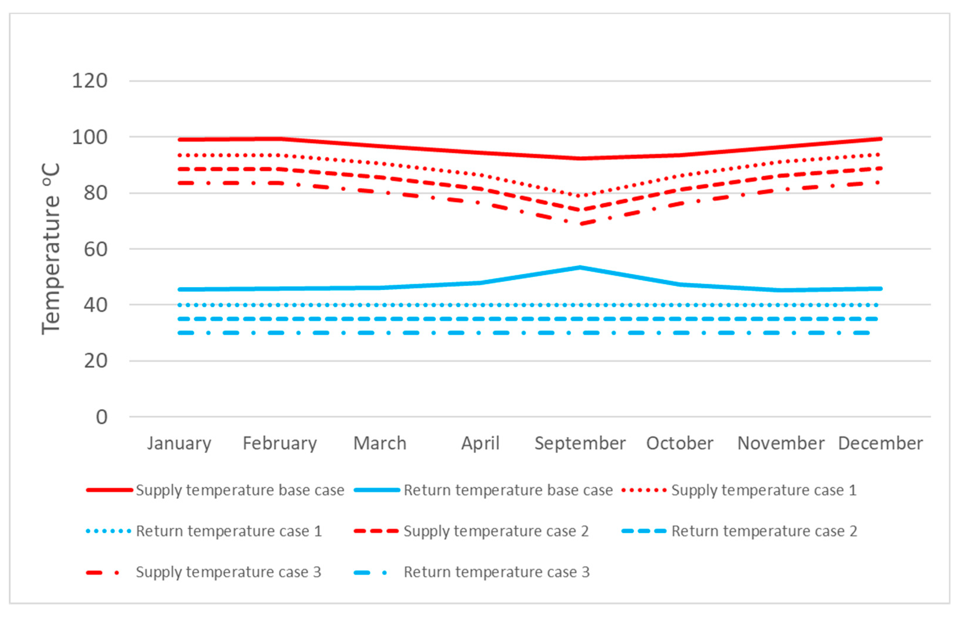
5.1. Temperatures in the Model
In the MODEST model, the assumption was made that the difference between supply temperature and return temperature is equal to the measured base case, i.e. equal to differences compared to temperature measurements from 2015. Four different cases were examined: first a base case with data from measurements, then three different cases with return temperatures and corresponding supply temperatures. The modelled return temperatures were 40 °C, 35 °C and 30 °C. A summary of modelled cases is presented in
Table 5.
The temperatures derived from measurements are presented in
Figure 7. The temperatures used in the model are presented in
Figure 8. The period of May–August was considered to be outside of the heating season, so this period did not have any temperature adjustments.
A small part of the district heating load in today’s system needs a 90 °C supply temperature, so this was the lowest measured temperature during 2015. In this study, that temperature limit was omitted, as this part of the heat load can be supplied with an alternative solution, and is in fact not an absolute obstacle for lower supply temperatures for the rest of the DHS.
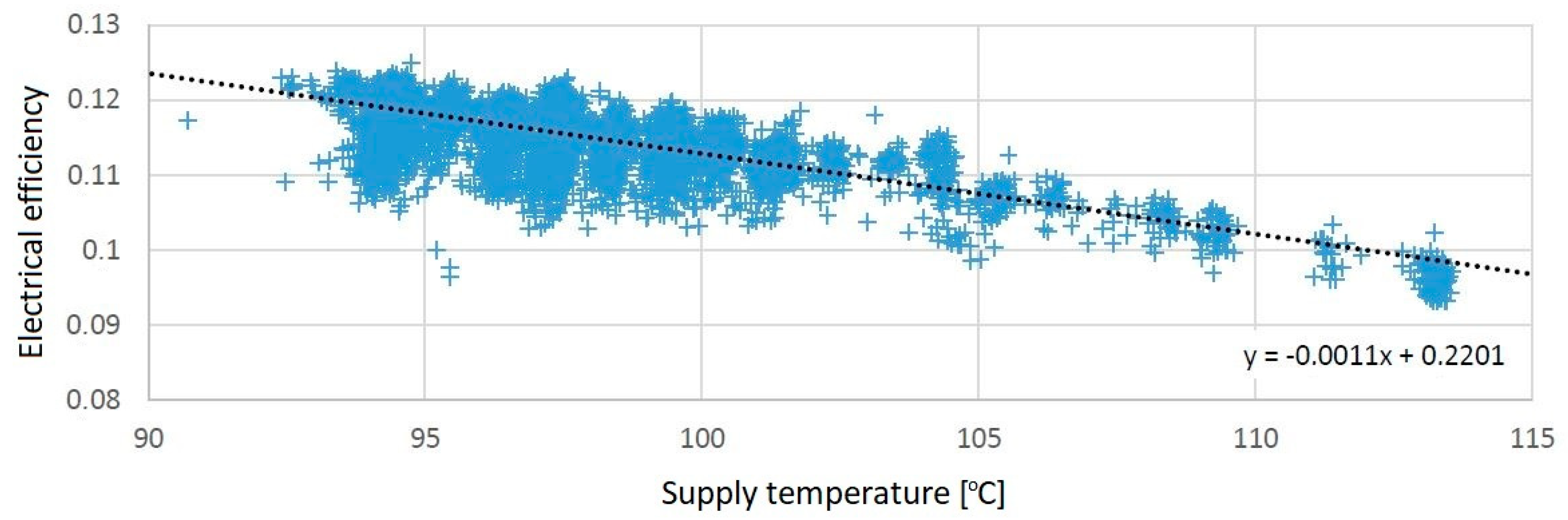
5.2. Efficiencies in the Model
The efficiencies for backpressure turbines and flue gas condensers have been modelled with linear equations for each component. The linear equations have been calculated from plant measurements covering a period of several years. The measurements from a turbine can be seen in
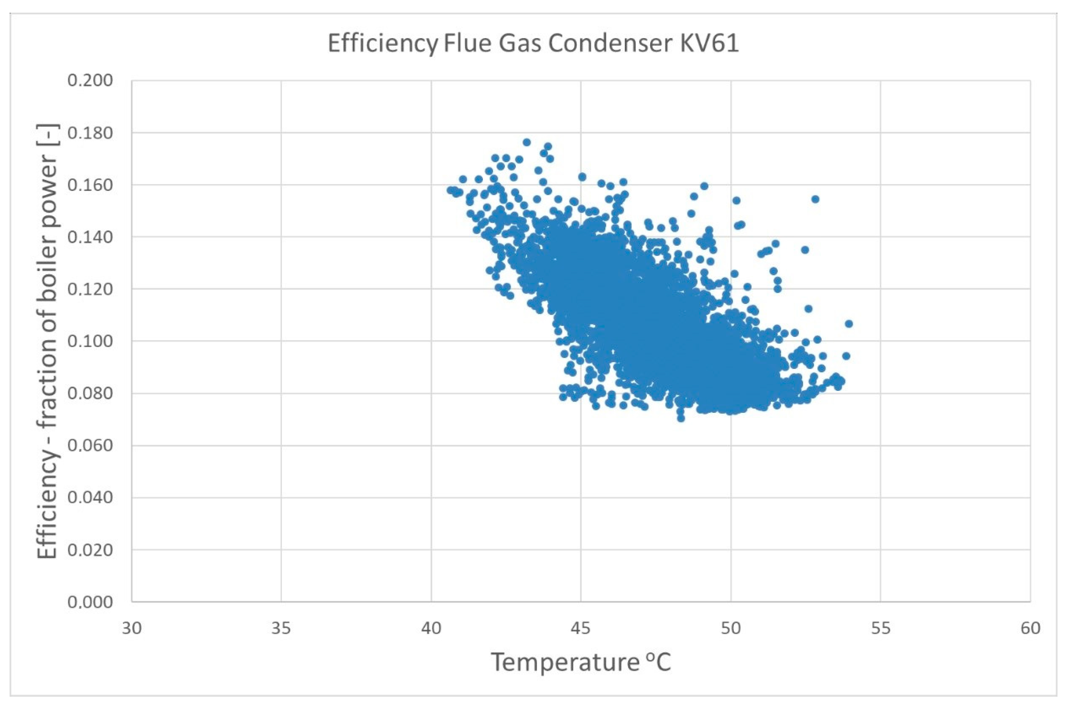
Figure 9, and the measurements from a flue gas condenser in
Figure 10, and the equations for all of the temperature-dependent components can be seen in
Table 6. Looking at these measured efficiencies, it is obvious that they are not ideally linear. However, the most important aspect for this study is the temperature-dependent trend, which is clear for both electrical efficiencies and flue gas condenser efficiencies. A flue gas condenser extracts latent heat from the flue gas to the return water. A greater difference between the flue gas temperature and the return water temperature will increase the amount of extracted heat. For the flue gas condenser (FGC) in
Figure 10, it is very clear that the lower limit for the measured efficiency has a strong correlation with temperature (i.e., a low return temperature is clearly beneficial to FGC efficiency).
5.3. Emissions in the Model
The emission values in
Table 7 are derived from The Environmental Fact Book [
22]. Coal condensing power (CCP) was used as the marginal production unit in the European electricity market, and the turbine efficiency for these plants was considered to be 40%. To evaluate the impact of the saved fuel, the assumption was made that the saved fuel is used in CCP to replace the coal (see, for example, [
23,
24].
6. Model Results
In this section, the results from the Linköping Municipality case study are presented in three different categories—efficiency, GHG emissions, and economic assessment. In
Section 6.1,
Section 6.2 and
Section 6.3, the results are presented as relative values in comparison with the modelled base case in
Figure 11 and
Figure 12.
Table 8 presents the absolute numbers for production and fuel use. The base case and the measured production from 2015 differ regarding the amount for each specific fuel. This is natural because the optimization model “chooses” the fuel and the power plants in a more simplistic way than the real power plant operators do. FGC KV1—Wood and FGC KV50 have not been operated at full power during 2015. However, in the modelled cases, all of the FGCs are assumed to be fully available.
6.1. Efficiencies and Fuel Consumption
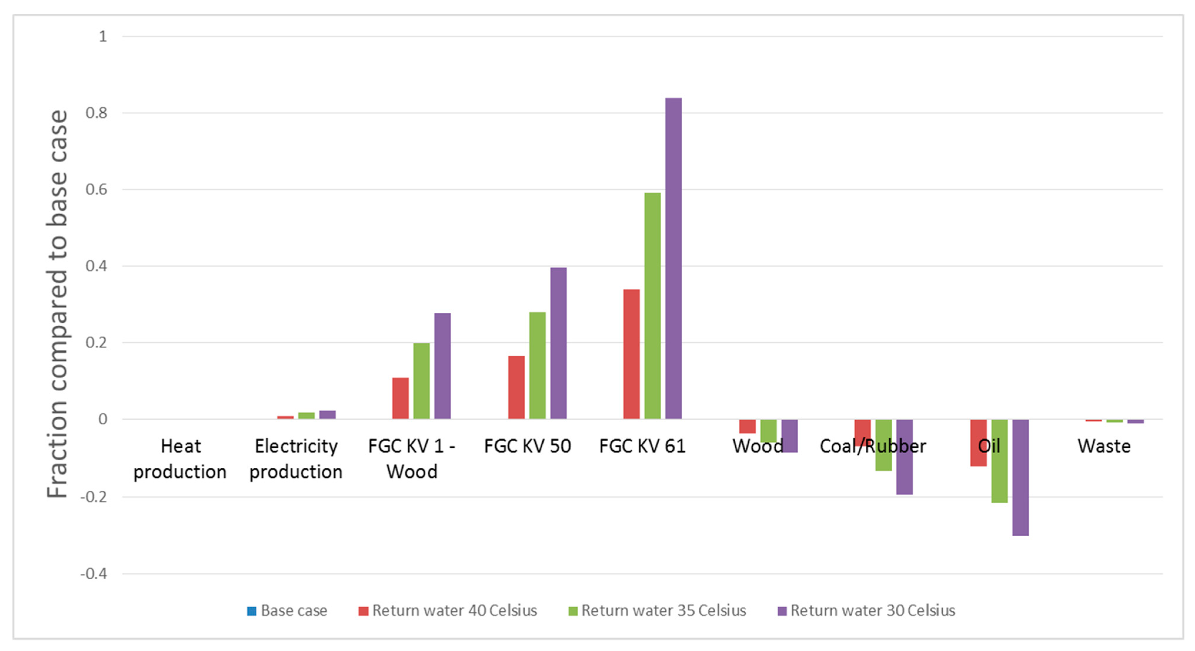
Heat production is a boundary condition in the model, so naturally, this will not differ between the base case and the three cases with controlled return water temperature. For fuel consumption, waste fuel is almost unchanged for all of the cases. This is natural, because it is a preferred fuel in the fuel merit order. Oil use has the largest reduction, with 30% for Case 3. FGC heat is almost doubled, with an 84% increase for KV61 corresponding to 35 GWh of free heat, which, in the base case, is lost with the flue gas. For Case 3, the total increase in FGC heat is 103 GWh, corresponding to around 7% of the total DHS heat.
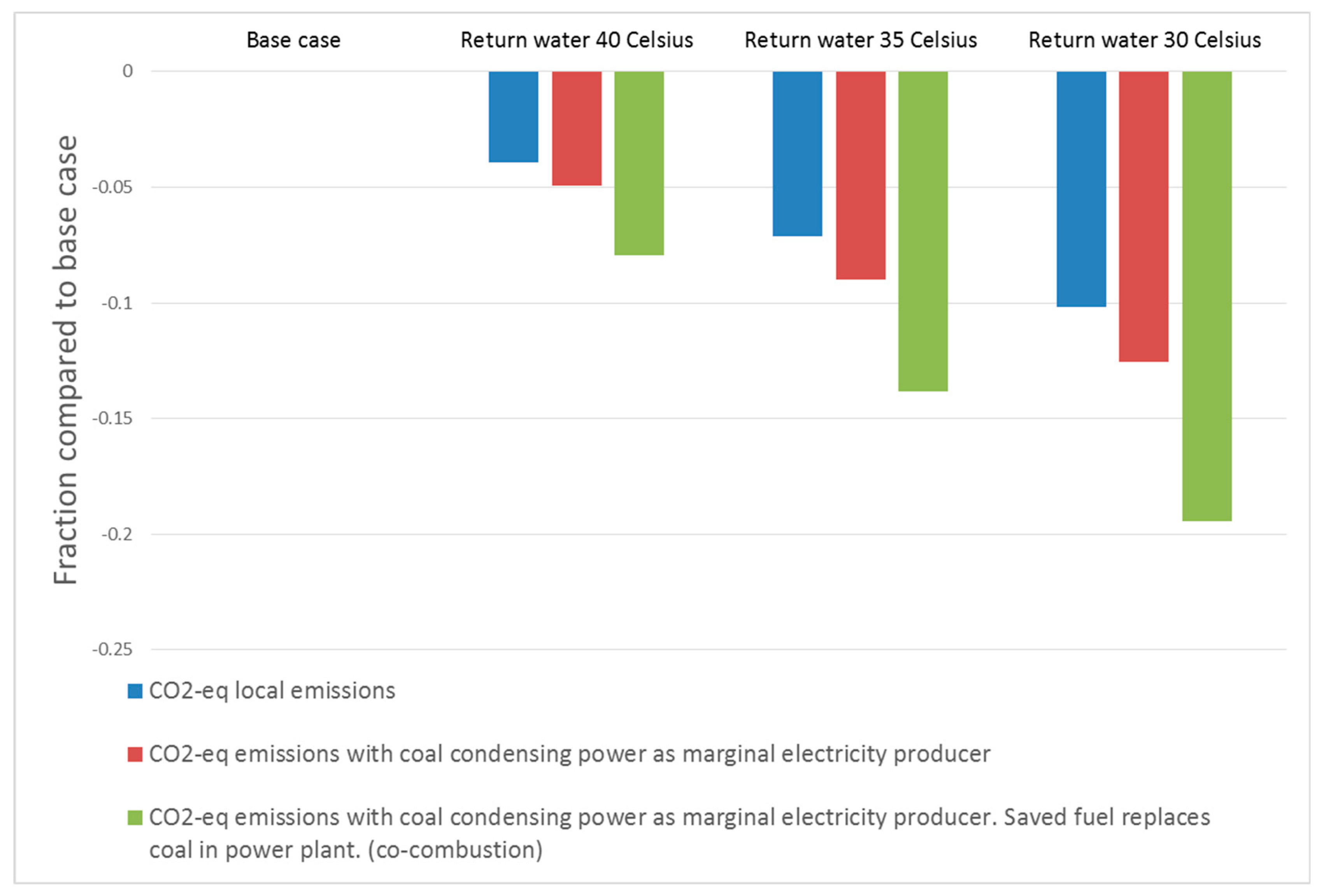
6.2. GHG Emissions
In this study, three different sets of emission data are presented. In an effort to include the market effects caused by the change in local electricity production for the studied DHS, marginal electricity production and marginal fuel consumption are added in evaluation methods 2 and 3. Method 2 only includes market effects in the electricity market, while method 3 includes both the electricity market and the fuel market. In this article, the authors chose to present coal condensing power as the marginal electricity producer, in order to show two ways in which increased electricity production can be valued. To account for only local emissions is one way, giving no value to changes in electricity production. To account for avoided emissions from the most polluting source, coal condensing power, is another way. Olkkonen et al. [
25] present calculations regarding the marginal electricity production for the Finnish, Nordic, and European energy systems, up until 2030. Their calculations indicate that during the winter season, coal condensing power has the largest share between the different marginal generation technologies.
Local emissions.
Emissions with the assumption that coal condensing power is the marginal electricity producer in the European electricity market.
Emissions with the assumption that coal condensing power is the marginal electricity producer in the European electricity market and the assumption that saved fuel replaces coal in the fuel market (co-combustion).
Changes in GHG emissions for the three different evaluation methods are almost linear with the return water temperature. This is a natural consequence of the underlying linear equation for FGC and turbine efficiencies in the model. The temperature trend is clear for all of the cases, but the choice of evaluation method has a strong impact on the absolute emission values. Case 3, evaluated with the third emission evaluation category, showed a reduction of almost 20% in GHG emissions.
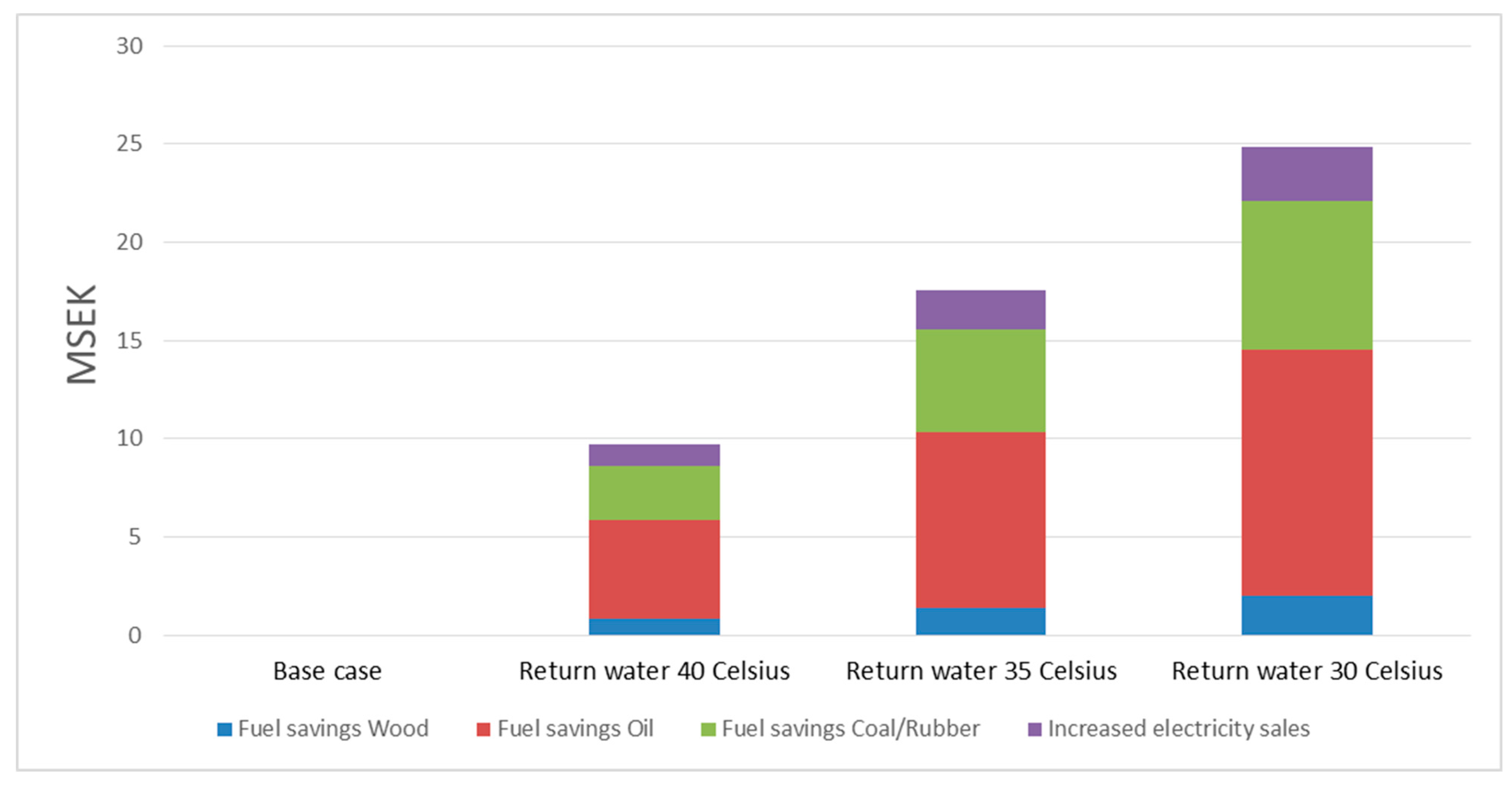
6.3. System Costs Assessment
Higher FGC and turbine efficiencies give savings and higher earnings in accordance with
Figure 13. Oil savings have the largest share, with about 50% of the total economic benefit. Case 3 showed an economic potential of SEK 25 million in yearly improvement; in comparison, it can be mentioned that fuel costs for 2015 were 105 SEK million.
In the figure above, an economic assessment is carried out using the marginal costs and earnings from
Table 9.
7. Discussion
7.1. Static Benefits
As the shortest time for the model time step used in this case study was 48 hours, the quantified results from this model can be considered static or at least quasi static. The static benefits are mainly derived from the alteration of the temperature working point for power plant components and the resulting efficiency improvements. The Linköping DHS has a 20,000 m3 heat storage tank on the supply side, which means that all of the fast load transients can be handled without changing power from the individual production units. In practice, this means that power plants can be operated with only a slow increase or decrease in power, and it also means that a model with long time steps can be a fairly good representation of the DHS.
The quantified results in
Section 6 are all calculated in this quasi static timescale. There are also benefits in the shorter timeframe, but these benefits are highly dependent on the type of technical implementation that is used, and are therefore not quantified in this study. A general description of these benefits follows in the next section.
7.2. Dynamic Benefits
Dynamic benefits for the power plant can be regarded as the benefits in the timespan of 0 to 48 hours (i.e., shorter than the shortest time step in the model). Depending on how an implementation of low-grade heat customers would be carried out, the dynamic properties of the DHS would be different. Compared to today’s system, where the power plant control is limited to the supply side heat storage, many benefits can be identified. These benefits are not included in the quantified benefits represented in
Section 6.
An opportunity to use domestic integrated storage tanks as a buffer would make it easier to plan the power plant production. A demand side management (DSM) solution on the network return side would give the power plant the ability to react to the heat demand fluctuations in the network, instead of trying to forecast loads 4–6 h in advance. With process control terminology, this would mean feedback control instead of open loop control with weather forecasts.
With better process control and a larger heat buffer, a likely system impact is economic savings, because of the fewer starts and stops of individual power plants.
Higher electrical efficiency in the base load situation would give a wider control span in the choice between electricity production and heat production. This applies for both fast and slow transients.
A low-grade heat customer situated downstream from a malfunctioning district heating substation (bad cooling) can reduce the negative impact of the malfunction on the DHS.
7.3. Evaluation of GHG Emissions
The fuel mix for one particular CHP plant or one particular region is not the main issue when considering how markets are linked to each other in the global economy. There is not enough biomass on the planet to sustain our current use of energy [
1], so if all efficiencies and demands remain at the same level, this implies that a fuel switch for one power plant will lead to a fuel switch in the other direction somewhere else. This is the fundamental conclusion to be drawn if we consider the resource limitations of our planet. In a fully connected and closed system, all emissions matter and all efficiencies matter.
To assess the global effects of the proposed action, electricity market connections alone are not enough—some system effects must also reach the fuel market. Here, we use the assumption that fuel that is saved because of higher efficiencies is instead used in co-combustion in CCP plants [
23,
24].
Considering ideal market connections for both the fuel and electricity markets, it is just as harmful to be inefficient with wood as with coal, because inefficiencies in one part of the system play out as higher marginal production for the entire system. In this article, we use coal condensing power as an estimate of that marginal production.
The need for a system perspective is crucial. Looking at this case study, the fuel efficiency gain is around 7% for the 30 °C case, corresponding to 10% lower local GHG emissions, but that number is doubled to almost 20% if electricity market and fuel market connections are considered.
These idealized connections in the electricity market and the fuel market represent a somewhat simplistic view of the European energy system, but we argue that these connections are needed in order to make a fair evaluation of how efficiency gains should be valued.
Looking even further away from the studied object, there is also a possibility of rebound effects in connected markets, in technical systems, or in the form of lifestyle changes (see, for example, [
26]). The rebound effect is omitted in this study, mainly because of complexity.
7.4. System Cost Assessment and Life Cycle Assessment
Model predictions from
Section 6.3 point to a yearly value of SEK 25 million for case 3, with a 30 °C return water temperature. The associated cost for reaching that potential must be considered unknown in this study, where a concrete technical implementation is not stated.
With an unknown construction cost, it is obvious that it becomes hard to promote investments. However, as a hedge against higher fuel costs, the active management of heat customers could be an interesting option to increase network efficiency.
It must also be stated that there is a fundamental contradiction between a free fuel (waste incineration) and investments in efficiency improvements.
A life cycle assessment (LCA) would be beneficial in terms of assessing the impact of these proposed new low-grade heat customers in the DH network. This is important for the evaluation of the proposed action, but remains outside the scope of this case study. It is important to note that there is a considerable difference in environmental impact between, for example, the reuse of radiators, adjustment of working points for valves, or installation of newly produced heating substations. With the active management of heat customers, both LCA and DHS efficiency can be included in future network development.
7.5. DHS Development
Looking at Linköping Municipality in 2050, with an efficient energy system that mitigates the problem of GHG emissions in an effective manner, it seems unlikely that the existing DHS will not be a part of that system. However, the authors also believe that it is unlikely that the supply and return temperatures in the DH network will remain at today’s levels, when the benefits of lower temperatures are clear and technologies are available.
The assessment and evaluation of GHG emissions is crucial for understanding and interpreting how different technologies contribute to an increase or decrease in GHG emissions. A system approach gives a wider view, but also adds numerical uncertainties and increases the number of assumptions. Given that the effect of GHG emissions is a global issue, this leads us to the conclusion that the system approach is favourable.
A less detailed approach and focus on the trends and the wider system perspective show us that some observations can be made. DH is a well-established technology, and the need for heating will—with high degree of certainty—remain, even in a future low energy society, in 2050. With a system control perspective, it is possible to improve the situation for the CHP plant with existing technology. Lower return water temperature is beneficial for DHS efficiency, and the function is continuous regarding temperature. The continuous function means that an experimental introduction of low-grade heat customers can be initiated and then evaluated in an iterative process.
With the results from this case study, we propose that an interesting next move for DHS with CHP would be to introduce low-grade heat customers on the DH return water pipes, to achieve better system control and higher system efficiency.
During 2016, TvAB commissioned another waste incineration plant with a production capacity of 83 MW and an electrical efficiency of 22.5%. In practice, this means that the economic benefits of lower return temperature are greatly reduced for TvAB. However, considering electricity market connections and fuel market connections, the potential for GHG emission reduction, with the actions proposed in this paper, still remains.
8. Conclusions
The active management of customers in a DHS can lower return water temperatures faster and in the long run lead to better controlled return water temperatures. Active management is defined as an adjustment of a domestic heating system in order to improve DHS efficiency without affecting the heating service for the individual building.
In this study, the effects of introducing active management within a local DHS in Linköping, Sweden, have been analysed.
The conclusions from the study are the following:
Possible efficiency gains of around 7%, corresponding to 103 GWh heat
GHG emission reduction of 4–20%
Reduced system cost by SEK 25 million per year
The authors believe that the examined system shows results that are generalizable to other Swedish DHSs, given the high degree of technical similarity between these systems. However, individual differences between DHSs regarding fuel mixture and electrical efficiency for turbines must be acknowledged.
Author Contributions
All the parts of the manuscript were discussed among the two authors. T.R. was the main author and wrote all the parts.
Funding
This research received no external funding.
Acknowledgments
The work has been carried out under the auspices of Fjärrsyn (district heating and cooling research programme) and the Swedish District Heating Association. We are grateful to the people at Tekniska verken AB who gave us measurements and data, especially Joakim Holm, who supplied a great deal of valuable information. We also wish to thank our supporting research group, namely: Lina La Fleur, student, Linköping University; Stefan Blomquist, student, Linköping University; Tina Lidberg, student, University of Gävle (HiG); Mattias Gustafsson, student, University of Gävle; and Rasmus Lund, University of Copenhagen.
Conflicts of Interest
The authors declare no conflict of interest.
References
- Moriarty, P.; Honnery, D. What is the global potential for renewable energy? Renew. Sustain. Energy Rev. 2012, 16, 244–252. [Google Scholar] [CrossRef]
- Haberl, H.; Erb, K.H.; Krausmann, F.; Bondeau, A.; Lauk, C.; Müller, C.; Plutzar, C.; Steinberger, J.K. Global bioenergy potentials from agricultural land in 2050: Sensitivity to climate change, diets and yields. Biomass Bioenergy 2011, 35, 4753–4769. [Google Scholar] [CrossRef] [PubMed]
- de Castro, C.; Mediavilla, M.; Miguel, L.J.; Frechoso, F. Global solar electric potential: A review of their technical and sustainable limits. Renew. Sustain. Energy Rev. 2013, 28, 824–835. [Google Scholar] [CrossRef]
- Hoes, O.A.C.; Meijer, L.J.J.; van der Ent, R.J.; van de Giesen, N.C. Systematic high-resolution assessment of global hydropower potential. PLoS ONE 2017. [Google Scholar] [CrossRef] [PubMed]
- Energimyndigheten. Energiläget 2015. Available online: http://www.energimyndigheten.se (accessed on 4 May 2018).
- Lund, H.; Werner, S.; Wiltshire, R.; Svendsen, S.; Thorsen, J.E.; Hvelplund, F.; Mathiesenf, B.V. 4th Generation District Heating (4GDH): Integrating smart thermal grids into future sustainable energy systems. Energy 2014, 68, 1–11. [Google Scholar] [CrossRef]
- Dagilis, V.; Vaitkus, L.; Balčius, A.; Gudzinskas, J.; Lukoševičiu, V.S. Low Grade Heat Recovery System For Woodfuel Cogeneration Plant Using Water Vapour Regeneration. Thermal Sci. 2018, 22, 2667–2677. [Google Scholar] [CrossRef]
- Ziviani, D.; Suman, A.; Lecompte, S.; de Paepe, M.; van den Broek, M.; Spina, P.R.; Pinelli, M.; Venturini, M.; Beyene, A. Comparison of a Single-screw and a Scroll Expander under Part-load Conditions for Low-grade Heat Recovery ORC Systems. Energy Procedia 2014, 61, 117–120. [Google Scholar] [CrossRef]
- Lundström, L.; Wallin, F. Heat demand profiles of energy conservation measures in buildings and their impact on a district heating system. Appl. Energy 2016, 161, 290–299. [Google Scholar] [CrossRef]
- Harrestrup, M.; Svendsen, S. Changes in heat load profile of typical Danish multi-storey buildings when energy-renovated and supplied with low-temperature district heating. Int. J. Sustain. Energy 2015, 34, 232–247. [Google Scholar] [CrossRef]
- SvenskFjärrvärme. 2016. Available online: http://www.svenskfjarrvarme.se/Statistik--Pris/Fjarrvarme/Leveranser/ (accessed on 4 June 2018).
- Zhang, L.; Gudmundsson, O.; Thorsen, J.; Li, H.; Li, X.; Svendsen, S. Method for reducing excess heat supply experienced in typical Chinese district heating systems by achieving hydraulic balance and improving indoor air temperature control at the building level. Energy 2016, 107, 431–442. [Google Scholar] [CrossRef]
- Tunzi, M.; Skaarup, D.; Østergaard; Svendsen, S.; Boukhanouf, R.; Cooper, E. Method to investigate and plan the application of low temperature district heating to existing hydraulic radiator systems in existing buildings. Energy 2016, 113, 413–421. [Google Scholar] [CrossRef]
- Yang, X.; Li, H.; Svendsen, S. Decentralized substations for low-temperature district heating with no Legionella risk, and low return temperatures. Energy 2016, 110, 65–74. [Google Scholar] [CrossRef]
- Hoes, P.; Hensen, J.L.M. The potential of lightweight low-energy houses with hybrid adaptable thermal storage: Comparing the performance of promising concepts. Energy Build. 2016, 110, 79–93. [Google Scholar] [CrossRef]
- Churchman, C.W. The Systems Approach; A Delta book; Dell Publishing Co.: New York, NY, USA, 1968. [Google Scholar]
- Kensby, J.; Trüschel, A.; Dalenbäck, J.-O. Potential of residential buildings as thermal energy storage in district heating systems – Results from a pilot test. Appl. Energy 2015, 137, 773–781. [Google Scholar] [CrossRef]
- Fredrik Wernstedt, C.J. SvenskFjärrvärme 2009. Demostrationsprojekt Inom Effekt Och Laststyrning. 2009. Available online: http://www.fukt.bsnet.se/~uncle/papers/effektstyrning.pdf (accessed on 15 May 2019).
- Henning, D. Optimisation of Local and National Energy Systems: Development and Use of the MODEST Model; Linköping Studies in Science and Technology: Linköping, Sweden, 1999. [Google Scholar]
- Lidberg, T.; Olofsson, T.; Trygg, L. System impact of energy efficient building refurbishment within a district heated region. Energy 2016, 106, 45–53. [Google Scholar] [CrossRef]
- Gebremedhin, A. Introducing District Heating in a Norwegian town – Potential for reduced Local and Global Emissions. Appl. Energy 2012, 95, 300–304. [Google Scholar] [CrossRef]
- Gode, J.M.F.; Hagberg, L.; Palm, D. Värmeforsk 2011. Miljöfaktaboken 2011. Estimated emission factors for fuels, electricity, heat and transport in Sweden. 2011. Available online: https://energiforskmedia.blob.core.windows.net/media/17907/miljoefaktaboken-2011-vaermeforskrapport-1183.pdf (accessed on 15 May 2019).
- Judl, J.; Koskela, S.; Korpela, T.; Karvosenoja, N.; Häyrinen, A.; Rantsi, J. Net environmental impacts of low-share wood pellet co-combustion in an existing coal-fired CHP (combined heat and power) production in Helsinki, Finland. Energy 2014, 77, 844–851. [Google Scholar] [CrossRef]
- Sahu, S.G.; Chakraborty, N.; Sarkar, P. Coal–biomass co-combustion: An overview. Renew. Sustain. Energy Rev. 2014, 39, 575–586. [Google Scholar] [CrossRef]
- Olkkonen, V.; Syri, S. Spatial and temporal variations of marginal electricity generation: The case of the Finnish, Nordic, and European energy systems up to 2030. J. Clean. Prod. 2016, 126, 515–525. [Google Scholar] [CrossRef]
- Olsson, A.; Grönkvist, S.; Lind, M.; Yan, J. The elephant in the room—A comparative study of uncertainties in carbon offsets. Environ. Sci. Policy 2016, 56, 32–38. [Google Scholar] [CrossRef]
Figure 1.
Supplied district heating in Sweden. The growth period for the district heating market is coming to an end and is moving into a period of maintenance. [
2].
Figure 1.
Supplied district heating in Sweden. The growth period for the district heating market is coming to an end and is moving into a period of maintenance. [
2].
Figure 2.
Illustration of a traditional district heating system: (1) Combined heat and power (CHP) power plants; (2) traditional heat load—district heat (DH) substations in parallel; (3) studied system with boundary connections to the fuel and electricity market.
Figure 2.
Illustration of a traditional district heating system: (1) Combined heat and power (CHP) power plants; (2) traditional heat load—district heat (DH) substations in parallel; (3) studied system with boundary connections to the fuel and electricity market.
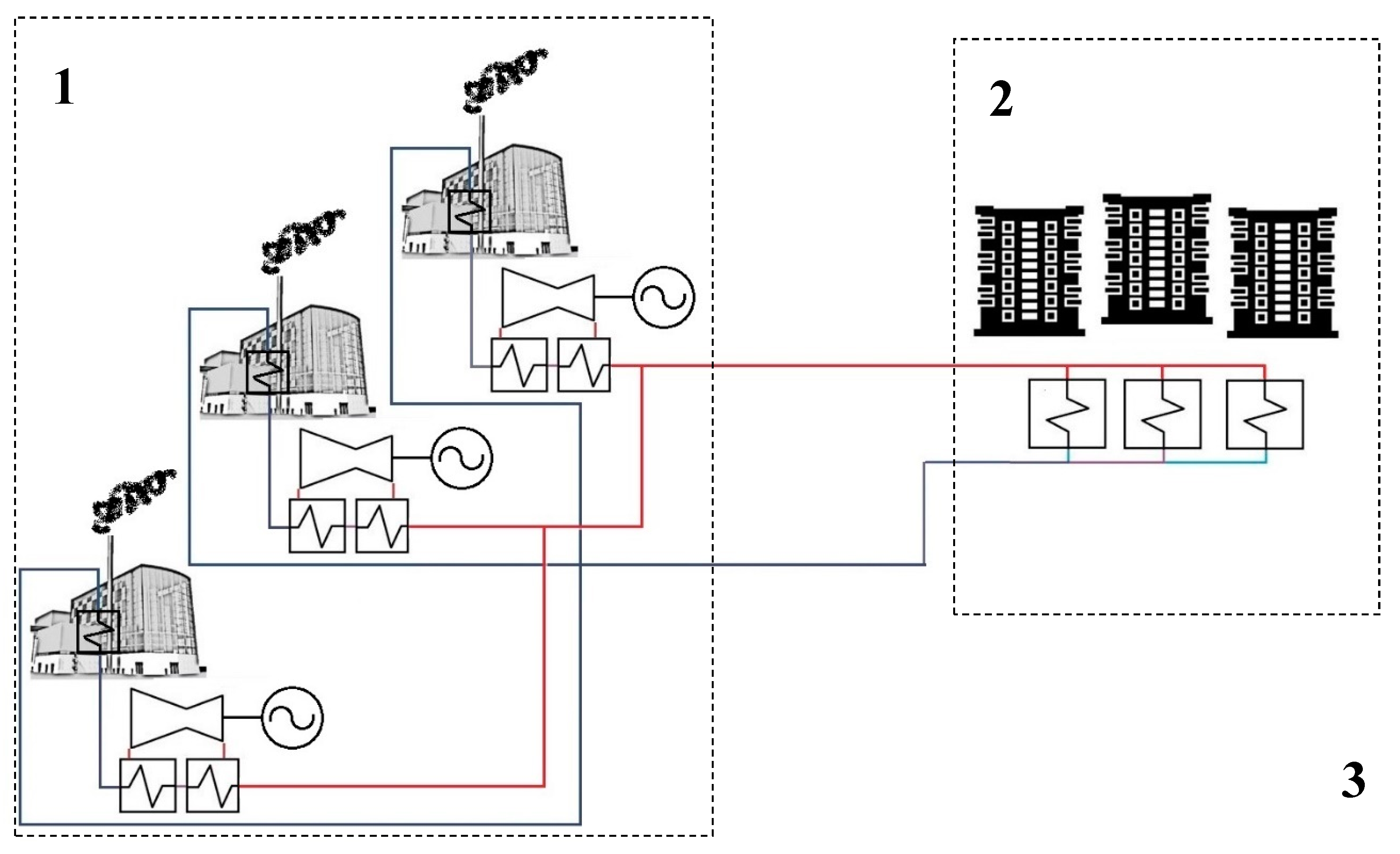
Figure 3.
Illustration of a district heating system with controllable low-grade heat customers: (1) CHP power plants; (2) traditional heat load—DH substations in parallel; (3) low-grade heat customers; (4) temperature-dependent flue gas condenser (FGC); (5) temperature-dependent steam turbine; (6) studied system with boundary connections to fuel and electricity market.
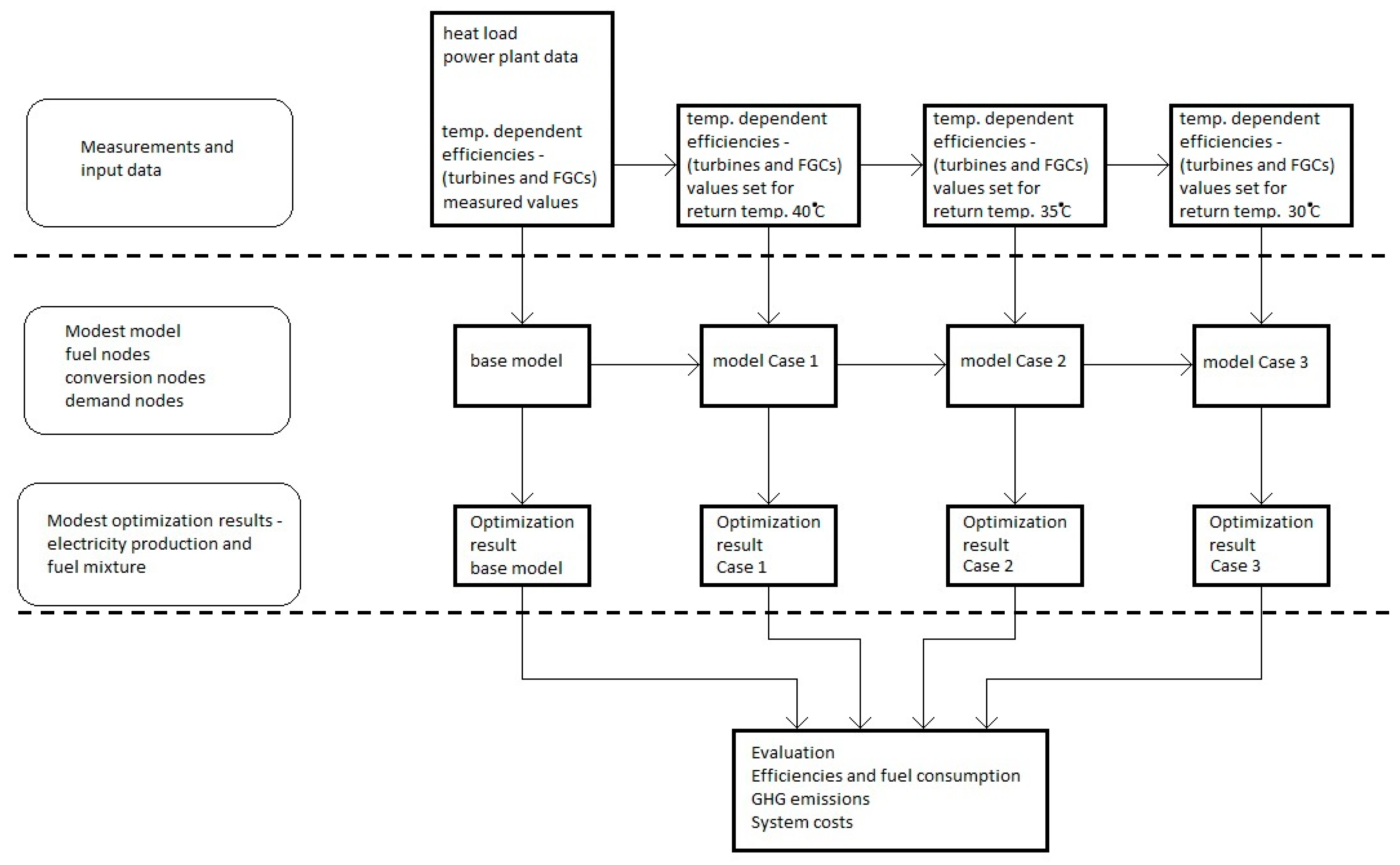
Figure 4.
Schematic illustration of the workflow for the study. Horizontal lines show borders for the Model for Optimization of Dynamic Energy Systems with Time-dependent components and boundary conditions (MODEST) model.
Figure 4.
Schematic illustration of the workflow for the study. Horizontal lines show borders for the Model for Optimization of Dynamic Energy Systems with Time-dependent components and boundary conditions (MODEST) model.
Figure 5.
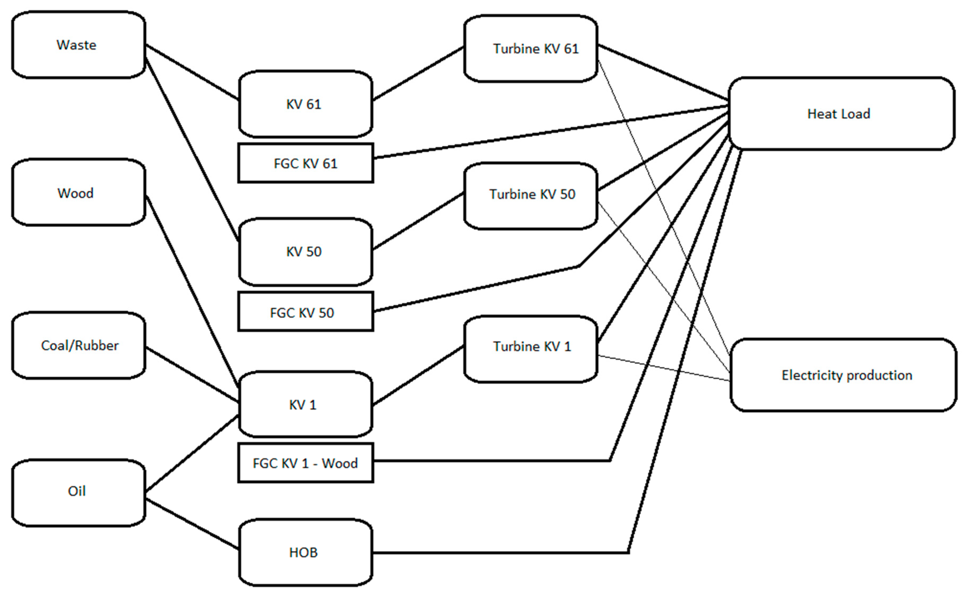
Illustration of nodes and flows in the model.
Figure 5.
Illustration of nodes and flows in the model.
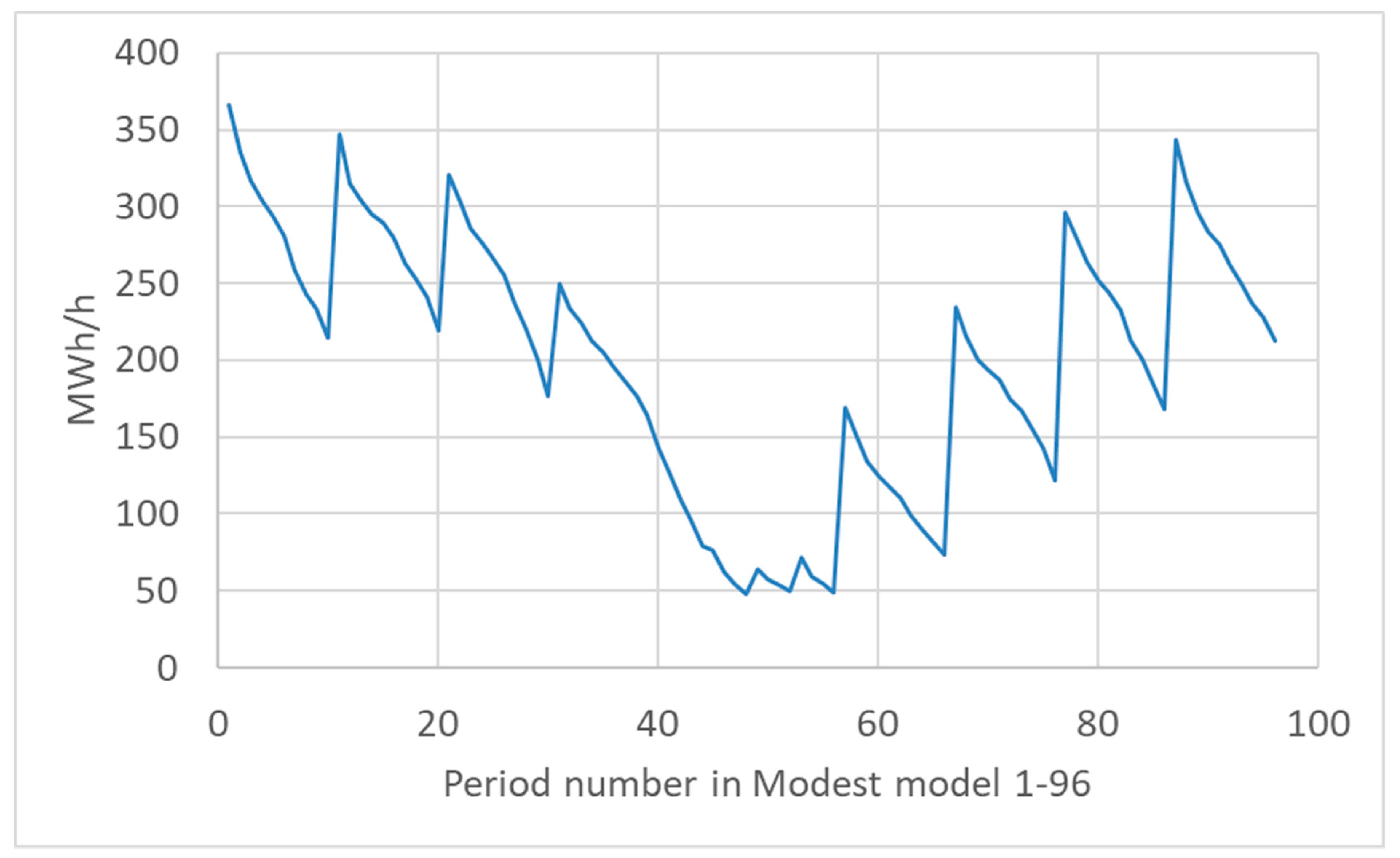
Figure 6.
Heat load in the model, presented with monthly duration diagram (i.e., days sorted by heat load in each month). For days with higher heat loads are modelled in greater detail, see
Table 4.
Figure 6.
Heat load in the model, presented with monthly duration diagram (i.e., days sorted by heat load in each month). For days with higher heat loads are modelled in greater detail, see
Table 4.
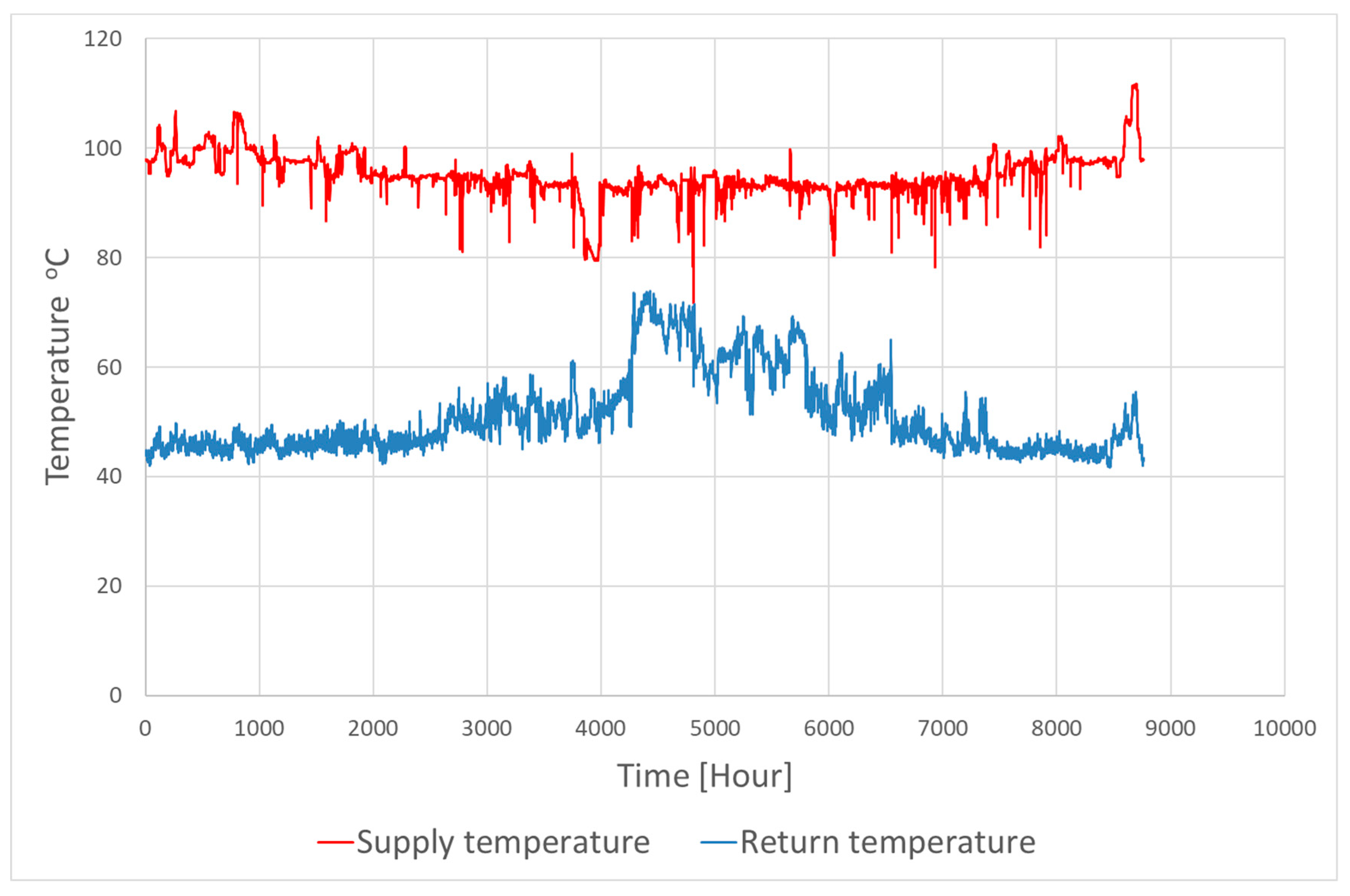
Figure 7.
Measured supply and return temperatures in Linköping’s DHS in 2015.
Figure 7.
Measured supply and return temperatures in Linköping’s DHS in 2015.
Figure 8.
System temperatures in the MODEST model.
Figure 8.
System temperatures in the MODEST model.
Figure 9.
Measured efficiencies for KV50 turbine—waste incineration plant.
Figure 9.
Measured efficiencies for KV50 turbine—waste incineration plant.
Figure 10.
Flue gas condenser efficiency for KV 61 waste incineration unit. Samples are collected during several years and during different operation modes. There are variations in boiler power, fuel moisture, outdoor pressure, and so on. This gives a great data dispersion, but the temperature trend is clear.
Figure 11.
Modelled changes in whole year efficiencies and fuel consumption.
Figure 11.
Modelled changes in whole year efficiencies and fuel consumption.
Figure 12.
Modelled changes in GHG emissions for the examined cases with three different system boundaries.
Figure 12.
Modelled changes in GHG emissions for the examined cases with three different system boundaries.
Figure 13.
Economic figures for model results, 2015. Costs and earnings from
Table 9.
Figure 13.
Economic figures for model results, 2015. Costs and earnings from
Table 9.
Table 1.
Production units in Linköping’s district heating system. FGC—flue gas condenser.
Table 1.
Production units in Linköping’s district heating system. FGC—flue gas condenser.
| Power Plant | Maximum Output (MW Thermal Power) | Fuel | Flue Gas Condenser Efficiency (% of Boiler Power) | Steam Turbine Efficiency (Electricity Production/Input Heat) |
|---|
| KV 50 | 72 | Waste incineration | 15–40 | 0.10–0.15 |
| KV 61 | 66 | Waste incineration | 0–22 | 0.17–0.27 |
| KV 1—wood | 60 | Wood | 20–40 | 0.18–0.26 |
| KV 1—coal | 60 | Coal/rubber | FGC not available | 0.18–0.26 |
| KV 1—oil | 120 | Oil | FGC not available | 0.18–0.26 |
| HOBs (Heat only boilers, several distributed in DH network) | 240 | Oil | FGC not available | No turbine |
Table 2.
Details of the Model for Optimization of Dynamic Energy Systems with Time-dependent components and boundary conditions (MODEST) model. DHS—district heating system.
Table 2.
Details of the Model for Optimization of Dynamic Energy Systems with Time-dependent components and boundary conditions (MODEST) model. DHS—district heating system.
| Variable | Linköping DHS | MODEST Model Linköping DHS |
|---|
| Temperature in supply flow and return flow | Supply: Measured on an hourly basis
Return: Measured on an hourly basis | Represented in the model by a function that affects efficiency in turbines and flue gas condensers for each time step |
| Heat load | Measured daily in 2015 | From 2015 measurements—monthly duration |
| Heat losses in distribution pipes | Not measured and not calculated | Not included |
| Heat losses in flue gas | Not measured and not calculated | Included indirectly via FGC efficiency |
| Flue gas condenser efficiencies | Efficiencies measured with historic values from 2010–2012 | Included in model with linear equation |
| Electricity use for distribution pumps | Measured value:
4391 MWh (0.3% of heat load) | Not included |
| Turbine efficiencies | Efficiencies measured with historic values from 2010–2012 | Included in model with linear equation |
| Supply temperature management | Active management can choose between electricity production and heat production | Not included in model as a result of the monthly duration heat load input. Supply temperature in fixed relation to return temperature |
Table 3.
Fuel prices in the model. CHP—combined heat and power.
Table 3.
Fuel prices in the model. CHP—combined heat and power.
| Fuel | Price in Model |
|---|
| Waste | 0 SEK/MWh |
| Wood | 70 SEK/MWh |
| Coal/rubber | 180 SEK/MWh |
| Oil CHP | 320 SEK/MWh |
| Oil HOB | 600 SEK/MWh |
Table 4.
Time division in the model.
Table 4.
Time division in the model.
| Period | Time Resolution |
|---|
| January–April (first 10 days in monthly duration diagram) | Average heat load for 48 h periods |
| January–April (remaining days in monthly duration diagram) | Average heat load for 96 h periods |
| May–August | Average heat load for each week |
| September–December (first 10 days in monthly duration diagram) | Average heat load for 48 h periods |
| September–December (remaining days in monthly duration diagram) | Average heat load for 96 h periods |
Table 5.
Description of the studied cases.
Table 5.
Description of the studied cases.
| Case | Description |
|---|
| Base case | Efficiencies for turbines and FGC corresponding to temperature measurements from 2015. |
| Case 1 | Low-grade heat customers with sufficient heat load to control return water temperature to 40 °C. |
| Case 2 | Low-grade heat customers with sufficient heat load to control return water temperature to 35 °C. |
| Case 3 | Low-grade heat customers with sufficient heat load to control return water temperature to 30 °C. |
Table 6.
Temperature-dependent efficiencies in the MODEST model (Y = efficiency as fraction of boiler power; X = temperature [°C]).
Table 6.
Temperature-dependent efficiencies in the MODEST model (Y = efficiency as fraction of boiler power; X = temperature [°C]).
| Power Plant Component | Efficiency Equation, Fraction of Boiler Power |
|---|
| Turbine KV 1 ** | Y = −0.0015·X + 0.3907 |
| Turbine KV 50 | Y = −0.0011·X + 0.2201 |
| Turbine KV 61 | Y = −0.0019·X + 0.3938 |
| Flue gas condenser KV 1 – wood | Y = −0.0064·X + 0.5557 |
| Flue gas condenser KV 50 – waste | Y = −0.0069·X + 0.54 |
| Flue gas condenser KV 61 – waste | Y = −0.0061·X + 0.394 |
Table 7.
Emissions of greenhouse gas (GHG) CO
2-eq for each fuel, The Environmental Fact Book [
22].
Table 7.
Emissions of greenhouse gas (GHG) CO
2-eq for each fuel, The Environmental Fact Book [
22].
| Fuel | Emissions kg CO2-eq/MWh |
|---|
| Wood | 14 |
| Oil | 288 |
| Coal/rubber | 360 |
| Waste | 136 |
| Coal | 388 |
Table 8.
Model results, production, and fuel use for all cases. The grey field presents measured production from 2015. All numbers in MWh.
Table 8.
Model results, production, and fuel use for all cases. The grey field presents measured production from 2015. All numbers in MWh.
| Case | Heat Production | Electricity Production | FGC KV 1—Wood | FGC KV50 | FGC KV61 | Wood | Coal/Rubber | Oil | Waste |
|---|
| Measured production 2015 | 1,481,617 | 234,069 | 44,118 | 82,717 | 49,501 | 463,585 | 153,991 | 63,411 | 1,205,444 |
| Base case | 1,459,250 | 276,534 | 69,418 | 123,998 | 40,994 | 333,435 | 212,109 | 122,962 | 1,137,138 |
| Case 1 | 1,459,250 | 279,399 | 77,004 | 144,472 | 54,870 | 321,109 | 197,195 | 108,048 | 1,130,845 |
| Case 2 | 1,459,250 | 281,722 | 83,253 | 158,764 | 65,216 | 313,657 | 183,661 | 96,408 | 1,127,948 |
| Case 3 | 1,459,250 | 283,139 | 88,752 | 173,050 | 75,376 | 304,977 | 170,768 | 85,779 | 1,124,693 |
Table 9.
Marginal fuel cost for power plant, real values from 2015, including taxes. Source: TvAB (the local energy company).
Table 9.
Marginal fuel cost for power plant, real values from 2015, including taxes. Source: TvAB (the local energy company).
| Fuel | Electricity | Heat |
|---|
| Waste | 0 SEK/MWh | 0 SEK/MWh |
| Wood | 70 SEK/MWh | 70 SEK/MWh |
| Coal/rubber | 170 SEK/MWh | 187 SEK/MWh |
| Oil | 316 SEK/MWh | 342 SEK/MWh |
© 2019 by the authors. Licensee MDPI, Basel, Switzerland. This article is an open access article distributed under the terms and conditions of the Creative Commons Attribution (CC BY) license (http://creativecommons.org/licenses/by/4.0/).


