Development of Floquet Multiplier Estimator to Determine Nonlinear Oscillatory Behavior in Power System Data Measurement

Abstract

Measurement-based technology has been developed in the area of power transmission systems with phasor measurement units (PMU). Using high-resolution PMU data, the oscillatory behavior of power systems from general electromagnetic oscillations to sub-synchronous resonances can be observed. Studying oscillations in power systems is important to obtain information about the orbital stability of the system. Floquet multipliers calculation is based on a mathematical model to determine the orbital stability of a system with the existence of stable or unstable periodic solutions. In this paper, we have developed a model-free method to estimate Floquet multipliers using time series data. A comparative study between calculated and estimated Floquet multipliers has been performed to validate the proposed method. The results are provided for a sample three-bus power system network and the system integrated with a doubly fed induction generator.

1. Introduction

Over the past few decades, power systems have experienced significant changes regarding the amount of power consumed as well as the complexity of the network. Voltage instabilities tend to occur in power systems that are heavily loaded or in faulty condition. There are various indicators of voltage instability, which are determined by the generator, load dynamics, and network structure [1]. Nonlinear oscillatory behaviors are usually noticeable even before the voltage collapse occurs. These oscillatory behaviors can be observed with high-resolution devices. After detecting nonlinear oscillatory behavior, the type of oscillation needs to be determined to check whether the condition will be harmful to the power system.

Nonlinear oscillatory behaviors are an intrinsic characteristic of power systems caused by the structure of the system under a specific condition. To analyze nonlinear behavior, system topology and dynamics are necessary to describe the system mathematically. Then, mathematical expressions of the system, such as state equations or system Jacobian matrix, can provide detailed information on the current status of the system. In power systems, practical issues such as special nonlinear oscillatory behavior can be revealed by time series data measurements. However, without the input of other measurement data or conditions, it is hard to assess the system state since the information about the system is limited to local measurements. Fortunately, studies related to limited time series data applications have been conducted using mathematical models.

Based on the mathematical modeling of nonlinear system local stability, calculation of the maximal Lyapunov exponent in time series data was proposed by Wolf et al. [2]. Other researchers improved the calculation efficiency of the maximal Lyapunov exponent in time series data [3,4]. The maximal Lyapunov exponent was also modified for applications in time series data on power systems [5,6]. The maximal Lyapunov exponent is a stability index that is strongly connected to the fluctuation of data. If the maximum Lyapunov exponent of the system is negative (positive), then the nearby system trajectories will converge (diverge) toward each other [7]. In the results of [5], the maximal Lyapunov exponent in time series data was reasonable compared to the original signal of the bus voltage after the fault was cleared. In other words, all the simulations in [5] involved increased oscillation or oscillation with large amplitudes of approximately 0.4 p.u. However, in reality, the maximal Lyapunov exponent in time series data is difficult to apply since it strongly depends on the initial values and data size. For example, when the bus voltage oscillates for a long time interval, the maximal Lyapunov exponent will be different for the initial values and data size selected. When oscillation occurs, the maximal Lyapunov exponent also fluctuates, regardless of whether it is positive or negative, which makes it hard to determine system stability. Therefore, the characteristics or stability of the oscillatory behavior of nonlinear systems differ from local stability, especially for time series data. There are some certain approaches (real-time or near-to-real-time) in large amounts of literature to detect local stability such as positively or negatively damped oscillations (for example, Voltage stability indices or maximum Lyapunov exponent [5,6]). However, there are few existing solutions or approaches in power systems or other applicable engineering field to detect uncertain response as marginal stability (mathematically defined but not practically). However, still marginal stability issues such as sustained oscillation or forced oscillation could lead some damages or instability to power system [8]. So, this paper focuses on the feature of periodic stability of the power system dynamics.

Knowing the type of oscillatory behavior is important to predict how the oscillatory behavior of the system will change. In practical applications, filter-based approaches are often used to detect and classify the oscillation [9]. For mathematically based applications, the stability of nonlinear oscillatory behaviors is determined with a Floquet multiplier. A Floquet multiplier is the eigenvalue of a matrix that gives orbital stability for the periodic solution of the system. A solution is stable when all the calculated moduli of the eigenvalues in the monodromy matrix are below the unity. A monodromy matrix is a matrix that influences whether the periodic solution decays or grows for the initial perturbation [7]. In classical texts, a geometric concept called a Poincaré map has been introduced to discuss some behaviors of periodic solutions in terms of a Floquet multiplier [7]. One study [10] introduced a method for nonlinear time series analysis that provided some guidelines on constructing a Poincaré map from data-based signals. However, the method reduced the phase space dimensionality one at a time to turn the continuous time flow into a discrete time map. It notes that the method is the intersection count and not simply proportional to the original time t of the flow. The number of intersections that are counted might be very small, since the parameter is over specific value or interval of unstable region (the chaos), the system may collapse. Therefore, surfaces should be carefully selected or else they will not contain enough information on the signal.

From the perspective of biomechanical engineering, orbital stability is defined using estimated Floquet multipliers from measured data of physical rotation and orbital movement [11,12,13]. The study by [11] provided a method that generated accurate estimates with noisy experimental data. However, there is no generalized method to choose the proper Poincaré section. Moreover, the verification of the estimated Floquet multiplier against the calculated Floquet multiplier in an actual system model is required.

In this paper, the selection of Poincaré sections for time series dimensions is proposed. Then, the Floquet multiplier is estimated for a one-dimensional Poincaré section. The estimation technique is based on linear regression applied not only to a simple three-bus system but a complex mathematical model of a power system with a wind generator modeled as a doubly fed induction generator (DFIG).

The paper starts with an introduction of the stability of a periodic solution. Then, mathematical concepts of the Poincaré section and Floquet multiplier will be expanded to the proposed method. Comparison of the proposed method and calculated Floquet multipliers will be performed in a test power grid that is integrated with DFIG. Three noteworthy summaries are provided followed by the conclusion.

2. Stability of Periodic Solutions

Power grid dynamics with initial values $t_0$ are shown as follows:

$$\begin{array}{c}\hfill \dot{x}=f(t,x),x(t_0)=x_0\end{array}$$

(1)

System stability can be determined by the real value of eigenvalue as system is linear. However, for a nonlinear system, there are plenty of ways to determine system stability. The maximal Lyapunov exponent is an indicator that gives information on stability of time-dependent solution from Equation (1). The fluctuation of solution can be decreased as maximal Lyapunov exponent is negative and vice versa. However, different approaches are required to analyze behavior as the solution is oscillating. A monodromy matrix gives the characteristics of the oscillatory solution of the nonlinear system (1).

2.1. Monodromy Matrix

Stability of periodic solutions in dynamic systems can be represented by using a mathematical tool. Suppose the solution $x^{\ast }$ is a periodic feature of constant frequency f and its period T as time evolves. The problem of instability of periodic solutions have been studied within the framework of the methods developed by [7]. The trajectories of Equation (1) can be defined as $x:=\varphi (t,z)$. Equation (1) has periodic solution with z as an initial value, i.e., $\varphi (t+T,z)=\varphi (t,z)$. The trajectory progresses to the regular orbit $x^{\ast }=\varphi (t,z^{\ast })$ as Equation (1) is perturbed with $z^{\ast }+d_0$. 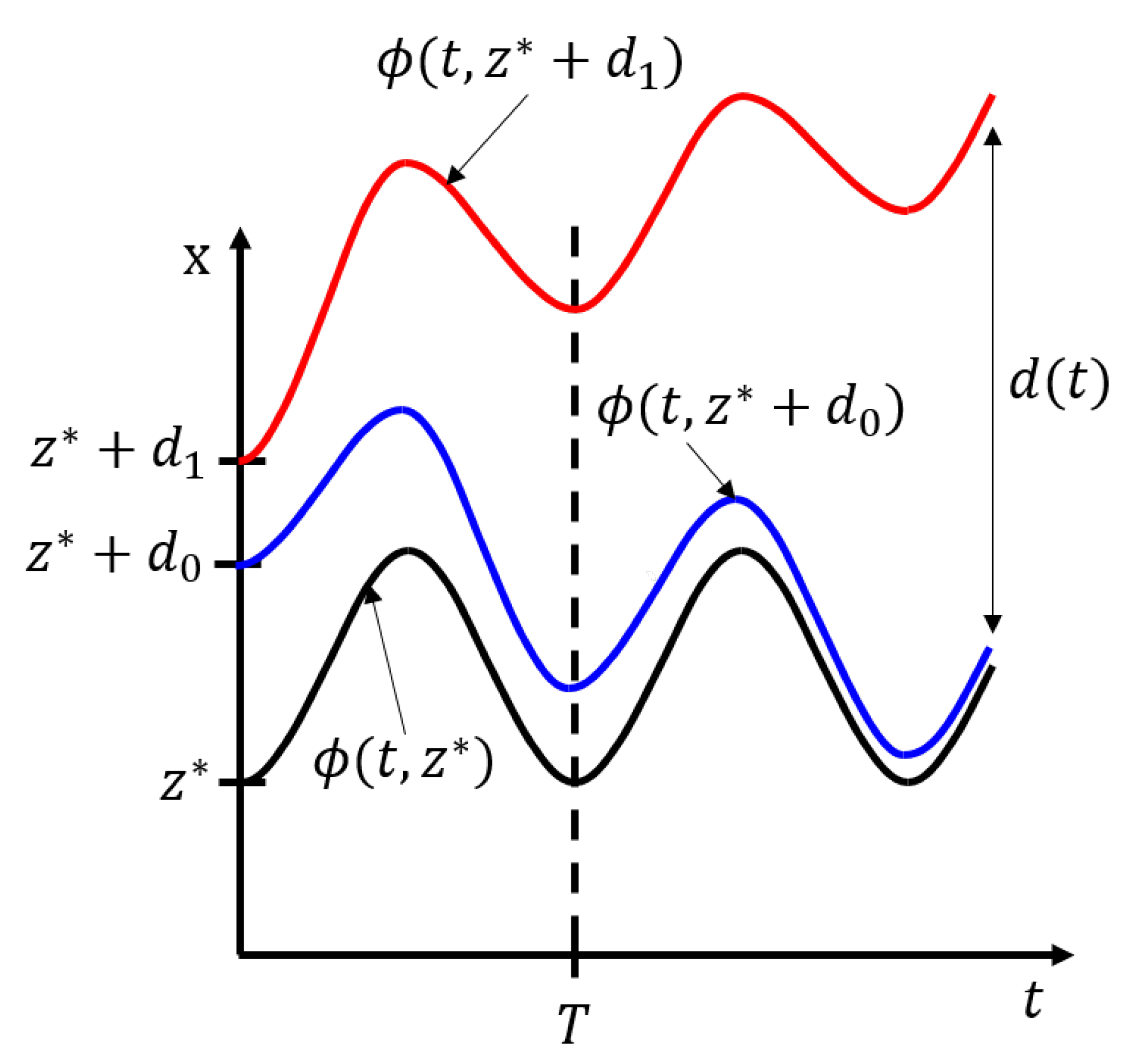The distance between trajectory progression and the periodic orbit is

$$\begin{array}{c}\hfill d(t)=\varphi (t,z^{\ast }+d_0)-\varphi (t,z^{\ast })\end{array}$$

(2)

where $z^{\ast }$ is the specific initial value for a specific solution. The distance with each period T is calculated by $d(T)$ and the linear representation with Taylor expansion becomes

$$\begin{array}{c}\hfill d(T)=\frac{\partial \varphi (T,z^{\ast })}{\partial z}{d}_0\end{array}$$

(3)

This linear approximation is not applicable to large disturbances such as $d_1$ in Figure 1. In Equation (3), the matrix

$$\begin{array}{c}\hfill M=\frac{\partial \varphi (T,z^{\ast })}{\partial z}\end{array}$$

(4)

governs the growth or decay as the initial disturbance $d_0$ is applied to the periodic solution. The matrix form of Equation (4) is the monodromy matrix. The characteristics of monodromy matrix are directly related to the behavior of the periodic solution and determined by its eigenvalues [7].

2.2. Poincar é Map

The Poincaré map construction is powerful geometric approach for studying the dynamics of various periodic phenomena. Specifically, some approaches start with phase portrait and its Poincaré section can be related to periodic stability results. The Poincaré map can be applied to n-dimensional differential equations. The set $\mathsf{\Omega }$ must be an $(n-1)$-dimensional hypersurface, satisfying a specific condition based on n-dimensional vector space. All orbits crossing $\mathsf{\Omega }$ in a $q^{\ast }\in \mathsf{\Omega }$ should meet two requirements:

(a)

The $\mathsf{\Omega }$ is intersected by orbits transversally

(b)

Orbits cross $\mathsf{\Omega }$ in the same direction

The $\mathsf{\Omega }$ can be characterized by the requirements as a local set of the trajectory. For instance, another $\mathsf{\Omega }$ for each period T can be driven by choosing another q point. The hypersurface $\mathsf{\Omega }$ is the Poincaré section. The subsets of planes are important class of $\mathsf{\Omega }$. The $\mathsf{\Omega }$ in $z\in {\mathbb{R}}_n$ is intersected by periodic trajectory y with period T. The $z^{\ast }$ can be represented as $q^{\ast }$ in a coordinate system on $\mathsf{\Omega }$, where q is $(n-1)$-dimensional. As $\varphi$ is restricted to $\mathsf{\Omega }$, this can be summarized as

$$\begin{array}{c}\hfill q^{\ast }=\varphi (T;q^{\ast })\end{array}$$

(5)

The time taken for an orbit $\varphi (t;q)$ to first return to $\mathsf{\Omega }$ is defined as $T_{\mathsf{\Omega }}(q)$ with $q\in \mathsf{\Omega }$.

$$\begin{array}{c}\hfill \varphi (T_{\mathsf{\Omega }}(q);q)\in \mathsf{\Omega },\varphi (t;q)\notin \mathsf{\Omega },\mathrm{for}0<t<T_{\mathsf{\Omega }}(q)\end{array}$$

(6)

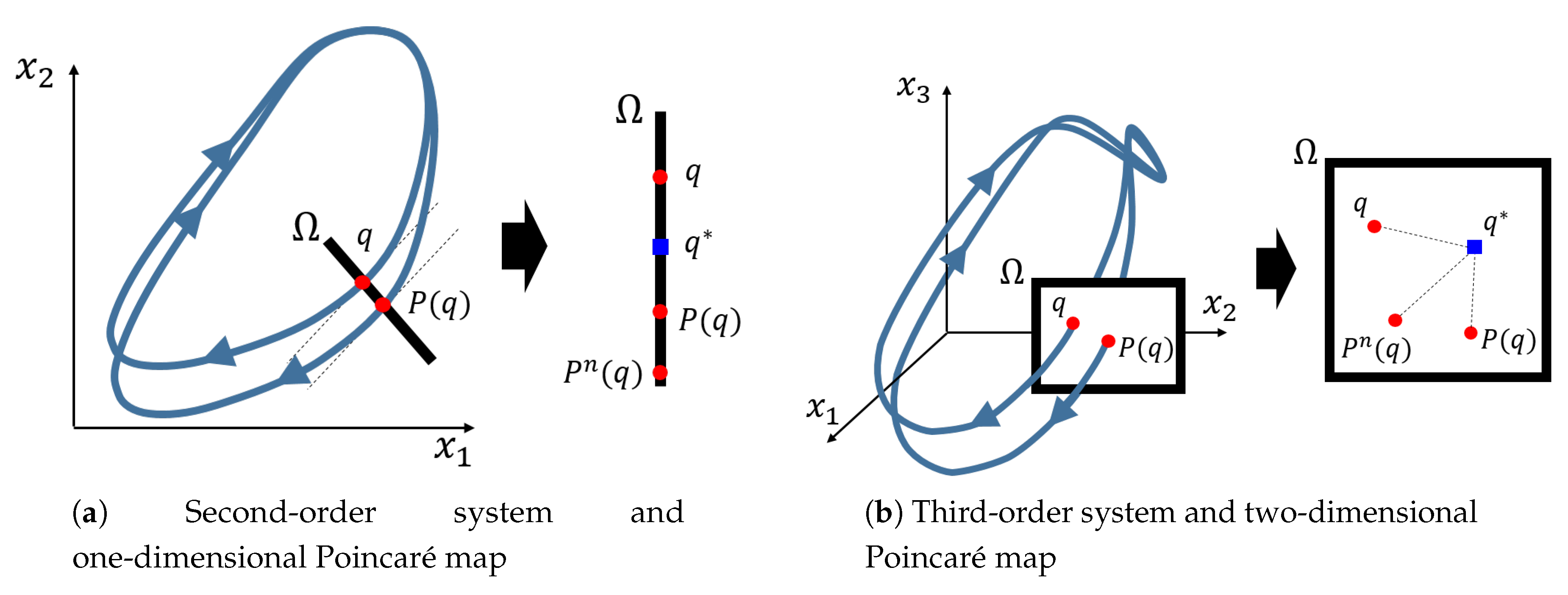
Poincaré map or return map $P(q)$ can be defined by

$$\begin{array}{c}\hfill P(q):=P_{\mathsf{\Omega }}(q)=\varphi (T_{\mathsf{\Omega }}(q);q),\mathrm{for}q\in \mathsf{\Omega }\end{array}$$

(7)

Figure 2a,b illustrate the geometric representation of $P(q)$.

2.3. Stability on the Periodic Orbits

In this section, the stability of one particular solution $x^{\ast }$ or $\varphi (t,z^{\ast })$ with period T along the periodic branch is investigated. The monodromy matrix $M(\lambda )$ has n eigenvalues ${\mu }_1(\lambda ),{\mu }_2(\lambda ),\cdots ,{\mu }_n(\lambda )$ with a value of $\lambda$ in (1), t; these eigenvalues are called Floquet multipliers. The magnitude in one of them can be always equal to unity. The other $(n-1)$ Floquet multipliers can determine local stability by applying following rule [7]:

• $x(t)$ is stable if $|{\mu }_j|<1$ for $j=1,\cdots ,n-1$.
• $x(t)$ is unstable if $|{\mu }_j|>1$ for some j.

The $(n-1)$ multipliers should be always inside the unit circle on the stable periodic trajectory. The multipliers are functions of the variables under deliberation. Crossing points between some of multipliers and the unit circle may exist as the parameter is varied. The critical multiplier can be defined as the multiplier crossing the unit circle. The multiplier crossing the unit circle is called the critical multiplier.

For a geometric interpretation, these Floquet multipliers can be expressed for the Poincaré section $\mathsf{\Omega }$. As defined by Equation (6), $P(q)$ not only q takes values in $\mathsf{\Omega }$, which is $(n-1)$-dimensional. The interpretation of both q and $P(q)$ is to have $(n-1)$ elements with respect to an appropriately chosen basis. The Poincaré map should satisfy

$$\begin{array}{c}\hfill P(q^{\ast })=q^{\ast }\end{array}$$

(8)

where $q^{\ast }$ is a secured point of P. The q is closer to $q^{\ast }$ as $T_{\mathsf{\Omega }}(q)$ is closer to the period T. The behavior of the Poincaré map can be near its secured point $q^{\ast }$ as a reduction of stability in the periodic trajectory $x^{\ast }$ occurs. Hence, the fixed point $q^{\ast }$ provides data on stability and can be an indicator to distinguish whether it is attracting or repelling. Similar to Equation (2), the unknown $P(q)$ can be described in Taylor series expansion.

$$\begin{array}{c}\hfill P(q)=P(q^{\ast })+\frac{\partial P(q^{\ast })}{\partial q}(q-q^{\ast })+\mathrm{higher}-\mathrm{order}\mathrm{terms}\end{array}$$

(9)

As q and $P(q)$ are in the hypersurface $\mathsf{\Omega }$, the number of elements in the linear approximated matrix $\partial P(q^{\ast })/\partial q$ is $(n-1)\times (n-1)$. The ${\mu }_1,\cdots ,{\mu }_{n-1}$ is defined as the eigenvalues in linearization of P as it is near the fixed point $q^{\ast }$,

$$\begin{array}{c}\hfill \mathrm{eigenvalue}\mathrm{of}({\mu }_j)\frac{\partial P(q^{\ast })}{\partial q},j=1,\cdots ,n-1\end{array}$$

(10)

Monodromy matrix and Poincaré surface are defined for the periodic solution. Thus, the selection of $\mathsf{\Omega }$ is not dependent on eigenvalues of the matrix. i.e., the eigenvalues will be the same regardless of the choice of point q. Hence, corresponding one set of eigenvalues ${\mu }_j$ exists for each periodic trajectory. Then, the eigenvalues determined from $\mathsf{\Omega }$ are also Floquet multipliers or (characteristic) multipliers, and a property of stability can be treated equally.

The $n^2$-monodromy matrix (8) has $+1$ as an eigenvalue with eigenvector ${\dot{x}}^{\ast }(0)$ tangent to the intersecting curve $x^{\ast }(t)$. The eigenvector ${\dot{x}}^{\ast }(0)$ is not in hypersurface $\mathsf{\Omega }$ since the property of that intersection point should cross transversally. The eigenvalue $+1$ in the monodromy matrix matches up with an agitation along $y^{\ast }(t)$ leading out of $\mathsf{\Omega }$. while the other $n-1$ eigenvalues in the monodromy matrix can decide what occurs to small agitation within $\mathsf{\Omega }$. In summary, choosing the proper basis for the n-dimensional space shows that the remainder of $n-1$ eigenvalues of M match the eigenvalues of $\partial P(q^{\ast })/\partial q$.

3. Estimated Floquet Multipliers in Time Series Data

In the previous section, a system is dealt with a specified mathematical model. Here, we address the case of measurement-based or time series data when the equation or model is unknown. First, deciding on the proper form of the Poincaré map for time series data that corresponds to the original Poincaré map is required. Then, we can estimate the Floquet multiplier by the linearized form of the equation.

3.1. Poincar é Map Construction for Time Series Data

As discussed in Section 2, Reference [7] gives some guidelines for constructing a Poincaré map for time series data. These focus on the data quality of the constructed Poincaré map. It is a fact that the Poincaré surface should include information on the cycle. A specific procedure to construct a data-based Poincaré surface is presented in the following subsection.

3.1.1. Poincar é Surface Decision for Time Series Data

Two requirements in choosing hyperplane $\mathsf{\Omega }$ have been provided in the previous section. At $\mathsf{\Omega }$, transversally intersecting points should have the same direction. For continuous values, these conditions are conceptually reasonable. However, it is hard to choose a Poincaré surface when discrete values are given. The direction corresponds to differential values of the trajectory and the transversality condition matches the local intersection. Thus, the Poincaré map in time series data should fulfill these two conditions, where $\varphi$ is a periodic trajectory in discrete values, x is all the points in the trajectory $\varphi$, and $\alpha$ is a differential value that has to be determined.

(a)

Transversality $x_{\mathsf{\Omega }1}=\{x|x_a\le x\le x_b,x\in \varphi \}$

(b)

irection $x_{\mathsf{\Omega }2}=\{x|\dot{\varphi }\approx \alpha ,x\in \varphi \}$

Therefore, the points included in the Poincaré surface are the intersection of two sets $x_{\mathsf{\Omega }1}$ and $x_{\mathsf{\Omega }2}$. The problem of constructing the Poincaré surface for time series data has been converted into a problem of choosing $x_a$, $x_b$, and $\alpha$. First, using engineering-based judgment, it is safer for discrete data to set $\alpha$ as zero. Reference [8] supports the notion that the (numerical) time derivative of the signal is a legal coordinate in a reconstructed state space for scalar data that contains some information on the original state space. Hence, the time derivative for scalar s might provide information on the direction. $\dot{s}=0$ is precisely given by the local minima (or maxima) of the time series. In addition, the local minima (or maxima) are interpreted as the special measurement function which projects onto the first component of a vector applied to the state vectors inside surface $\mathsf{\Omega }$. It is experimentally acceptable that the local peak values when $\dot{\varphi }\approx 0$ have less errors than other slopes of the trajectory.

Once the trajectory crosses $\mathsf{\Omega }$, the next intersecting point in the same direction is acquired after the 1 cycle. In Figure 2a, the period leading point $P(q)$ is on the same line as the period lagging point q. Similarly, third-order systems can be generalized to the two-dimensional hyperplane $\mathsf{\Omega }$. Since there is neither a mathematical model nor cycle T given for the time series data, specific points that can be regarded as intersection points of $\mathsf{\Omega }$ need to be selected. For the second-order system in Figure 2a, the line might be clearly chosen at two peak points in ${\dot{x}}_2=0$ from a point of the requirements for choosing the Poincaré surface. Similar behaviors in Figure 2b, however, show that there are four peak points ${\dot{x}}_3=0$ to be selected. In this case, the lower local minima are the best candidates to choose the Poincaré surface.

For measured data for an arbitrary system, the values of $x_a$ and $x_b$ for condition (a) transversality are naturally decided, such that $x_a$ are values near zero and $x_b$ is the median value of measured data from the conceptual sketch in Figure 3. Then, two conditions for Poincaré map decision-making can be expressed as

All local minima sets less than the median value are included in the Poincaré map $\mathsf{\Omega }$.

Figure 3 explains the concept of Poincaré map construction for time series data in an arbitrary system. When the measured data for $x_1$ are given, the peak points marked in red stars and blue rectangular points are found by applying the peak searching algorithm. Then, the sorted peak points under the computed median of $x_1$ are ready to estimate the Floquet multiplier.

For example, for the three-bus system given in [14,15], when setting the load bus reactive power of 10.946 MVar as a parameter, a pure four-dimensional periodic return map is acquired. Then, for 100 samples of local minima set $p_l$, the standard deviation of the state variables $\delta$, $\omega$, ${\delta }_L$, and V are $5.43\times {10}^{-6}$, $9.80\times {10}^{-5}$, $1.79\times {10}^{-6}$, and $7.16\times {10}^{-8}$, respectively. These small standard deviations show that the 100 sample points of local minima are a fixed point. As the fixed point is defined in the Poincaré surface $\mathsf{\Omega }$, the local minima set is in the Poincaré surface $\mathsf{\Omega }$.

3.1.2. Effect of Dimension Reduction by Projection

For a higher-order system which is hard to visualize, such as a fourth-order system, it is still possible to imagine the three-dimensional Poincaré section. Assume that all local minima are the values when one of the state variables satisfies $x_4=c$, where c is a constant value. Then, the three-dimensional axis of the Poincaré section will be $x_1,x_2$, and $x_3$. If the measured oscillatory behavior is purely periodic, not only $x_4$ but also the three variables $x_1,x_2$, and $x_3$ would be fixed. However, when the three variables change for every cycle, checking the three variables at once and monitoring the measured value of local minima will not be the same.

Using the local minima searching concept stressed above, a set of local minima or intersection points are identified inside a three-dimensional box. At the first projection in Figure 4, the average distance between each point decreases. Then, another projection makes the points stick to the axis of the measured value. Hence, there apparently exists an inevitable gap between the three-dimensional Poincaré map and the double projected local minima of the time series data. As mentioned in Section 3.1.1, the standard deviation is small when the trajectory is stable, and projection will have no effect. The gap will only affect the results when the trajectory is unstable, especially for higher-order systems.

3.2. Floquet Multiplier Estimation

In Section 2.3, the matrix $\partial P(q^{\ast })/\partial q$ is provided by the monodromy matrix with restriction to the $n-1$-dimensional hyperspace $\mathsf{\Omega }$. The $P(q)$ can be expressed by Taylor series in the vicinity of the fixed point $q^{\ast }$. Assuming that periodic solution is stable, higher-order term can be negligible. Recalling that $P(q^{\ast })=q^{\ast }$ at the fixed point, Equation (10) is linearized as

$$\begin{array}{c}\hfill P(q)-q^{\ast }=[\frac{\partial P(q^{\ast })}{\partial q}](q-q^{\ast })\end{array}$$

(11)

For the specific vector $q_1$, the corresponding critical eigenvalue ${\mu }_1$ is calculated using the linear approximated equation

$$\begin{array}{c}\hfill P(q_1)-q^{\ast }={\mu }_1(q_1-q^{\ast })\end{array}$$

(12)

If we have series data x, the relationship between the mapping P of point q and point q can be followed by sequence $x[k]$ and $x[k+1]$. Hence, the computational form gives Equation (11) by

$$\begin{array}{c}\hfill x[k+1]-x^{\ast }=\widehat{\mu }(x[k]-x^{\ast })\end{array}$$

(13)

Equation (12) is a typical form of linear regression, where $\widehat{\mu }$ is a constant to be determined by series data x.

For application to time series data, the equation should be modified to a scalar form. In that case, the calculated Floquet multiplier might not be the same as the actual value since the scalar value cannot reflect the direction. However, there will be negligible differences when selecting the acceptable component of the state variable. Using engineering judgment, it will be natural to select the component with the largest variance among the state variables x.

$$\begin{array}{c}\hfill s[k+1]-s^{\ast }={\widehat{\mu }}_F(s[k]-s^{\ast })\end{array}$$

(14)

The estimated Floquet multiplier ${\widehat{\mu }}_F$ can be easily computed with Equation (10). The estimated value, however, is not the exact value of the calculated Floquet multiplier because it is estimated and projected in one dimension, regardless of the number of original system state variables it contains. But as long as the signal is periodic, the estimated Floquet multiplier gives information on stability even if we choose single measurement as a state variable.

For application to time series data, Equation (13) can be expressed after changing scalar s to voltage term V

$$\begin{array}{c}\hfill {\widehat{\mu }}_{F,series}=\frac{1}{N}\sum _{k=1}^N\frac{V[k+1]-(1-\mu )V^{\ast }}{V[k]}\end{array}$$

(15)

Ironically, the linearized form of Equation (13) contradicts the stable orbits when $s[k+1]\approx s[k]\approx s^{\ast }$. Hence, the $\mu$ term of Equation (14) should be 1 by applying the stable orbit condition.

$$\begin{array}{c}\hfill {\widehat{\mu }}_{F,series}=\frac{1}{N}\sum _{k=1}^N\frac{V[k+1]}{V[k]}\end{array}$$

(16)

Then, the final estimation Equation (15) further simplifies the problem such that the estimated Floquet multiplier is only the average of the ratio of the previous and current local minima of the voltage at all peak data. In other words, we can set the fixed-point value to zero. It can be guaranteed that ${\widehat{\mu }}_{F,series}=1$ is a sufficient condition for stable orbit. Using final Equation (15), other unstable cases are demonstrated by two examples of power systems in Section 4.

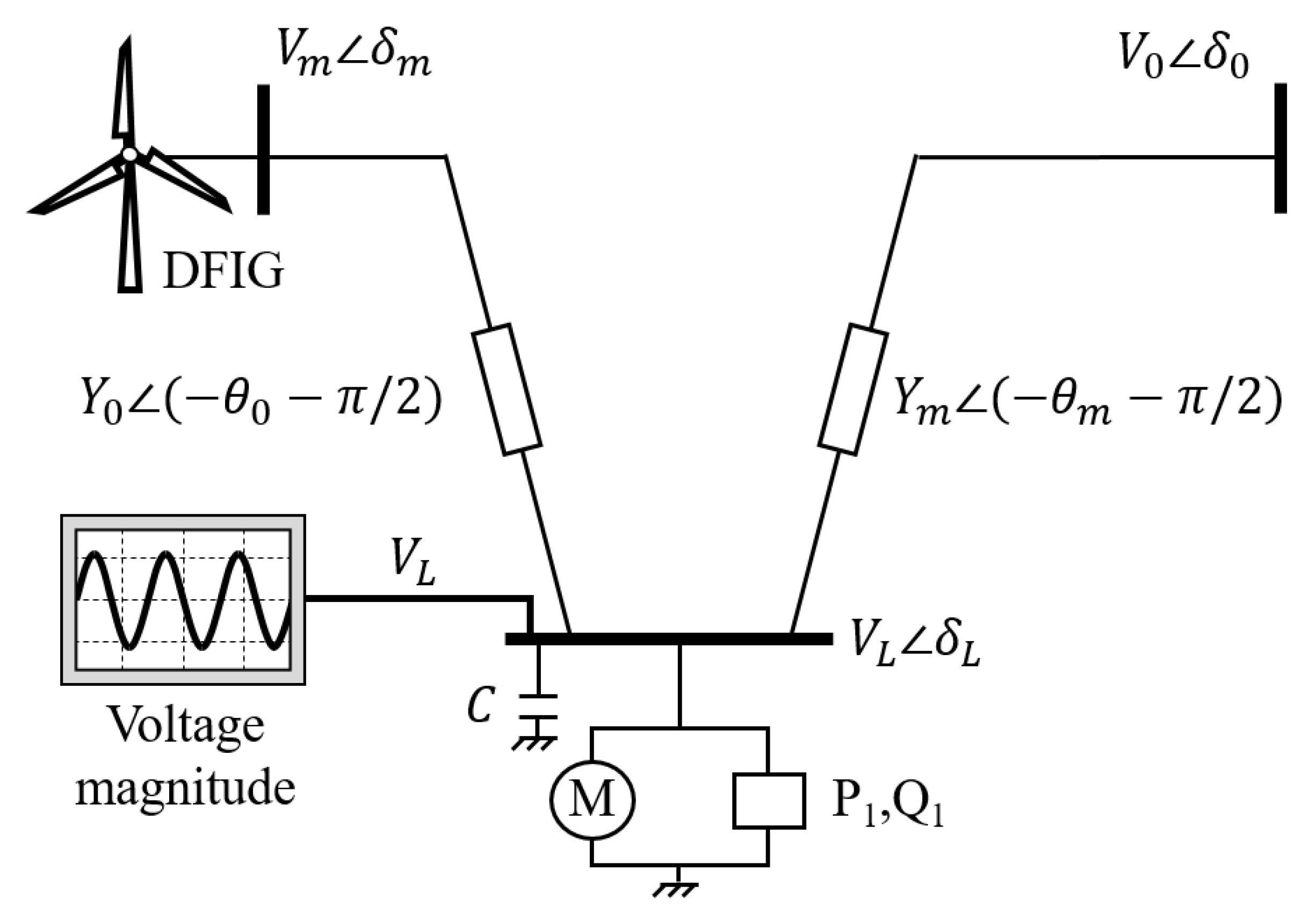
4. Power System with DFIG

In this section, comparative studies of the calculated and estimated Floquet multipliers for two cases are performed. Starting with the mathematical modeling of a power system with DFIG, the application of the suggested method in test power systems and power system with a complicated DFIG model are studied.

The modeling of a DFIG is not as simple as a general synchronous generator. The state matrix of the system becomes larger, considering not only the characteristics of controllers but also the complexity of the machine. The specified model of the DFIG is provided with network equations in the appendix of [16]. In this paper, Floquet multiplier have been estimated under even more complex system. That is, DFIG model of [16] is added to the three-bus system with induction motor which have been constructed at [15]. The specified model of this system is provided at Appendix A.

Figure 5 shows a three-bus power system network with the DFIG installed at bus 3. Time series voltage data in rms were obtained at the load bus. The Floquet multiplier was estimated for the results of the time domain simulation of $V_L$. The bifurcation diagram of power grid with DFIG is represented in Figure 6, which was determined by the mathematical model of the system. The mathematical model for the system containing aerodynamics and electric power system dynamics are given as follows:

In Figure 6, from the left Hopf bifurcation point 8.669 MVar to right Hopf bifurcation point 11.33 MVar, periodic solutions exist where the amplitudes of the orbit are large in the middle of the range. Before estimating the Floquet multiplier in the power system with DFIG, the sample three-bus power grid was examined.

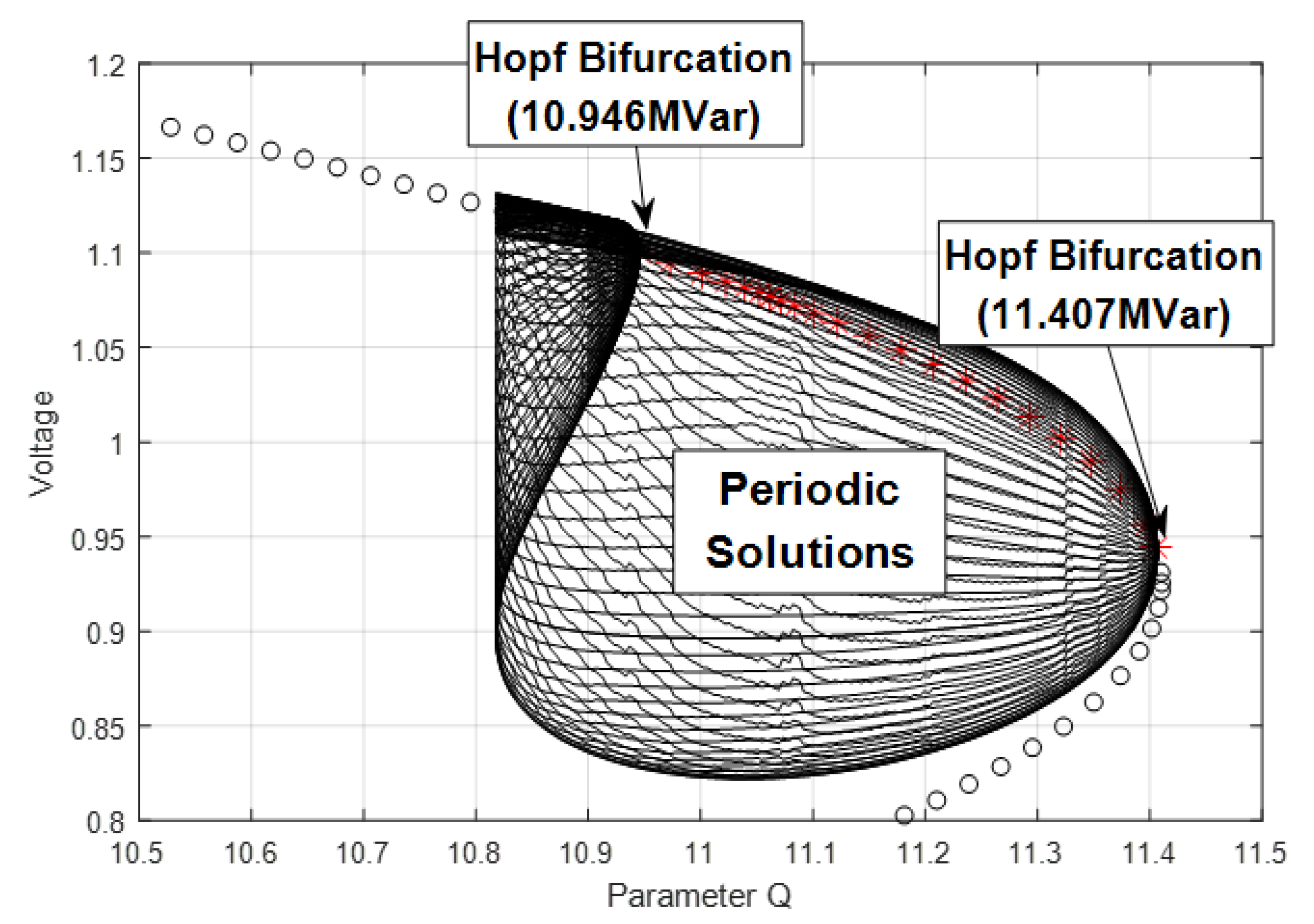
Similar to the previous case, the three-bus power grid in [14,15,16] showed two Hopf bifurcation points. Periodic orbit can be observed in parameter $Q_1$ from 10.946 MVar to 11.407 MVar in Figure 7. Time domain simulations were performed in between these two bifurcation points to check nonlinear oscillatory behaviors. The Floquet multiplier was calculated by the monodromy matrix of the system and the corresponding Floquet multiplier was estimated for comparison with the critical multiplier.

4.1. Calculated Floquet Multiplier in Sample Power System

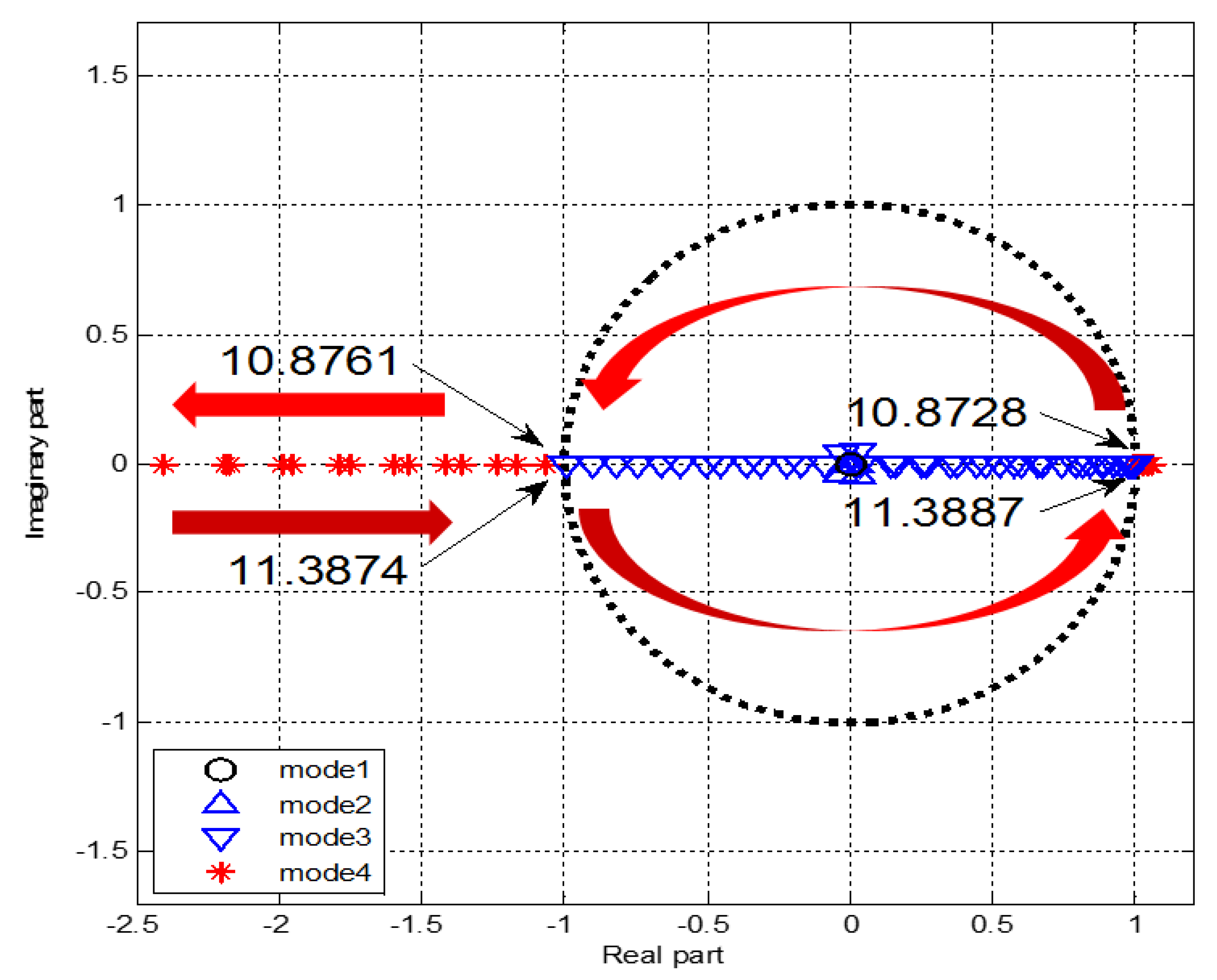
In Figure 8, four modes of the Floquet multiplier are calculated and the trajectories of these modes are described. Mode 1 is always zero, while the other modes move inside the unit circle. When the parameter increases at 10.946 MVar, the critical multiplier in mode 4 stays on the right side of the unit circle until 10.8728 MVar; then it moves to the left side of the circle with a slight change in parameter. This is the point where the periodic solution of the system loses stability. Without stopping, the critical multiplier moves to the left along the real axis approximately −30, and then changes direction and heads to the unit circle. The value when the trajectory meets the unit circle is 11.3874 MVar and moves to the right side of the circle with a small change at 11.3887 MVar.

4.2. Estimated Floquet Multiplier in Sample Power System

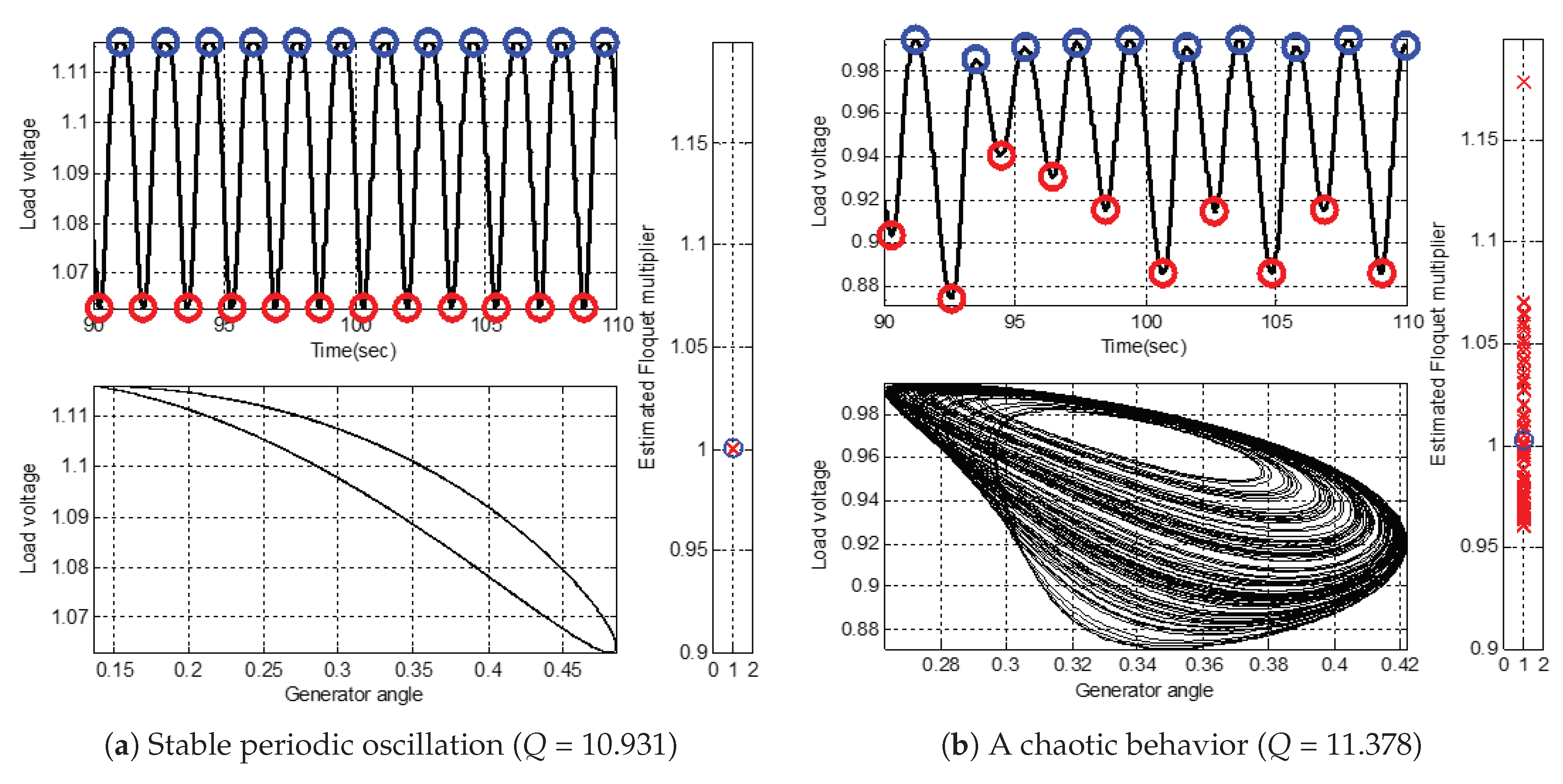
Figure 9a,b shows the rms voltage values at the load bus (left-top), phase portraits of the generator angle and load voltage (left-bottom), and Floquet multiplier estimation (right) for specific parameter values. Stable oscillatory behavior is observed in Figure 9a. The local minima of the rms voltage marked in red circles appear to be steady. The phase portraits on the left-bottom show that the trajectory of the solution is in the attractor. On the right side of the picture, the points marked in red crosses are the values related to $V[k+1]/V[k]$ in Equation (15). The estimated value was determined from the average of these values.

The left-bottom of Figure 9b shows that the periodic solution is still inside the attractor, but the orbit is inconsistent. Figure 9b is obviously an unstable periodic solution such that ratio $V[k+1]/V[k]$, which are marked in red crosses, are scattered from 0.96 to 1.18. The average of these points is 1.002, marked in blue circles. To summarize the sample cases for Figure 9a ($Q_1$ = 10.931 MVar), the estimated and calculated values are 1 and 1.005, respectively. For Figure 9b ($Q_1$ = 11.378 MVar), the estimated and calculated values are 1.0023 and −2.317, respectively.

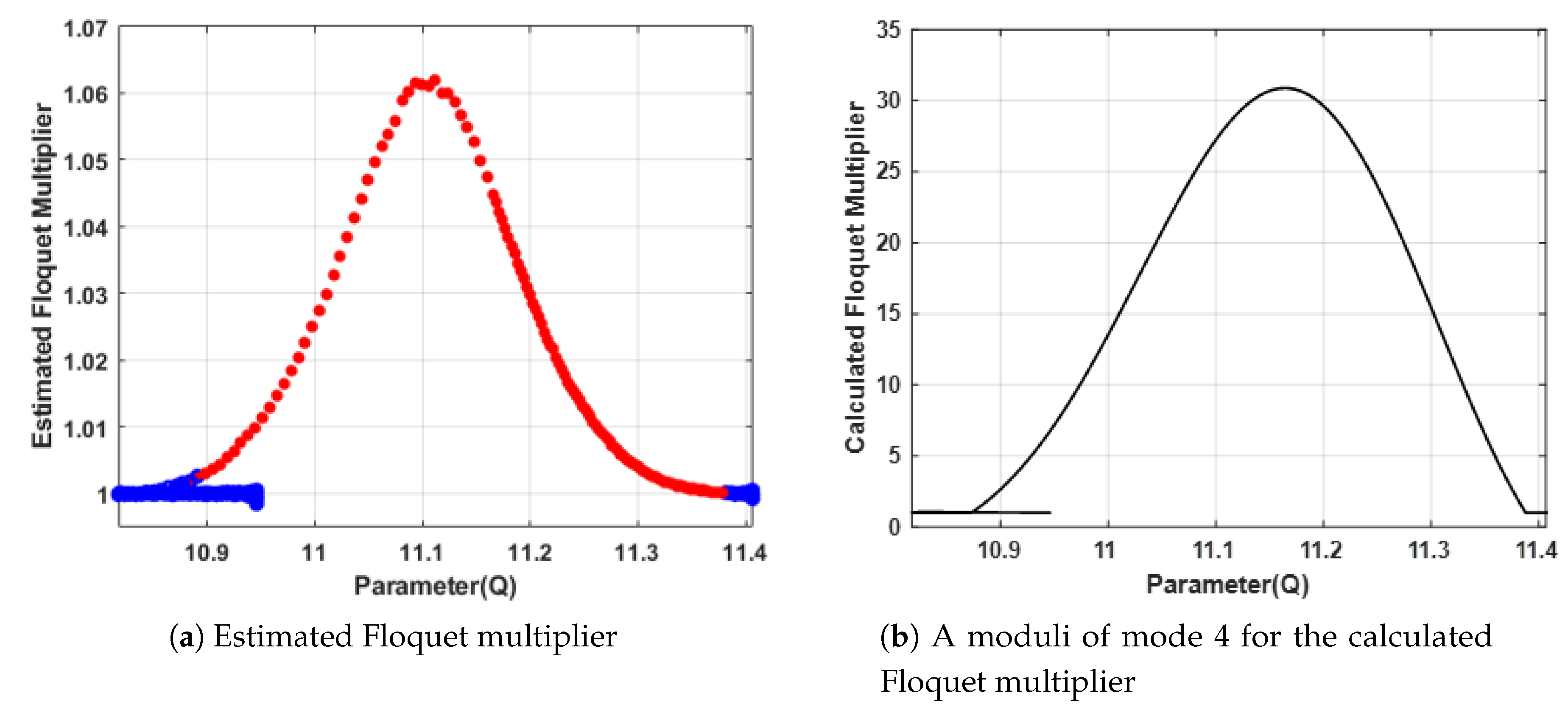
To apply Equation (15), at least two local minima are required. We set a three-cycle time interval for the ordinary differential equation (ODE) tool from MATLAB (R2014a, Mathworks, Netic, MA, USA). For the three-cycle time series data of all parameter ranges, the Floquet multipliers were estimated using Equation (15). In Figure 10a, the overall values are not as large as the moduli of the calculated Floquet multipliers. The points marked with blue dots are the points which are near unity, while the points marked with red dots are the points when the deterministic Floquet multiplier goes outside the unit circle. The estimated Floquet multiplier has unity value when the deterministic Floquet multiplier calculated from monodromy matrix is stable (unity), as shown in Figure 10a. Likewise, the estimated Floquet multiplier is greater than unity when the moduli of the deterministic Floquet multiplier are unstable (greater than one), as shown in Figure 10b. The correlation coefficient between two results Figure 10a,b for partial interval are 0.824.

Comparing the two approaches shows that the estimated Floquet multiplier using Equation (15) gave similar information on a short-term signal. The boundary of stability was less likely to be observed in the estimated Floquet multiplier, while the actual calculated Floquet multiplier changed its sign upon losing stability.

4.3. Comparison between Estimated Floquet Multiplier and Calculated Floquet Multiplier

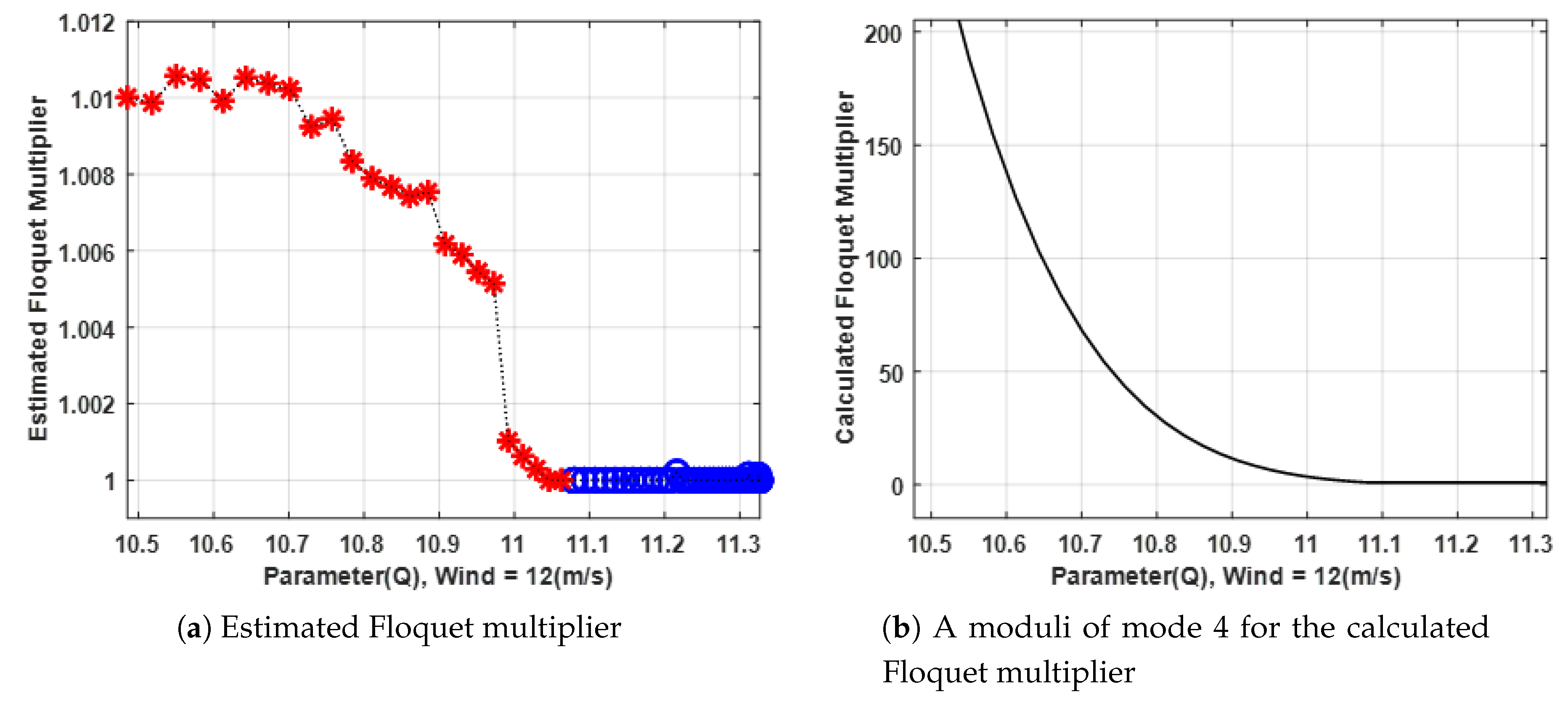
Figure 11a shows an estimated (data-driven) Floquet multiplier and Figure 11b shows the calculated (model-based) Floquet multiplier of test power system with DFIG. For a higher-order system, the estimated Floquet multiplier values remained near unity when these were calculated with the monotomy matrix inside the unit circle. When the calculated Floquet multipliers were about to lose their stability, the estimated Floquet multiplier values stayed at approximately 1 from 10.993 to 11.064 MVar. Then, the estimated Floquet multipliers increased in the positive direction although this was not as large as the calculated values. Likewise, the calculated Floquet multipliers dramatically decreased in the negative direction. Once the estimated Floquet multiplier lost stability, it also lost its increment tendency, i.e., stiff growth was observed from 10.604 to 10.635 MVar, 10.781 to 10.807 MVar, and 10.973 to 10.993 MVar. The correlation coefficient between two results Figure 11a,b for partial interval are 0.758. Specifically, the proposed method accurately estimated the Floquet multiplier as long as the oscillation behavior was purely periodical.

5. Actual Oscillation Incident

In this section, estimated Floquet multiplier is calculated to actual oscillation event observed in New England ISO in 17 June 2016. The oscillation was system wide and the frequency of 0.27 Hz, 27 MW peak-to-peak. The location of the source was far away outside of interested area. PMU data was acquired for 3 min, and actual event kept going for 140 s. For data preprocessing, original current data was subtracted to its averaged value. Average values are calculated by 162 samples of moving window considering a period is approximately 8 samples and its quarter at sampling rate of 0.033 s. So the signal oscillates around zero for the current PMU data of 35 locations. And the oscillation is clearly observable at 24 locations. Figure 12a shows example actual current minus average current value with noise at transmission line near substation 6. The local maxima have been well detected but still the peak values are fluctuations of Floquet multiplier of 1.045. Figure 12b shows a simple map of New England ISO with all estimated Floquet multiplier marked on it. It is clear that area marked in yellow has high value than other line currents. Even the line connected substation 9 and external area has the highest value of all. So the oscillation source for this incident can be traced through external area. Overall estimated Floquet multiplier is 1.0396, which can be judged that the system wide oscillation is unstable periodic solution mathematically. However, considering the real power system, Floquet multiplier of the oscillation can be shown slightly higher than 1.0 due to load fluctuation or generator excitor operation.

6. Discussion

According to the results of both cases in the previous section, the estimated values followed a similar trend as the calculated values. However, in general, the estimated values were not as large as the calculated values. For the power system with wind generator, the estimated Floquet multiplier lost a pattern of increment once it lost stability. There are several possible reasons that can explain this outcome.

(1) Dimension reduction by projection

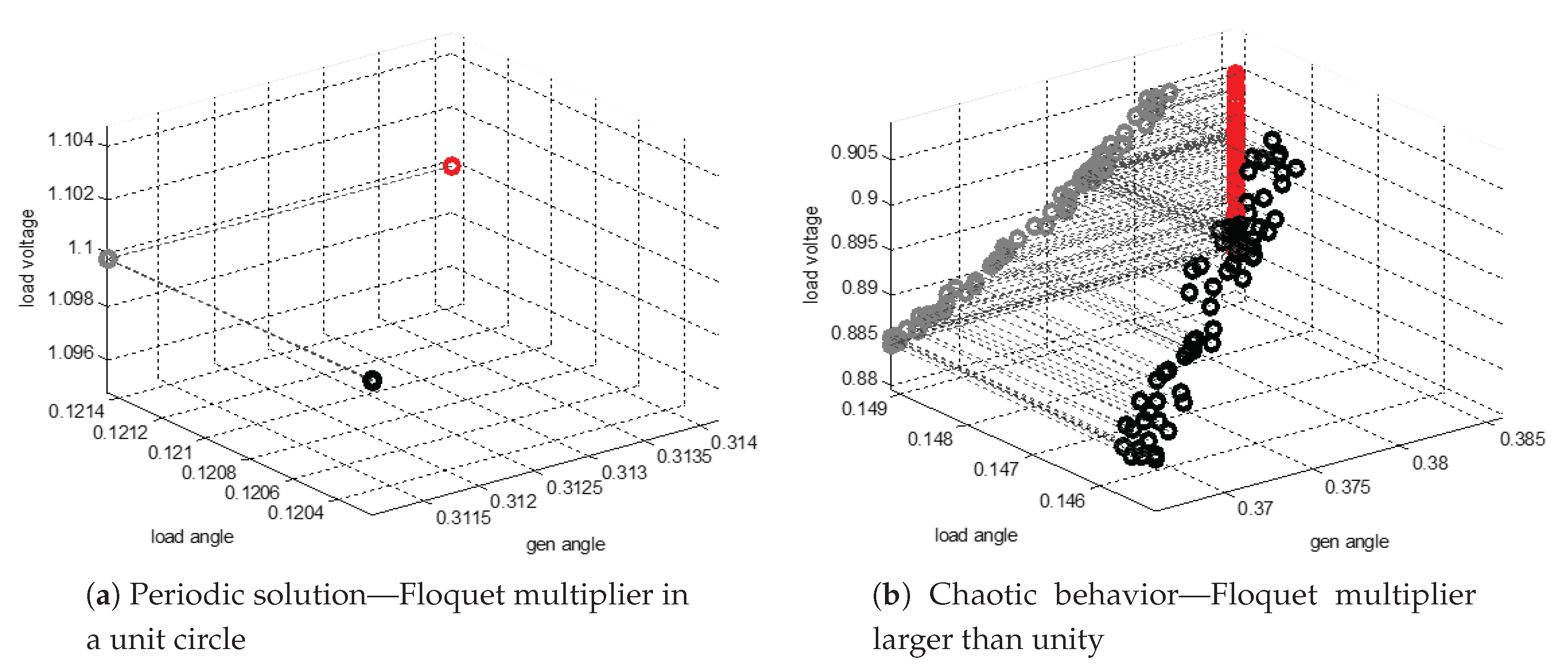
The proposed method is targeted to use local phasor measurement unit data from power systems. Thus, estimating the Floquet multiplier is strictly limited to time series data in one-dimensional space. Figure 13a,b shows the three-dimensional intersection in the Poincaré section and their projections onto one-dimensional line and chaotic behavior, respectively. Figure 13a is a typical limit cycle oscillation. Clearly, no distortions occurred. Moreover, when the measured data showed period doubling, the projection of two intersections onto the three-dimensional hyperplane $\mathsf{\Omega }$ may start to reveal unintended differences.

Figure 13b shows the results of chaotic behavior. For the sample three-bus power system, distortion occurred for a step of projection. Initially, the three-dimensional intersections were scattered on the space. The projection onto a two-dimensional plane gave different values. Then, the projection onto a line, which was the result for time series data, yielded totally distorted values compared to the original intersection.

The power system with wind generator is a 10-dimensional system. The Poincaré surface would be nine-dimensional, thus projections will be carried out eight times. Then, ignoring the other axes, only the local minima of time series data would give the estimated value of the Floquet multiplier. Therefore, it is natural that the estimated Floquet multiplier is less than the calculated Floquet multiplier.

(2) Assumption of linearization

According to the proposed method introduced in Section 3.2, the estimating Equation (10) is linearized near $q^{\ast }$, which means that the equation assumes a stable periodic solution. However, if the solution loses stability or the Floquet multiplier goes out of the unit circle, then the assumption is void. i.e., the $(1-\mu )$ term of Equation (15) is no longer zero. Therefore, in a stable periodic region, the estimated Floquet multiplier shows the exact value of unity that we intended it to be, but there is a risk of error in the unstable periodic region. Although there are some error risks when the oscillation loses stability, we can easily recognize the unstable region where the estimated Floquet multiplier is greater than 1.

(3) Differential equation calculation limits

The numerical ODE solving tool is required to validate the calculated and estimated Floquet multipliers. For time domain simulation, the ODE45 tool of MATLAB was used. In some parameter ranges, the solution diverged within one or two cycles, which means that not enough local minima were gathered to construct the Poincaré surface. In real power system problems, the proposed method is aimed at sustaining oscillation measured by PMU. The computation of solution of Equation (1) is beyond the scope of the present study.

7. Conclusions

In this work, we compared a proposed method of estimating the Floquet multiplier with time series data and a calculated Floquet multiplier based on a mathematical model. We described how to construct a Poincaré map in time series data, starting with the definition of the Poincaré map. We stressed the possibility of disagreement between the calculated and estimated Floquet multipliers by projection concept. A linearized form of the Floquet multiplier was provided to estimate the time series data with period.

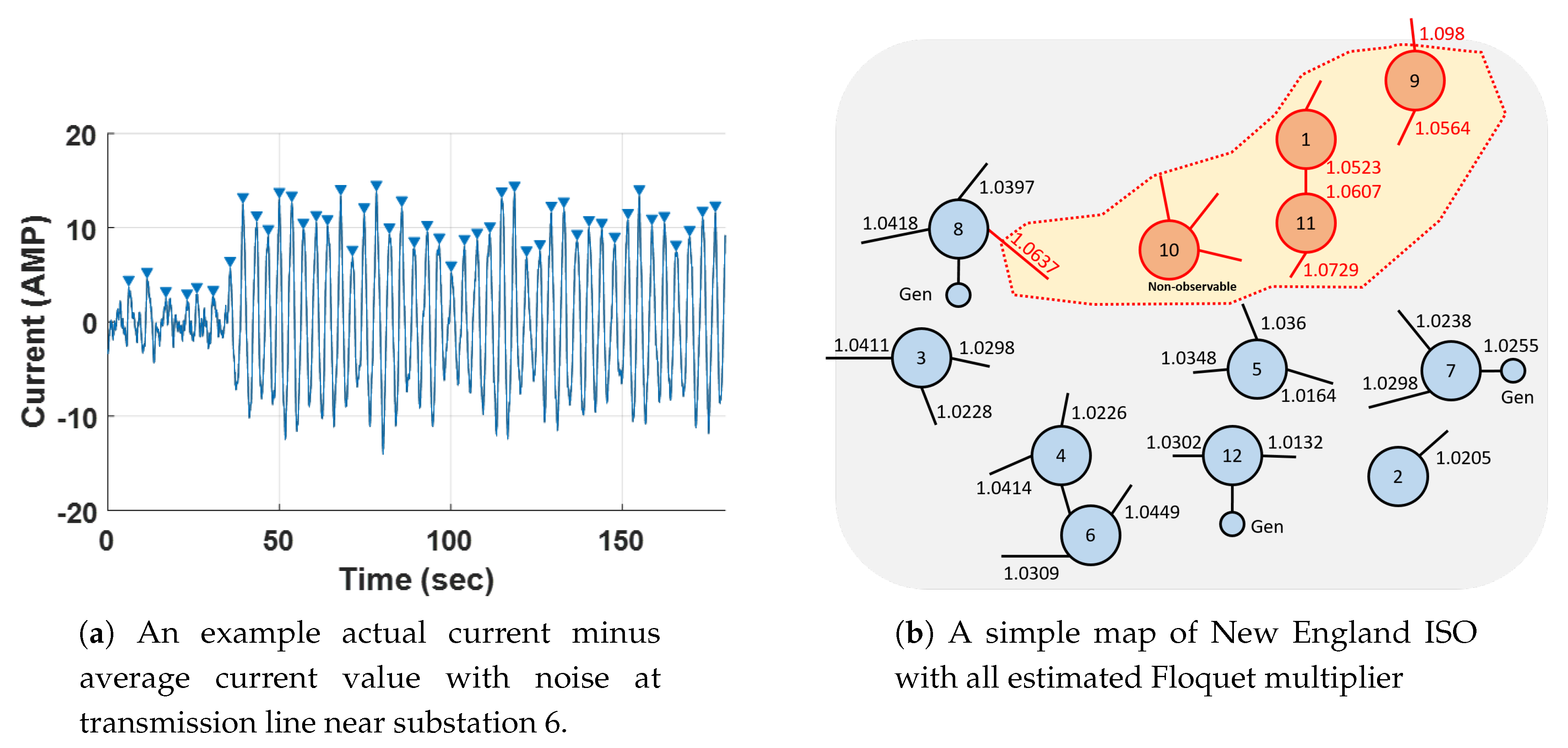
We found that the estimated Floquet multipliers followed a similar trend as the Floquet multipliers calculated with the monodromy matrix in two power system networks after conducting correlation analysis. A Poincaré map selected by a local peak value searching algorithm provided enough information on an arbitrary system by considering their standard deviation. Thus, the critical multiplier of the estimated value was unity for the stable oscillation. For practical application with noisy measurement, we have conducted Floquet multiplier estimation to actual oscillation incident. Results show that estimated Floquet multiplier is not exactly unity due to load fluctuation or generator excitor response. However, still the estimated Floquet multiplier act as an indicator for feature of sustained oscillation while the value could stand for signification of the oscillation sources. Therefore, the proposed method can successfully function as a period oscillation indicator for time series data acquired from power systems.