Article

Simulation and Analysis of Perturbation and Observation-Based Self-Adaptable Step Size Maximum Power Point Tracking Strategy with Low Power Loss for Photovoltaics

1
Department of Electrical and Electronic Engineering, Xi’an Jiaotong–Liverpool University, Suzhou 215123, China
2
Department of Architecture, Xi’an Jiaotong–Liverpool University, Suzhou 215123, China
*
Author to whom correspondence should be addressed.
Energies 2019, 12(1), 92; https://doi.org/10.3390/en12010092
Submission received: 15 November 2018 / Revised: 21 December 2018 / Accepted: 24 December 2018 / Published: 28 December 2018
(This article belongs to the Special Issue Energy Efficiency in Buildings: Both New and Rehabilitated)

Abstract

:
Photovoltaic (PV) techniques are widely used in daily life. In addition to the material characteristics and environmental conditions, maximum power point tracking (MPPT) techniques are an efficient means to maximize the output power and improve the utilization of solar power. However, the conventional fixed step size perturbation and observation (P&O) algorithm results in perturbations and power loss around the maximum power point in steady-state operation. To reduce the power loss in steady-state operation and improve the response speed of MPPT, this study proposes a self-adaptable step size P&O-based MPPT algorithm with infinitesimal perturbations. This algorithm combines four techniques to upgrade the response speed and reduce the power loss: (1) system operation state determination, (2) perturbation direction decision, (3) adaptable step size, and 4) natural oscillation control. The simulation results validate the proposed algorithm and illustrate its performances in operational procedures.

1. Introduction

1.1. Background

A direct current (DC) [1] pattern exists in almost all the electrical devices in our daily life. Photovoltaics (PV), as well-known renewable power generation solutions, are a foundational DC source which can supply DC power for DC application directly or drive the alternating current (AC) application after inverting. Owing to the policy support and sharp cost reduction of photovoltaic [2] techniques, solar power, a form of inexhaustible eco-friendly energy, has been widely exploited in daily life in recent years. At the same time, the civilization process enhances the demands of civil space. To increase the utilization of urban space, building-integrated photovoltaic techniques are becoming more widely considered in the research community [3,4,5,6,7,8,9,10].
Building integrated photovoltaics, a significant branch of PV generation, are easily affected by environmental conditions, similar to other PV applications. The output characteristics of the PV panel are mainly influenced by the illumination intensity, temperature, material, and other conditions, especially the received illumination intensity and the surface temperature of the PV panel. For example, increasing the temperature results in a slight increase in the short-circuit current and a significant decrease in the open-circuit voltage, which reduces the maximum output power. However, in any condition, a curve of the output power can be drawn, and the output power has a maximum output point called the maximum power point (MPP) [7,11,12,13,14,15,16,17,18,19,20,21,22]. For the PV system operated with higher efficiency, an MPP tracking (MPPT) controller is indispensable; the tracking methodologies are introduced in detail in the MPPT section of this report.
For a PV system with an MPPT controller, the structure can be depicted as consisting of a PV panel, a power converter [7,8,16,19,20,21,22,23,24,25,26,27,28,29,30,31,32,33], an MPPT controller, and a load (including but not limited to motors, batteries, heaters, energy-storage systems, and other electric appliances). The structure of the PV system is shown in Figure 1.
The operating process of the PV system can be simply explained as follows. After absorbing enough radiation, the PV panel supplies electricity to the power converter and the load is driven via the output from the power converter. Simultaneously, the MPPT controller measures specific parameters (such as voltage and current) for controlling the power converter in order to make the system operate at the MPP.

1.2. Aims and Objectives

This study discusses an advanced algorithm to improve the efficiency of the perturbation and observation (P&O)-based MPPT with simulation and numerical analysis tools. Power loss, a common phenomenon in electricity generation, refers to the power consumed during the conversion process; it is unavoidable, but can be reduced. For the conventional P&O-based MPPT controller of a PV system, certain power loss is caused by the ineluctable perturbation of the P&O method. If the power loss can be reduced, the utilization rate of the solar energy can be increased, and more energy can be saved.
To solve the power-loss problem caused by the non-environmental conditions causing oscillation, a P&O-based self-adaptable MPPT algorithm is designed in this study. This algorithm is expected to reduce the power loss and improve the response speed of tracking.

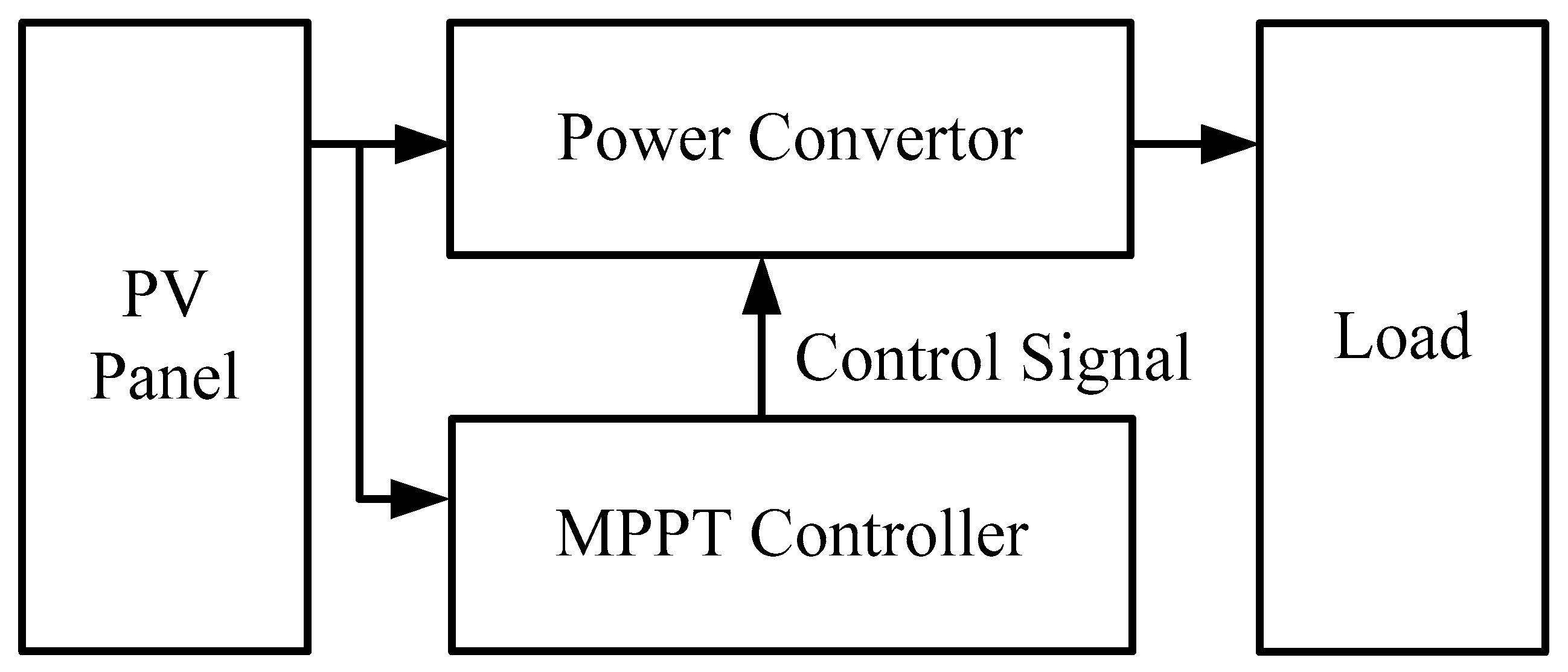
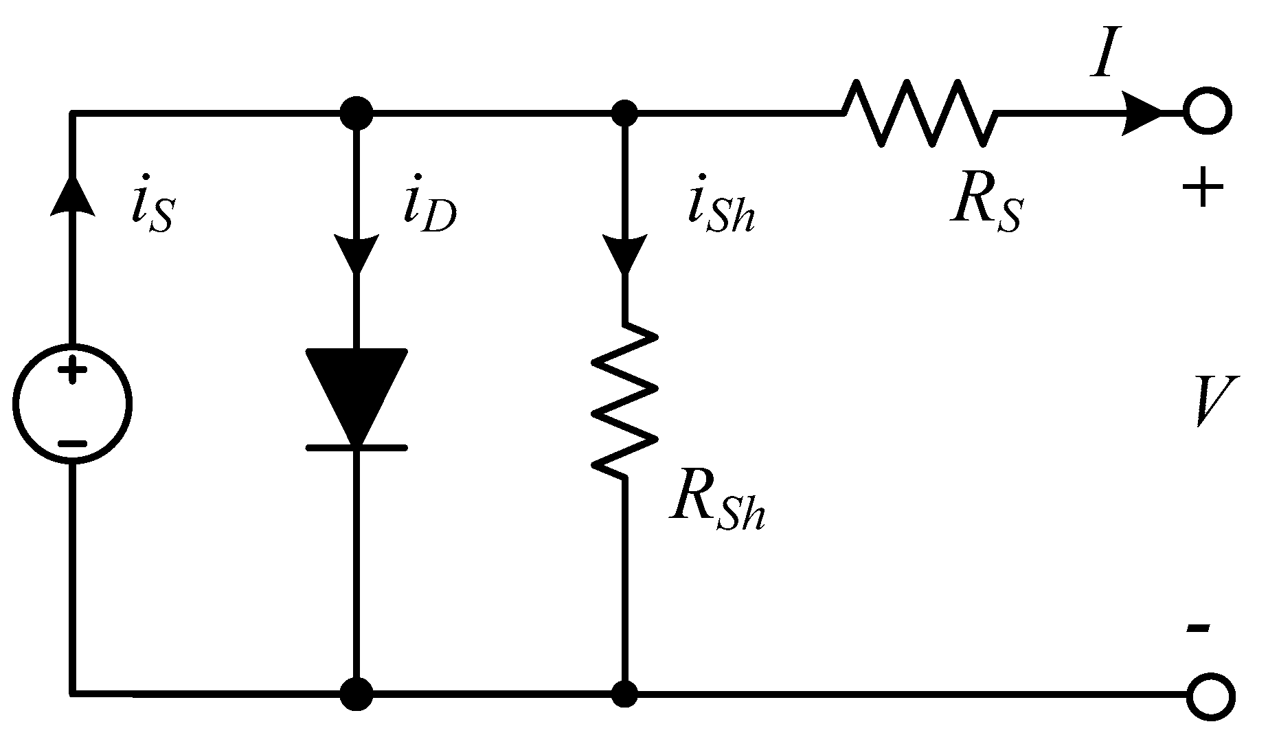
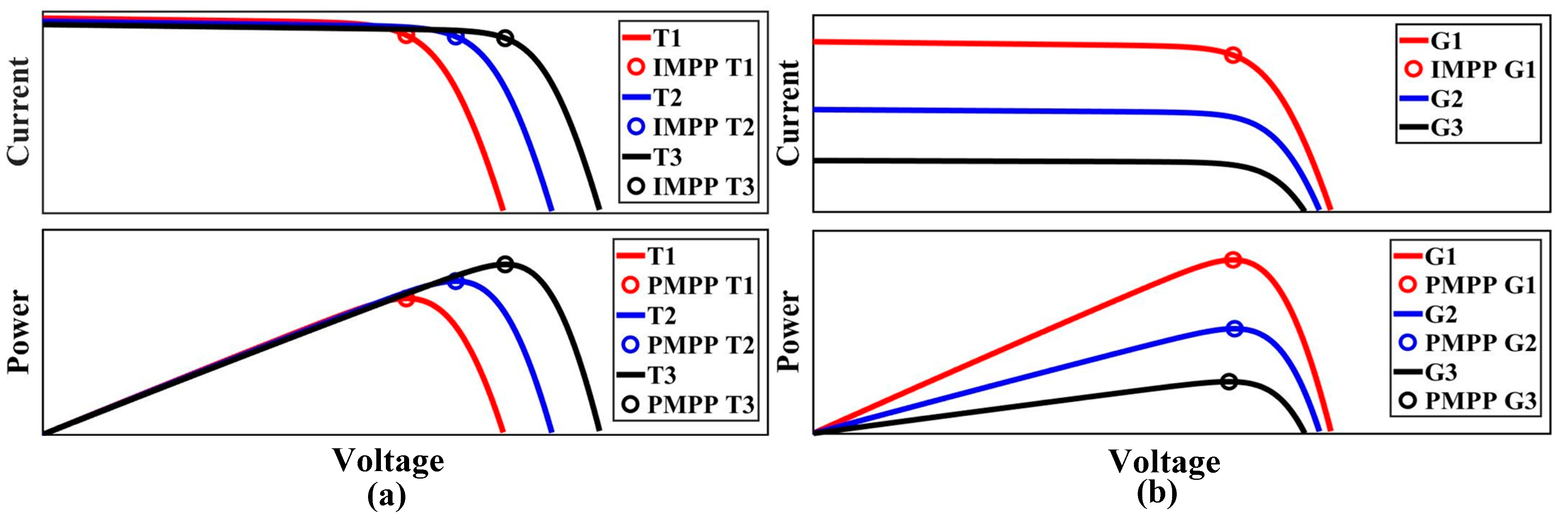
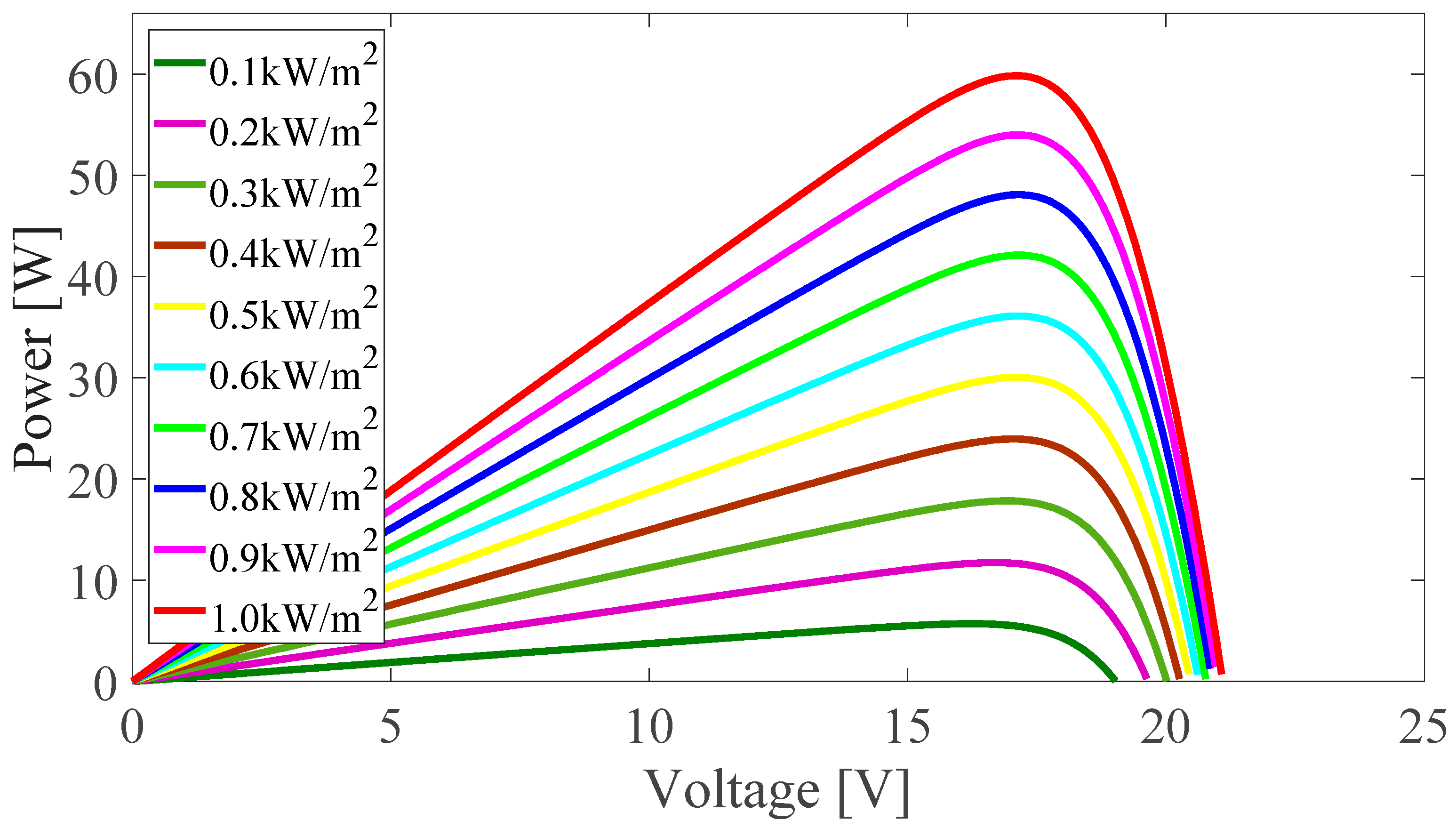
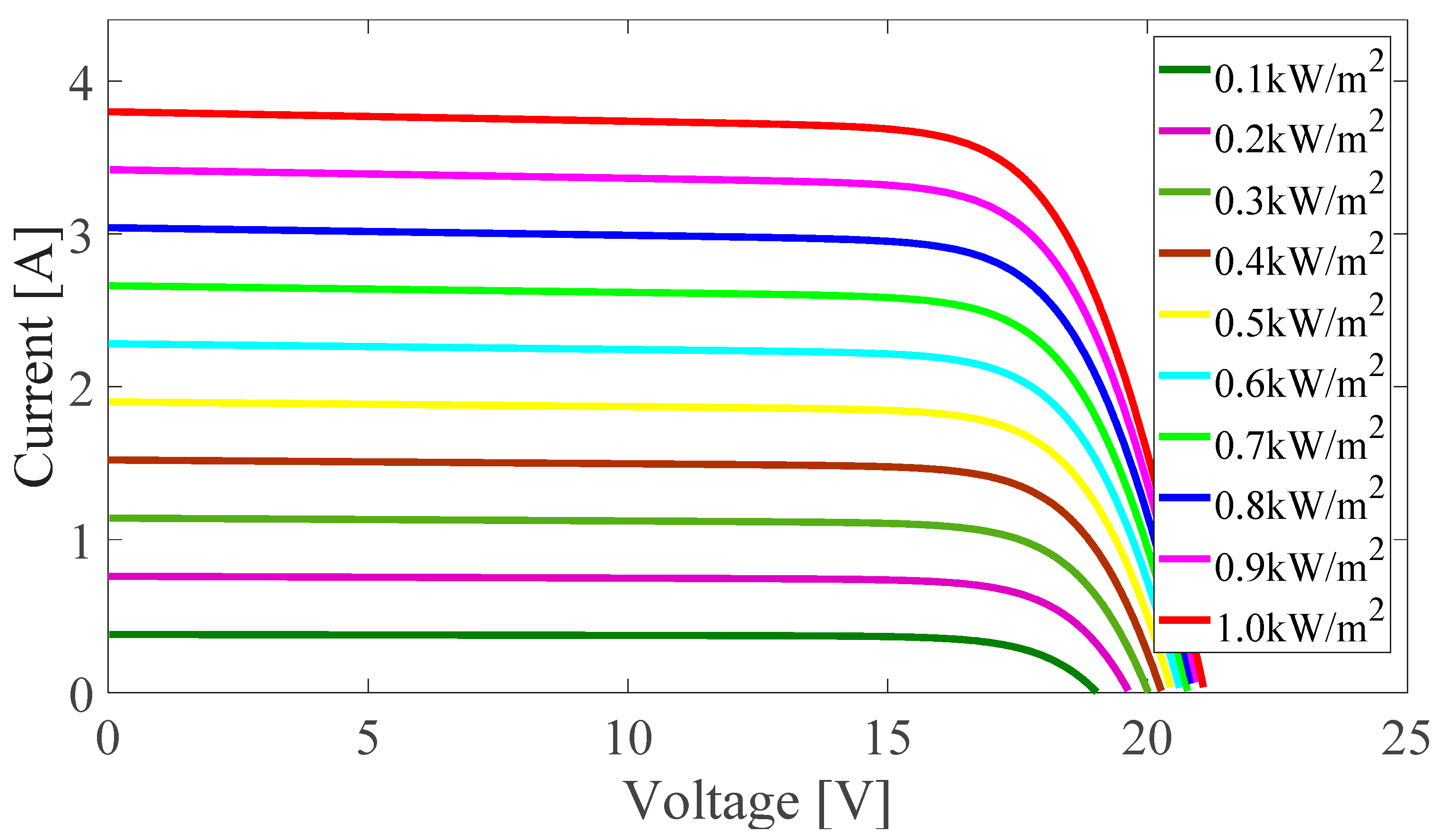
1.3. Model and Characteristics Analysis of PV Panel

The PV cell, also known as a solar cell, is the unit component of the PV panel and is a semiconductor device that can directly convert solar power into electrical energy based on the PV effect [34]. The irradiation directly affects the intensity of photocurrent generation, influencing the photovoltaics.
According to the one diode PV cell structure shown in Figure 2, a PV cell can be considered as the equivalent circuit depicted in Figure 2, consisting of an ideal current source (IL) with a diode (D), a series resistor (RS), and a parallel shunt resistor (RSh).
According to the equivalent circuit shown in Figure 2, the output current of a PV cell can be calculated as follows [6,26,35,36,37,38,39]:
I = I L I D I S h
Here, I is the output current (A), IL is the photocurrent (A), ID is the diode current (A), and ISh is the shunt current (A); IL, ID, and ISh can be expressed as follows [6,26,35,36,37,38,39].
I L = μ G
I D = I 0 { exp [ V + I R S n ( k q / T ) ] 1 }
I S h = V + I R S R S h
Here, μ is a proportional constant (depending on the material and other conditions), G is the illumination intensity, I0 is the diode reverse saturation current (unit: A), n is the diode ideality factor (1 < n < 2, and n = 1 for an ideal diode), k is Boltzmann’s constant (1.38 × 10⁻²³ J/K), q is the elementary electric charge e (1.6 × 10⁻¹⁹ C), T is the absolute surface temperature of the PV cell (unit: K), V is the output voltage, I is the output current (unit: A), RS is the series resistor (unit: Ω), and RSh is the shunt resistor (unit: Ω).
Combining Equations (2)–(4), as well as output current I, Equation (1) yields [6,26,35,36,37,38,39]:
I = μ G I 0 { exp [ q ( V + I R S ) n k T ] 1 } V + I R S R S h
According to Equation (5), the temperature and illumination intensity are the most influential environmental conditions in actual operation, because the other uncertain factors are confirmed upon the completion of the PV cell.
The characteristic current to voltage (I–V) and power to voltage (P–V) curves under different temperature and illumination conditions are shown in Figure 3. Changes in the temperature and illumination can easily affect the MPP, but in different ways. As shown in Figure 3a, under the same illumination (G), the increasing temperature (T) visibly reduces the output voltage of the PV panel, but the decrease in the output current is limited. This is followed by a decrease in the output power. As shown in Figure 3b, at the same surface temperature, as the illumination increases, the output voltage exhibits a slight increase, but the output current increases sharply, followed by an increase in the output power.

1.4. Maximum Power Point Tracking (MPPT)

The MPPT technique aims to maintain the maximum output operation of the PV system. MPPs in different environmental conditions are marked in Figure 3.
In most cases, a pulse-width modulation (PWM) wave is the control signal for the power switch of the converter; the duty cycle (D) of the PWM wave affects the output voltage, and an MPPT controller controls the duty cycle of the PWM wave [40,41].
In actual operation, the environmental conditions do not change sharply every second; nonetheless, the MPPT controller is needed to achieve the MPP. The core of the MPPT controller is the MPPT algorithm. According to their characteristics, MPPT algorithms can be classified into self-optimization and non-self-optimization algorithms. For example, perturb and observe (P&O) [29,40,42], incremental conductance (InC) [25,43,44], and constant voltage tracking (CVT) [40,45] are three typical self-optimization algorithms. Non-self-optimization algorithms mainly include curve fitting [46] and other methods. Furthermore, there are artificial intelligence techniques, such as fuzzy logic [12,47,48] and particle swarm optimization [12,49,50,51,52], that are combined with conventional MPPT methods to achieve a high tracking accuracy.
In the industry, MPPT controllers, mostly self-optimization-based, can help systems track the MPP and automatically maintain steady operation in the maximum-output state. A comparison of three typical methods is shown in Table 1. After the comparison, to simplify the algorithm, the proposed MPPT algorithm is P&O-based [29,42,53], and its differences from the conventional one [13,16,30,36,45,46,53] are introduced in the Methods section of this report.

2. Methods

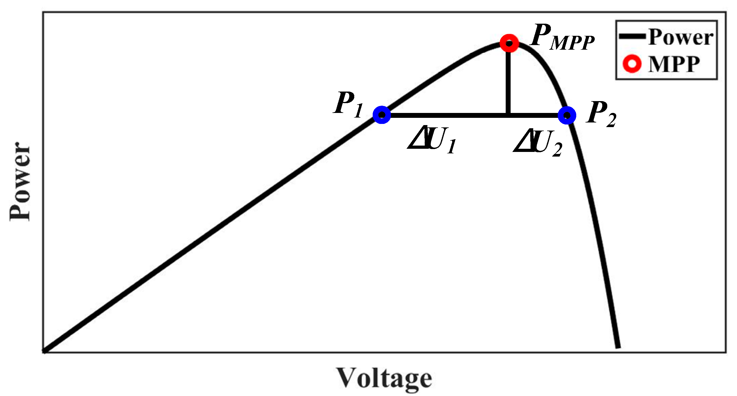
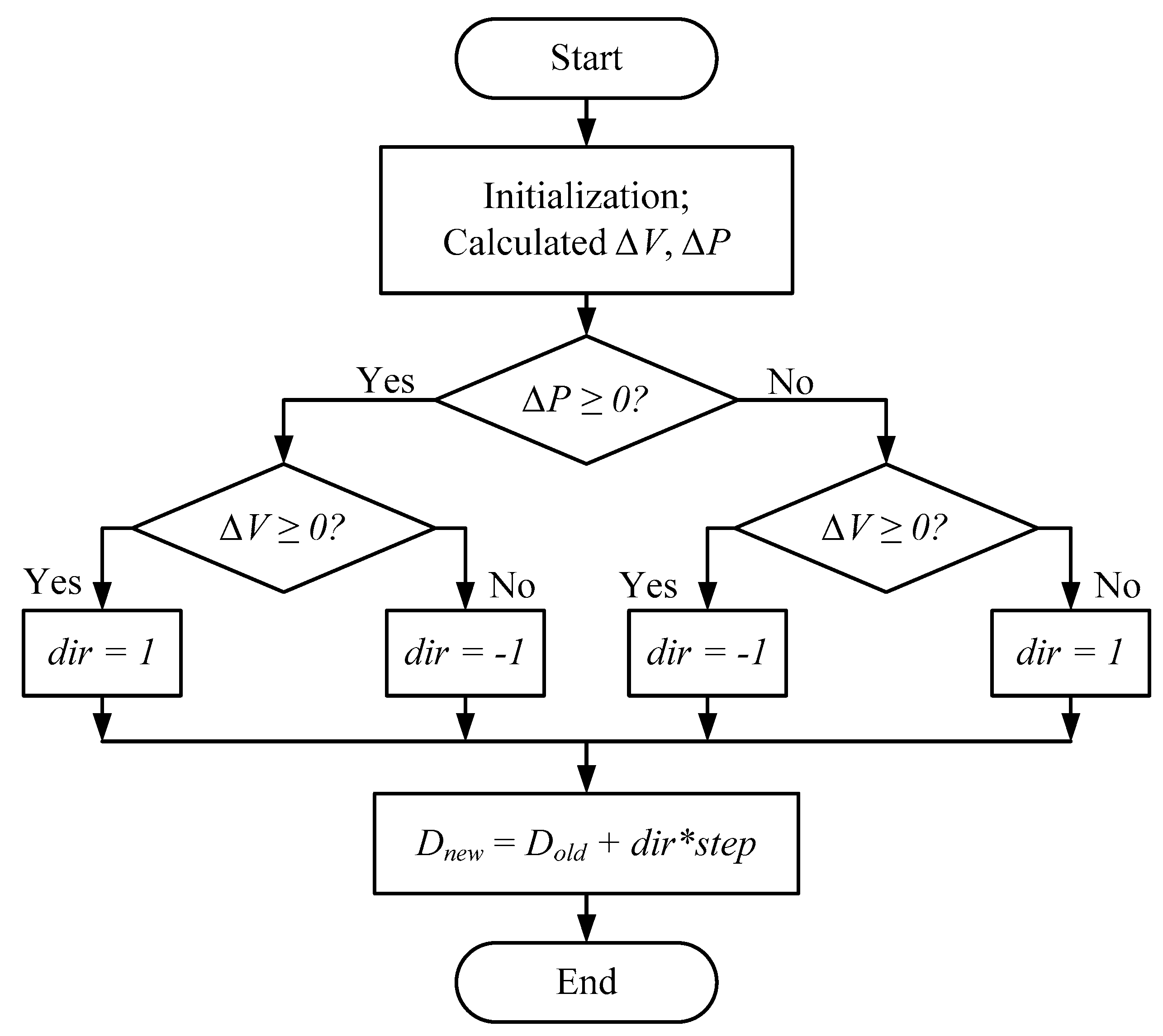
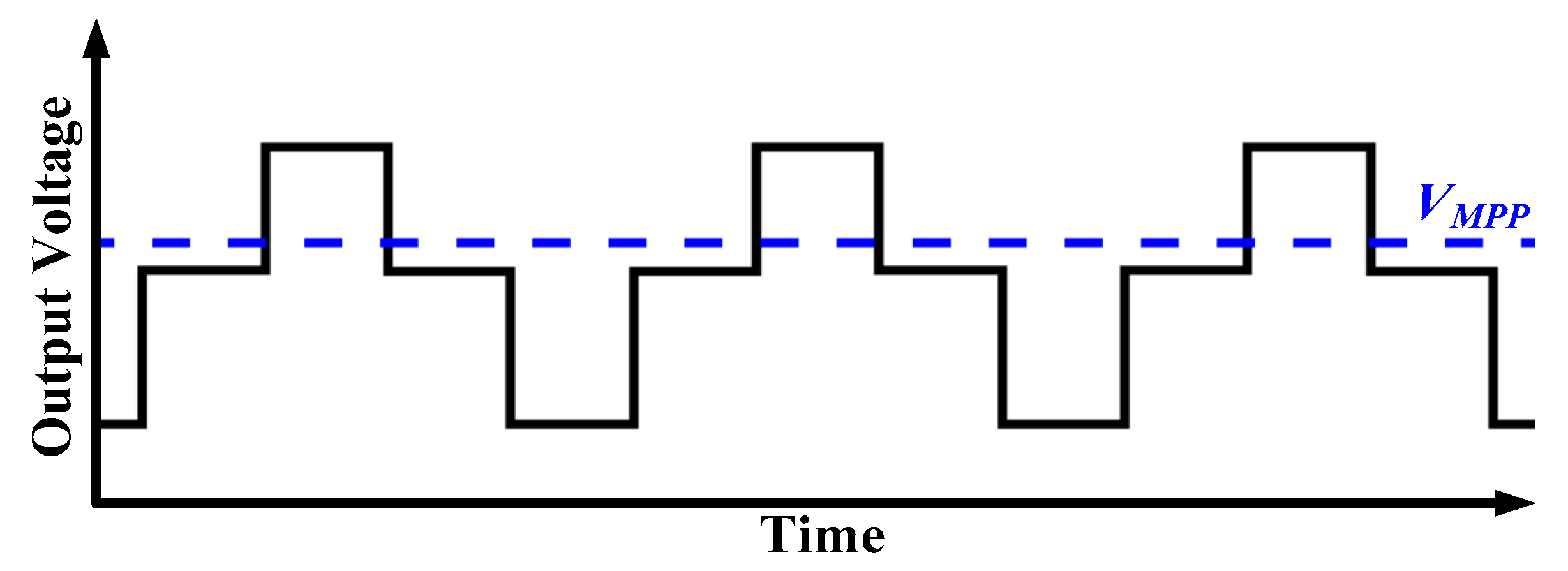
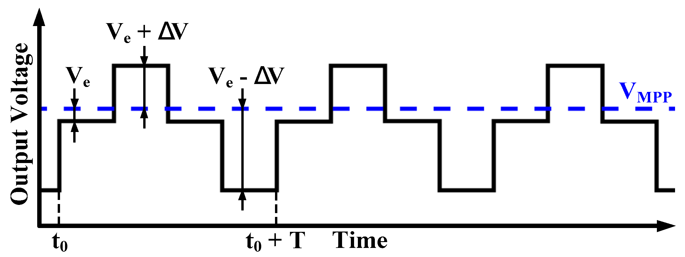
2.1. Principle of the P&O Method

The P&O method is the most widely used self-optimization MPPT algorithm. The basic principle of P&O is as follows. After a certain directional-changing voltage applies perturbation to the output voltage of the PV panel, the MPPT controller compares the output power before and after the perturbation. If the changing direction is positive and the output voltage increases, the MPPT controller continues the perturbation in this direction; if the output power decreases, the direction reverses in the next perturbation.
Figure 4 shows the characteristic P–V curve, where PMPP is the MPP, P1 is to the left of the MPP, P2 is to the right of the MPP, and ∆U1 and ∆U2 are the changing ranges of the output voltage. To achieve the MPP, ∆U1 should be increased in P1, but ∆U2 should be decreased in P2. In this case, ∆U1 and ∆U2 differ, and ∆U1 > ∆U2. A greater distance from the MPP yields a greater difference between ∆U1 and ∆U2. Owing to the existence of perturbation, it is very difficult for the basic P&O method to eliminate the oscillating phenomenon at the MPP. The step size of the perturbation directly affects the speed and accuracy of the MPPT. All of these factors cause power loss. Figure 5 [40] presents the flowchart of the basic P&O tactic.

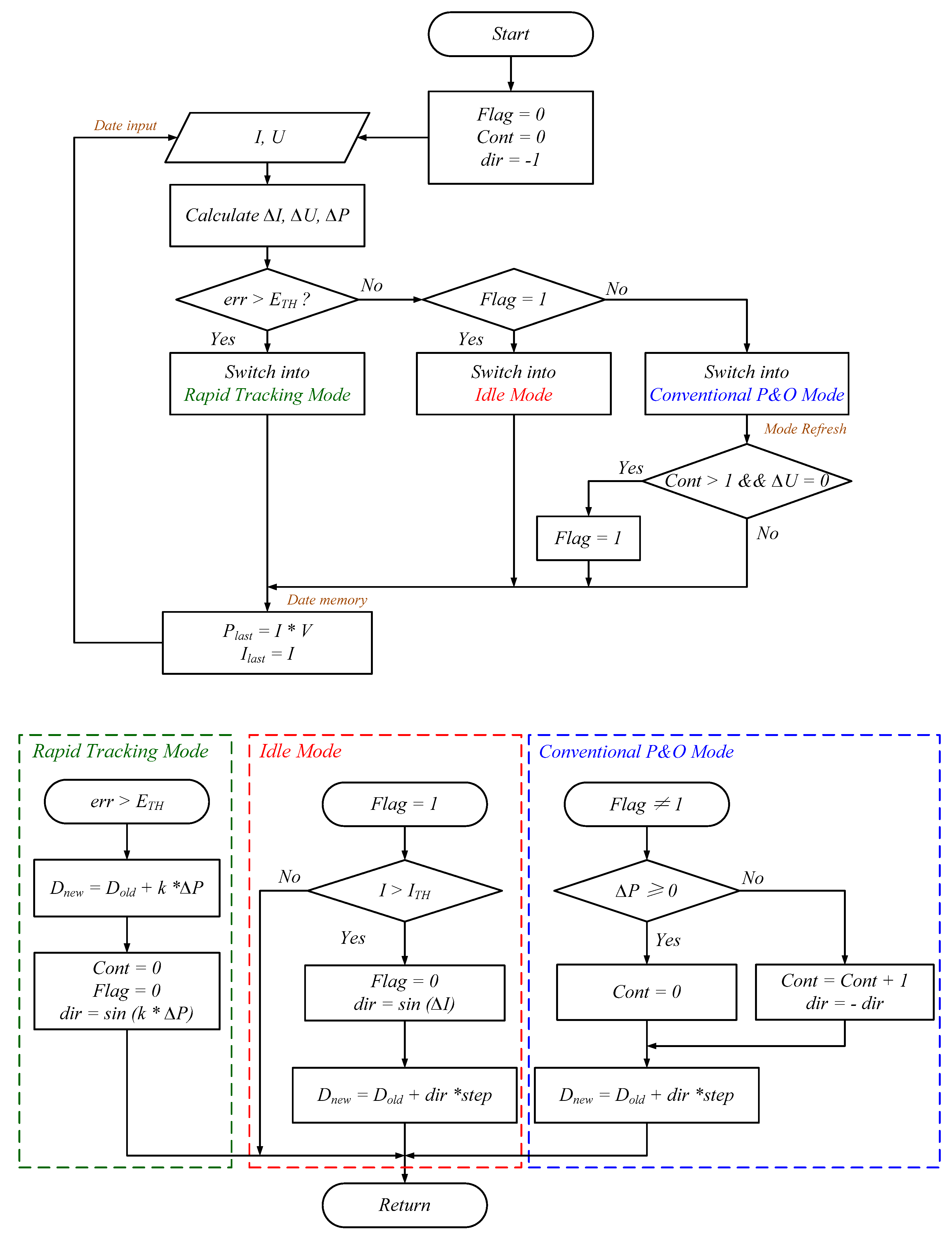
2.2. P&O-Based Self-Adaptable Step Size MPPT Tactic

In the case of a fixed step size P&O algorithm, opportunely increasing the step size can improve the system response speed, but increase the oscillation region around the MPP and increase the power loss. A small step size can increase the tracking accuracy and reduce the oscillation, but reduce the response speed. To deal with the contradiction between accuracy and response speed, the variable step size MPPT algorithm is employed. The conventional variable step size MPPT algorithm comprises the optimum gradient method [23,54], the successive approximation optimization method [29,30,42,43,55], and other methods. However, the derivative of the power to the voltage is too large on the right side of the MPP; therefore, the derivative of the power to the voltage is no longer suitable for the parameter of the step size solution. However, the optimal gradient-based variable step size MPPT uses a stationary step size selection equation; this algorithm cannot preferably adapt to changes in the P–V curve.
The tracking tactic of the conventional MPPT algorithm is periodic. For the conventional P&O strategy, the step size is fixed, which means that the ∆U in the operating procedure, shown in Figure 5, cannot change. Owing to the tracking issues presented in Figure 4, a certain oscillation exists. Because of the aforementioned issues, in the steady operation state, although the MPPT controller has tracked the MPP successfully, the output voltage still undergoes perturbation around the MPP and never achieves VMPP (output voltage in the MPP), as shown in Figure 6, and the exiting oscillation around the MPP causes certain power loss. The definition and analysis are introduced in the power-loss analysis and calculation part of this report. To deal with the power loss around the MPP in the steady-state operation as much as possible, an advanced P&O-based MPPT tactic with a self-adaptable step size is proposed. A flowchart of the proposed MPPT tactic is presented in Figure 7.
Compared with the conventional P&O MPPT [29,30,40,42], the improved procedure of the proposed P&O-based self-adaptable MPPT tactic is based on the following four key aspects: (1) natural oscillation control, (2) system operation state determination, (3) perturbation direction decision, and (4) adaptable step size.
In the natural oscillation control procedure, the proposed tactic can select a suitable tracking loop depending on the oscillation range. In the flowchart, P and err detects the output power change in present and previous sample period; ETH is the threshold for error determination. It is used to control the allowable natural oscillation range and as an entry for a continuous module. If err > ETH, the program uses the error value and multiplies it by a weight factor (k) as the step size to optimize the tracking speed; otherwise, the program enters the system operation state determination module.
In the system operation state determination module, Flag is the identifier of the operation state. If Flag = 1, the tracking procedure enters an idle operation loop, and the next perturbation director (dir) depends on whether the actual current (I) reaches the threshold for current (ITH), expressed in Equation (7). If ∆I > ITH, Idle changes to 0, and the direction (dir) is a sine function of ∆I and is the weight of the next perturbation; or, it jumps out of the Idle Mode loop. If Idle = 0, the program enters the P&O-based perturbation direction decision procedure.
The procedure of perturbation direction decision is similar to the operation of the basic P&O tactic, but differences exist. The direction for the next perturbation depends on the change in the output power (∆P). If the output power in this perturbation is increased (∆P > 0), the perturbation direction is continuous, and the counter is initialized (Cont = 0); otherwise, the perturbation direction is changed (dir = −dir), and the loop time is counted (Cont = Cont + 1). After the conventional P&O procedure, the program determines the change in the output voltage (∆U) and the number of loop times (Cont). If it loops more than once (Cont > 1) and the change in the output voltage is null (∆U = 0), the program operates in the Idle mode (Flag = 1), provided that the error is within the allowable range.
As shown in Figure 6, the standard P&O tactic gives rise to a certain oscillation around the MPP, and the range of the oscillation depends on the setting of the perturbation step size. The adaptable step size is included in every aspect introduced above. Mainly, the step size depends on the change in the last operation state (Flag = 0 or Flag = 1) and the range of actual oscillation (err). The change in the step size affects the duty cycle of the PWM wave and is displayed as the change in the output voltage of the boost converter. In this tactic, the step size is identified as step and can be measured by determining the output voltage or duty cycle of the PWM wave in actual operation.
The boundary condition chosen is based on the characteristics of selected PV elements as shown in Table 2. During the irradiation change, the change in interface temperature would not be significant. Hence, the consideration of boundary selection is only based on the change in MPP while the irradiation changes.
In the simulation, the boundary condition of ETH is selected by the change in measure power during the no-oscillation state. The value of ETH is selected as 0.03; in other words, the judgement follows the relationship of |(P-P_old)/P_old| >= 0.03 (P is the present sampled power and P_old is the value in previous sample time). |(P-P_old)/P_old| is the explaination for err. The selection of 0.03 is based on the change in power while the irradiation changes for the PV element MSX-60W, as shown in Figure 8. According to Figure 8, if the change in power is more than 0.03 of the previous MPP point, the change in irradiation could be determined and the Rapid Tracking Model is activated.
The selected of ITH in the Idle Mode is based on the change of MPP current in the MPP region, as shown in Figure 9. At the MPP, the relational gain KIsc between MPP current Impp and short-circuit current Isc is a constant, and 0.78 < KIsc < 0.92 [56]. In this condition, the Isc can be estimated using the listing formula in the left of the MPP.
I s c = I I I _ o l d V V _ o l d · V
KIsc is selected as 0.92 in the simulation.
ITH is expressed as follows:
I T H = K I s c ( I I I _ o l d V V _ o l d · V )

2.3. Simulation Modeling and Power-Loss Analysis

In this part, the simulation modeling and the mathematical method for the power-loss analysis are introduced. To verify the proposed MPPT tactic, a MATLAB/Simulink module is used as a platform for simulation. During the simulation, some parameters are changed to simulate the change in the environmental conditions. The power-loss analysis and calculation are expressed by mathematical equations.

2.4. Simulation Modeling

Simulation modeling mainly includes three key aspects: (1) PV module modeling, (2) MPPT controller modeling, and (3) PV system combination. The modeling strategies and parameter settings are presented in the tables and figures.

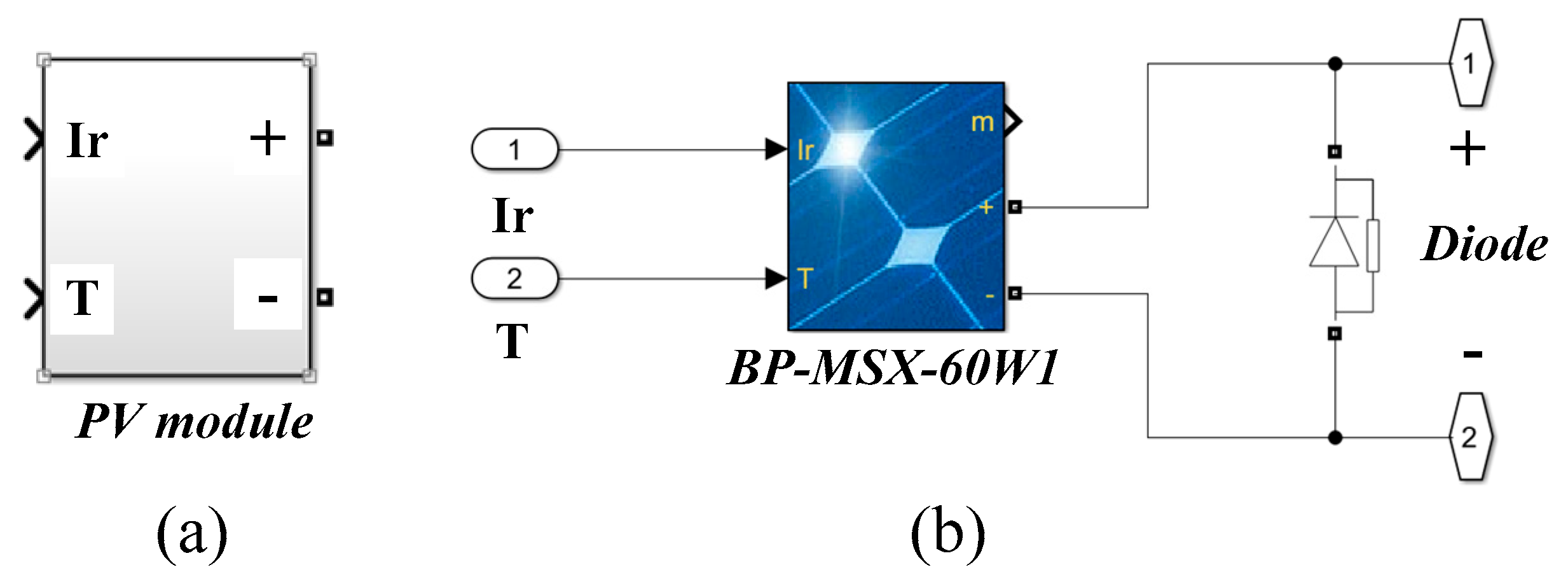
2.4.1. PV Module Modeling

The modeling of the PV array module is based on the template BP MSX-60W1 from Simulink Library. The symbol and connection are displayed in Figure 10, and the parameters are explained in Table 2.
In Figure 10, Ir is the input for the illumination intendancy, T is the input for the temperature, “+” is the positive electrode of the output voltage, and “−” is the negative electrode of the output voltage. The diode in Figure 10b protects the PV panel.
In Table 2, N is the number of cells per module, PMPP is the maximum power, VOC is the open-circuit voltage, VMPP is the voltage at the MPP, ISC is the short-circuit current, IMPP is the current at the MPP, CVOC is the temperature coefficient of VOC, and CISC is the temperature coefficient of ISC.

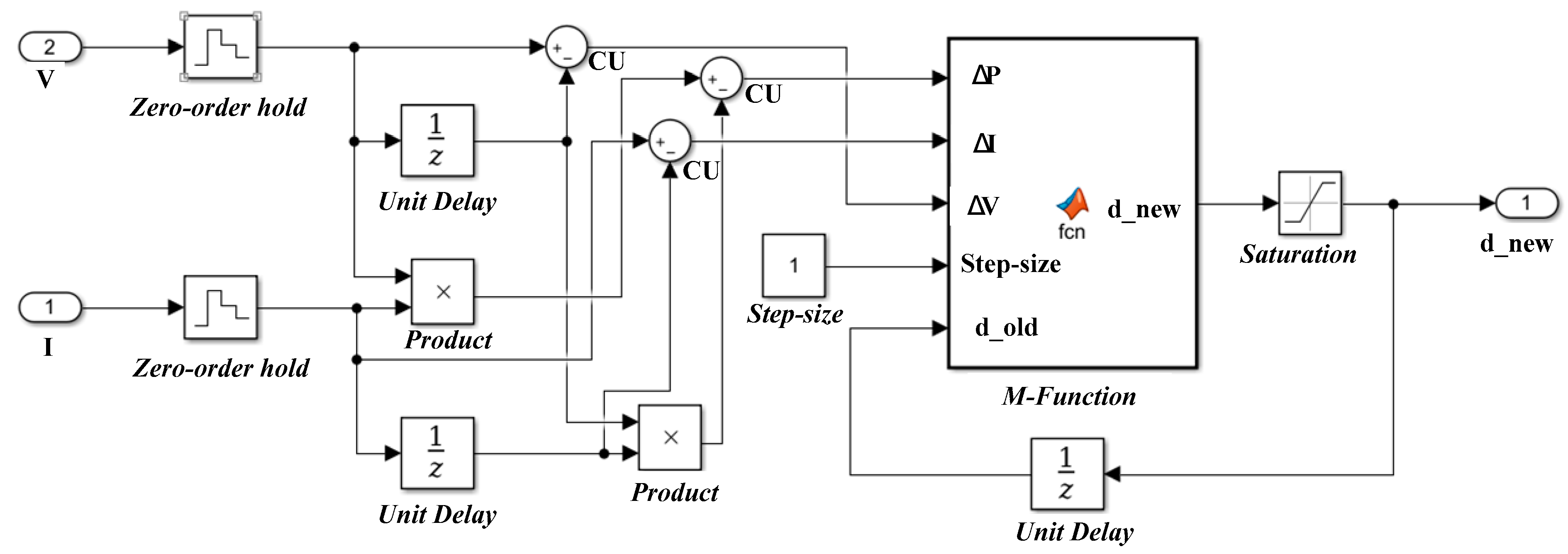
2.4.2. MPPT Controller Module Modeling

To compare the conventional and proposed MPPT tactics, two MPPT controller modules were built. Figure 11 shows the connections of the proposed MPPT control. The codes in the m-functions are based on the flowcharts shown in Figure 7.
In Figure 11, V is the input data of voltage, I is the input data of current, “zero-order hold” is for updating and holding data at every sample time, “unit delay” is for memorizing data, “product” is a multiplier, “CU” is the unit for data minus, “step size” is for setting the initial value of the step size, “M-function” is a function builder that employs the m-language (five input ports: three for the change in power, current, and voltage; one for initial step size setting; and one for the old duty cycle), “saturation” is for limiting the upper and lower values of a signal, and “d_new” is the updating duty cycle of the PWM wave.

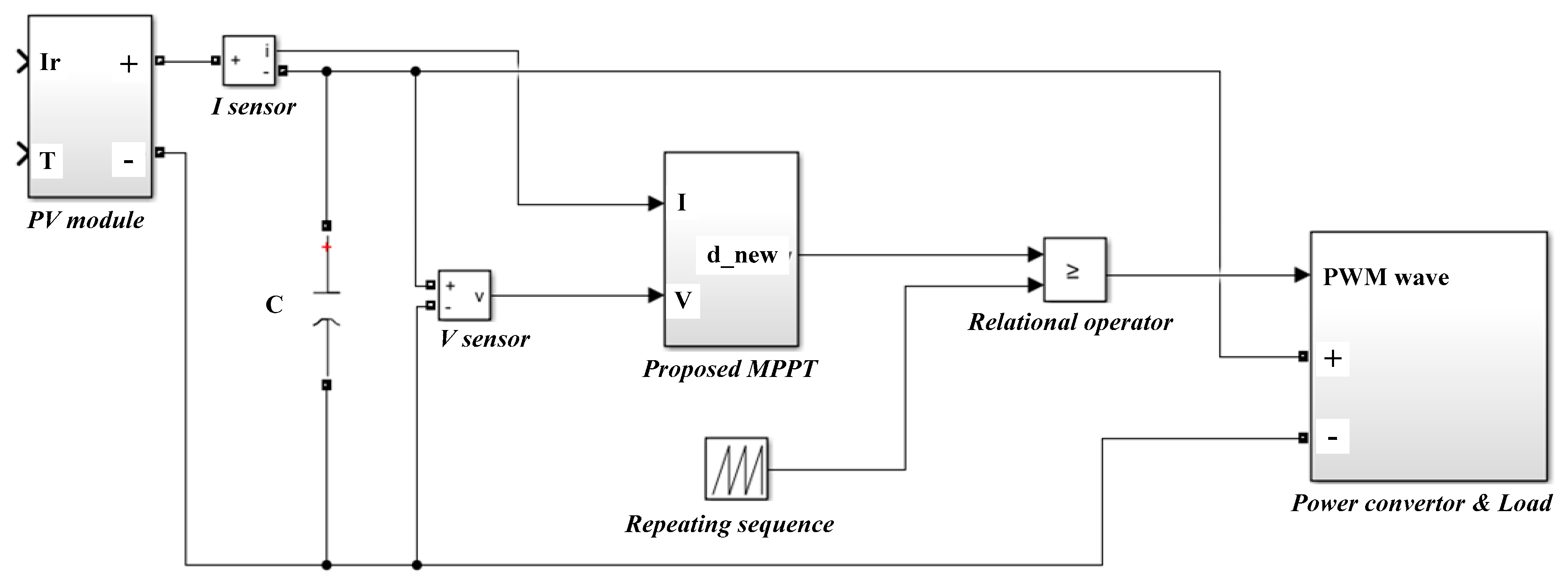
2.4.3. PV System Combination

According to the basic structure of the PV system displayed in Figure 1, the proposed P&O-based PV system simulation platform is shown in Figure 12.
The PV module is introduced in the PV array modeling section. The proposed MPPT is explained in the Methods section, and the initial connection is shown in Figure 12. The power converter and load include a boost converter and a 30-Ω resistor (as the electrical appliance); Ir is an input port for the illumination, T is an input port for the temperature, the I sensor is for measuring the photocurrent, the V sensor is for measuring the photovoltage, and C is a filter capacitor (47 μF). The repeating sequence and relational operator work together and generate the control signal (PWM wave) for the power converter. The connections are based on the initial characteristics of each component.

2.5. Power-Loss Analysis and Calculation

The power-loss analysis is an important aspect for defining the tracking efficiency of the MPPT. The artificial oscillation around the MPP of the proposed MPPT strategy is diminished to close to zero and can even be removed in an ideal environment; moreover, the tracking step size can be adapted automatically. A typical operation issue of the conventional P&O MPPT strategy is displayed in Figure 13, and the power-loss analysis and calculation are based on this figure.
The relationship between the power loss (PL) and the theoretical power (PMPP) is expressed as follows [57]:
P L P M P P ( ( Δ V P V ) R M S V M P P ) 2 ( 1 + V c e l l 2 n k T / q )
Here, VMPP is the theoretical output voltage when the PV panel operates in the MPP, (∆VPV)RMS is the root-mean-square [58] value of the voltage perturbation, and Vcell is the output voltage of every single cell when the PV panel operates in the MPP (mostly around 0.5 V).
According to Figure 13, in one oscillation cycle (T), the function of the change in the output voltage corresponding to time (∆VPV(t)) is expressed as follows.
Δ V P V ( t ) = { V e ( t 0 < t < t 0 + T / 4 ) V e + V s t e p s i z e ( t 0 + T / 4 < t < t 0 + T / 2 ) V e ( t 0 + T / 2 < t < t 0 + 3 T / 4 ) V e V s t e p s i z e ( t 0 + 3 T / 4 < t < t 0 + T )
Here, Ve is the minimum difference between VMPP and the output voltage (VPV ) set by the MPPT controller, and Vstep size is due to the step size and is displayed as ∆V in Figure 12. The relationship between Ve and Vstep size can be observed as follows.
V e = β V s t e p s i z e
Here, β is a constant. Replacing Ve with Equation (9), Equation (10) can be expressed as follows.
Δ V P V ( t ) = { β V s t e p s i z e ( t 0 < t < t 0 + T / 4 ) ( β + 1 ) V s t e p s i z e ( t 0 + T / 4 < t < t 0 + T / 2 ) β V s t e p s i z e ( t 0 + T / 2 < t < t 0 + 3 T / 4 ) ( β 1 ) V s t e p s i z e ( t 0 + 3 T / 4 < t < t 0 + T )
Therefore, the root-mean-square (RMS) value of the voltage perturbation ((∆VPV)RMS) can be calculated as follows.
( Δ V P V ) R M S = 1 T 0 T Δ V t 2 d t = V s t e p s i z e 1 4 ( β 2 + ( β + 1 ) 2 + β 2 + ( β 1 ) 2 ) = V s t e p s i z e 1 2 + β 2
By combining Equations (8) and (12), the steady-state power loss can be expressed as follows.
P L P M P P ( 1 2 + β 2 ) ( V s t e p s i z e V M P P ) 2 ( 1 + V c e l l 2 n k T / q )
For the proposed MPPT tactic, the output voltage does not give rise to any artificial oscillation, but differences still exist between VPV and VMPP. The difference between VPV and VMPP in this condition can be expressed as follows.
( Δ V P V ) R M S = β V s t e p s i z e
By substituting Equation (14) into Equation (8), the power loss of the proposed MPPT tactic can be expressed as follows.
( P L P M P P ) p r o p o s e d β 2 ( V s t e p s i z e V M P P ) 2 ( 1 + V c e l l 2 n k T / q )

3. Results and Discussion

The results are categorized into two parts: (1) the simulation results are displayed, analyzed, and compared with the conventional P&O MPPT tactic to show the improvement; and (2) the power loss is calculated via the statistical method expressed in the Methods and power-loss analysis and calculation parts of this report.

3.1. Simulation Results

To verify the advanced performances of the proposed MPPT controlling tactic, the simulations follow the single-variable principle, and the comparisons are performed under the same parameter settings (excluding the MPPT controller module). The settings of the PV array module and the other basic simulation parameters are shown in Table 3.
The simulation results are divided into three parts: (1) tracking speed comparison under steady environment conditions, (2) reliability under variable environment operation, and (3) improvement of the steady state operation.

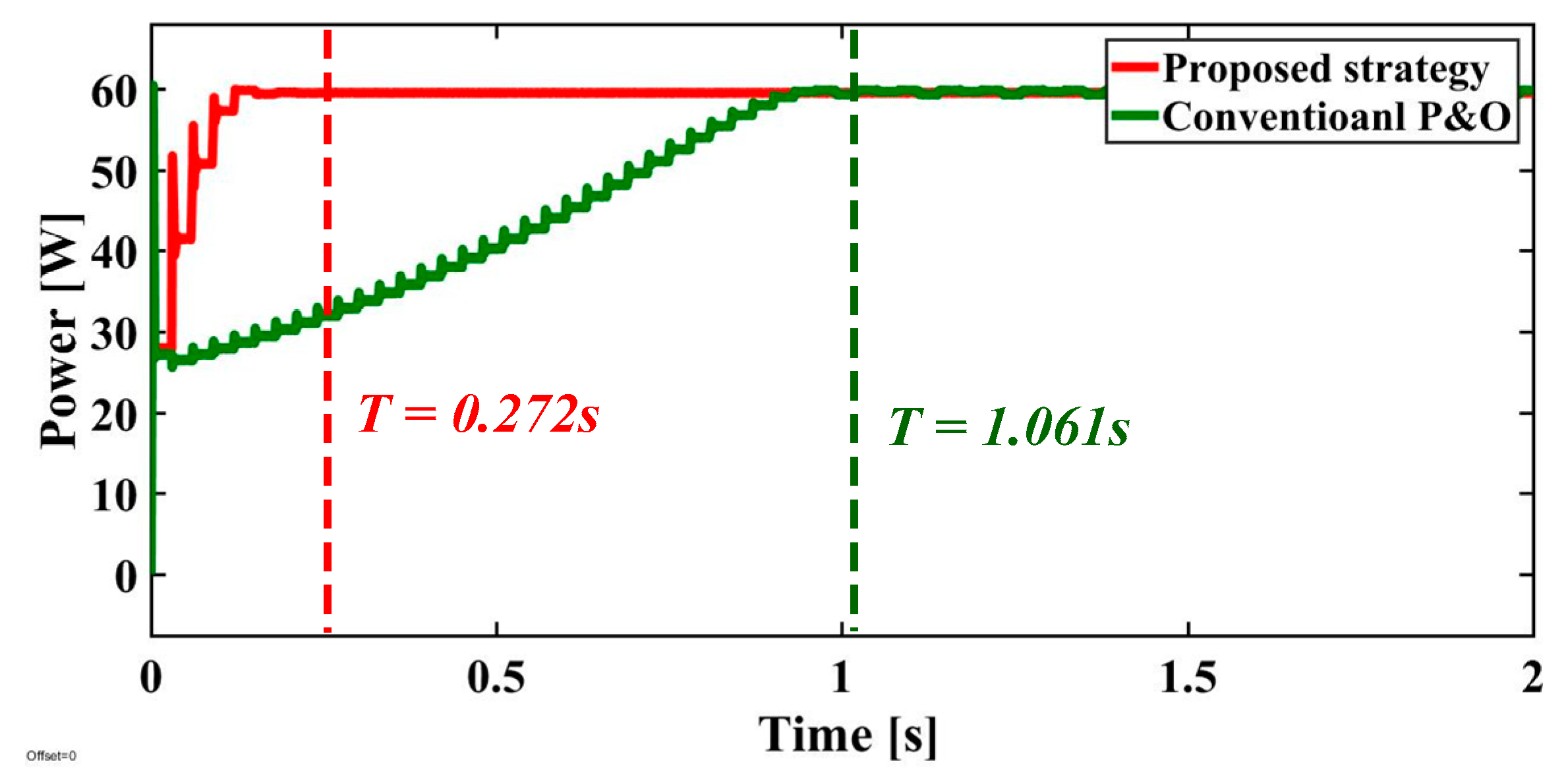
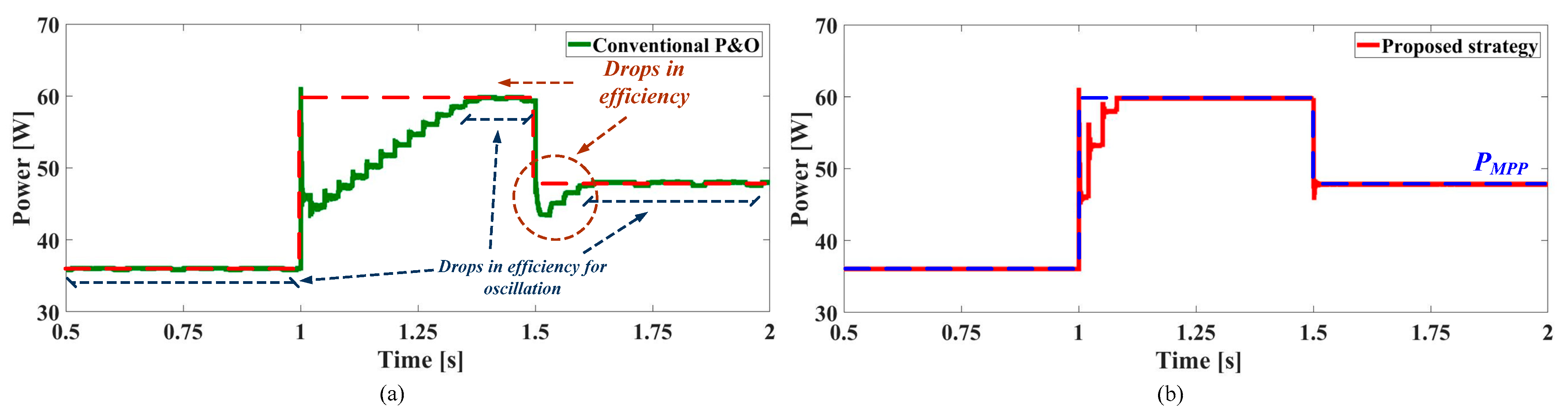
3.1.1. Tracking Speed Comparison

The simulation verifies the increasing tracking speed of the proposed MPPT tactic. The other simulation parameter is set to the ideal value (illumination = 1000 W/m2) to eliminate the effects of environmental conditions.
Figure 14 shows the power–time curves of the proposed MPPT tactic (red line) and the conventional P&O algorithm (green line). According to Figure 14, the time needed for the conventional P&O MPPT tactic is 1.061 s, and that for the proposed MPPT tactic is 0.272 s. The decrease in the tracking time verified the increase in the tracking speed; compared with the conventional P&O tactic, the proposed tactic can reduce the tracking speed by approximately 74.5%.

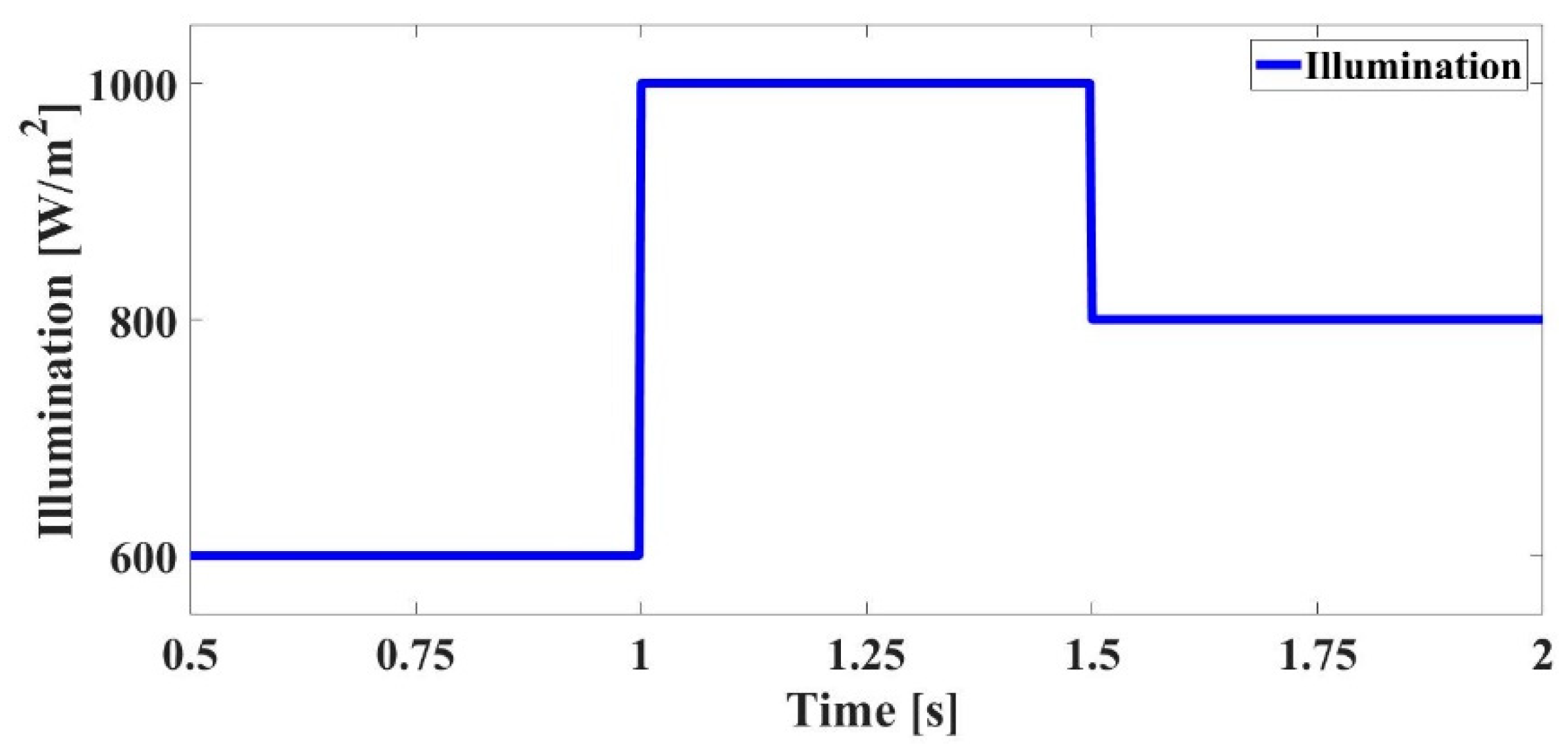
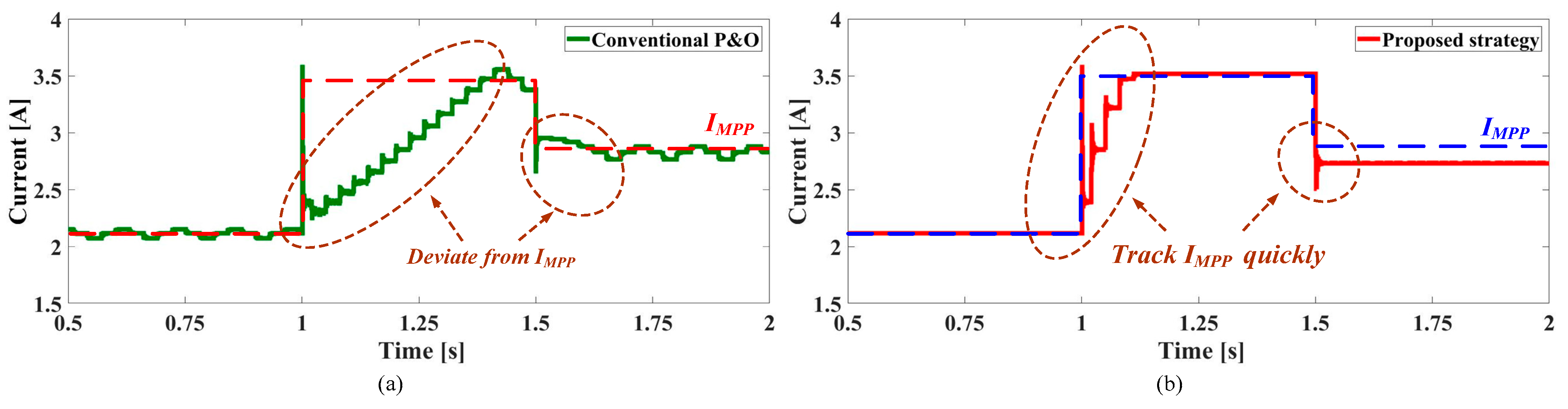
3.1.2. Reliability under Variable Environmental Conditions

In actual operation, the change in temperature is not sharp, and the main influencing factor is the change in illumination because of partial shading; therefore, the reliability of the proposed tactic is defined via simulation in the environment with a variable change in illumination, as shown in Figure 15.
In this situation, the simulation results, including the current, voltage, and power curves, are shown in Figure 16, Figure 17 and Figure 18, respectively. In these figures, short explanations of the existing phenomenon are presented. Each figure includes two parts—one is from the conventional P&O tactic, and the other is from the proposed MPPT tactic. Each sub-figure has a standard line of the theoretical output parameters in MPP operation for verifying the tracking accuracy.
Figure 16 shows the curves of the PV array output current (IPV). Figure 16a shows the measured current for the conventional P&O tactic. The results for the tracking during the increase in the illumination show a lack of speed and departures from the standard line (IMPP). As shown in Figure 16b, the proposed tactic does not cause departures and has a high tracking accuracy with the standard.
Figure 17 shows the curves of the PV array output voltage (VPV). The conventional P&O tactic can track the MPP, but a loss of efficiency exists in the illumination increasing procedure. This method tracks in the wrong direction owing to the falling illumination and returns to the right direction when this phenomenon stops. During the increase or decrease in the illumination, the proposed strategy operates in the self-adapted step size model and maintains a limited departure from the theoretical output voltage.
Figure 18 shows the curves of the PV array output power (PPV). According to the tracking mistakes and errors, the conventional tactic results in efficiency drops, as shown in Figure 18a. At the same time, the oscillation around the MPP causes efficiency drops. As shown in Figure 18b, the output–power curve of the proposed tactic almost coincides with the theoretical output of that of a verification of the tracking accuracy and efficiency.

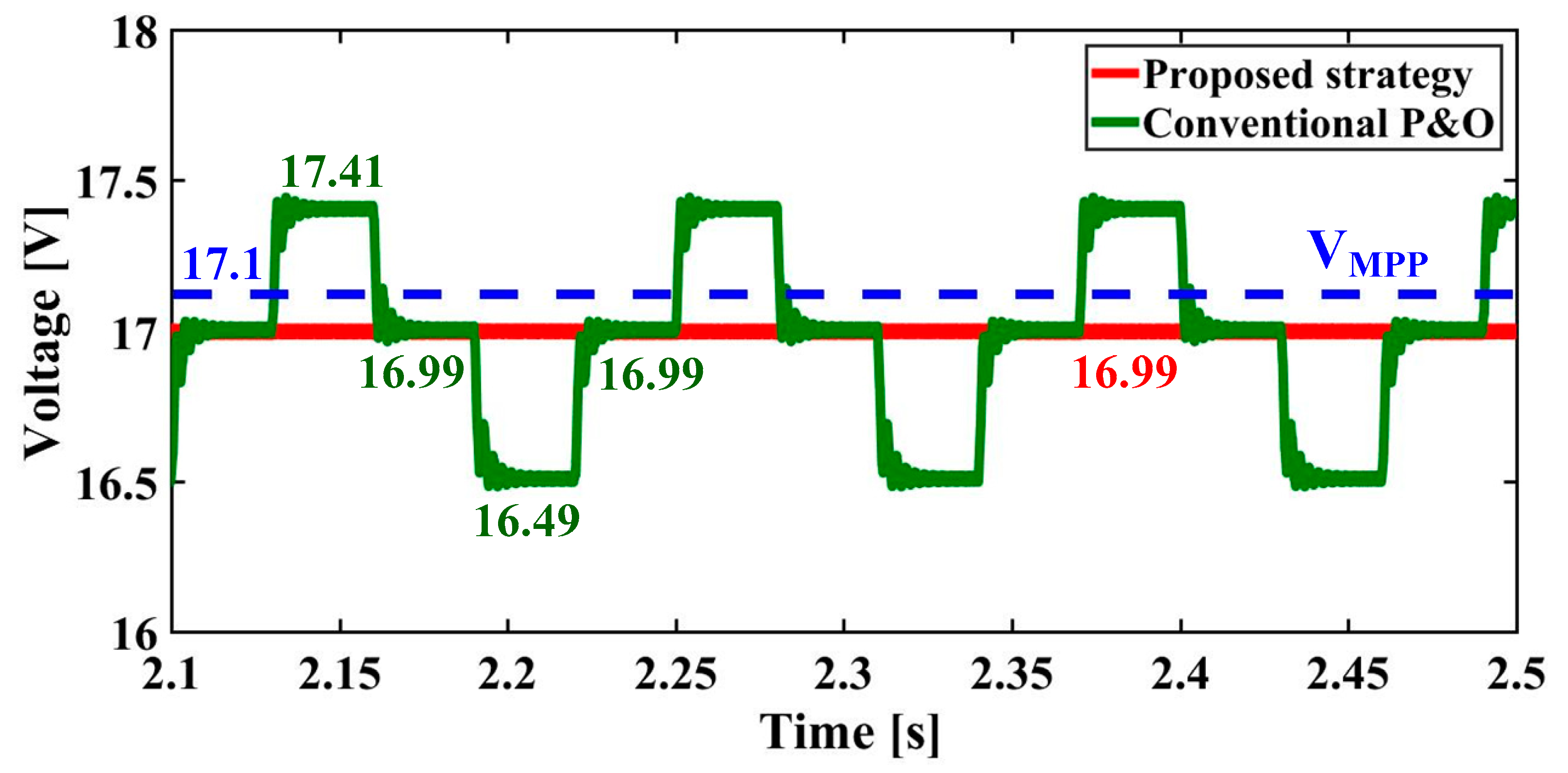
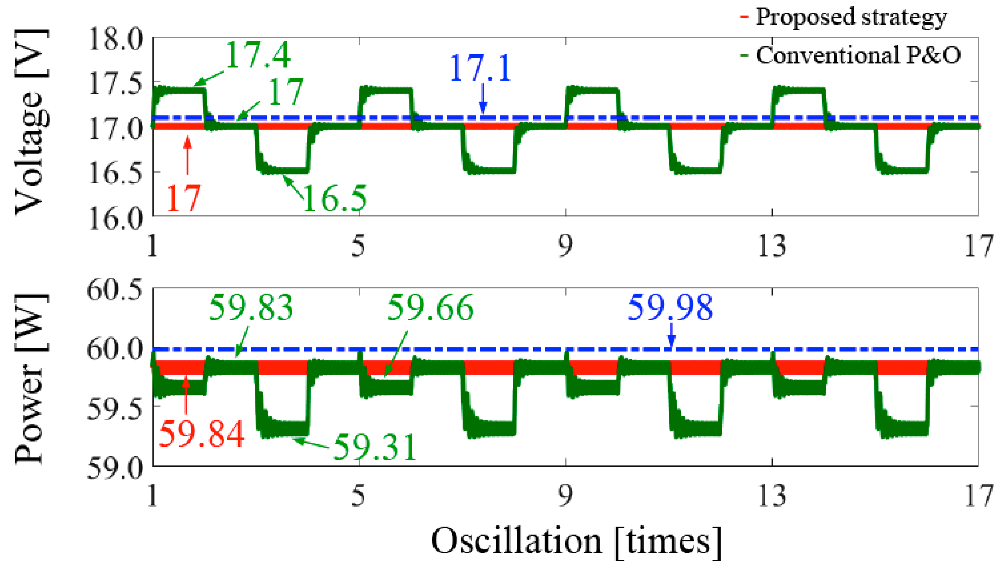
3.1.3. Steady-State Operation Comparison

Figure 19 shows the output–voltage state under steady operation. Compared with the theoretical output value (VMPP), there exist conventional P&O strategy oscillations around the MPP in the steady state; the proposed tactic experiences deviations from the theoretical output, but can maintain operation without oscillation.

3.2. Power-Loss Analysis Results

According to Figure 19 and the parameters of the PV module shown in Table 2, the power loss can be calculated using the equation expressed in the Methods section of this report.
According to Equations (8) and (11), the steady-state power loss of the conventional P&O tactic is calculated as follows.
( P L P M P P ) c o n v e n t i a n l 0.69 %
According to Equations (8) and (13), the steady-state power loss of the conventional P&O tactic is given as follows.
( P L P M P P ) p r o p o s e d 0.23 %
The efficiency of the power-loss reduction is calculated as follows.
η e f f i c i e n c y = ( 1 0.23 % 0.69 % ) × 100 % 66.7 %
Via the proposed strategy, the power loss in steady-state operation drops to 0.23%; compared with the conventional P&O algorithm, the percentage reduction in the power loss around the MPP is 66.7%.
Assuming the PV element is in the standard test condition (STC) (1000 W/m2, 25 °C, AM1.5), the simulation in steady-state operation for the conventional P&O MPPT and proposed control is as shown in Figure 20.
The percentage of power absorbed in every oscillation period for the conventional P&O algorithm can be calculated as follows.
P t 1 + P t 2 + P t 3 + P t 4 P t h e o = 59.66 W + 59.83 W + 59.31 W + 59.83 W 59.98 W × 4 × 100 % = 99.46 %
where Pti is the ith oscillation in a period and Ptheo is the theoretical output power during the period.
The power absorbed in every oscillation period for the proposed control scheme can be calculated as follows.
P t 1 + P t 2 + P t 3 + P t 4 P t h e o = 59.84 × 4 59.98 W × 4 × 100 % = 99.77 %
The power loss in the P&O algorithm is expressed as 0.54% and 0.23% for the proposed control. The simulation result is close to the calculation in the submitted manuscript. The energy saving for every oscillation period in STC is expressed as follows.
i = 1 n = 4 P p r o p o s e d , t i i = 1 n = 4 P p o , t i = 0.73 W
The average energy saving in every oscillation is 0.1825W.
A comparison with the conventional P&O algorithm and the theoretical value reveals that the simulation results are well-matched. As the efficiency improves, as shown in Equation (21), the proposed self-adaptable step size MPPT tactic can uncommonly reduce the power loss during the steady-state operation. According to the response speed and tracking accuracy shown in the simulation results at Figure 16 to Figure 18, this proposed tactic can also reduce the power loss during the tracking procedure. Furthermore, the ungraded installations of this proposed tactic are software-based, which means that every PV system with a processor-based MPPT controller can upgrade without any hardware cost.

4. Conclusions

This research presents an advanced P&O-based self-adaptable step size MPPT tactic. Compared with the conventional P&O algorithm, this advanced MPPT strategy can reduce the power loss by 0.1825W per oscillation at steady state during the MPP operation; at the same time, the response speed is lower than 0.3 s, and this strategy has a high stability when facing the slope changing illumination condition. These improvement results are given as follows: (1) the activation of idle operating with the achievement of an allowable tracking error; (2) multiple step size selection; (3) avoidance of natural oscillation; and (4) system operation state determination. The overall performance development, including the steady state and changing illumination operation, verified the benefits of the proposed strategy. These results will contribute to the development of PV installation because the proposed version has higher energy efficiency and reduces the tracking speed and power loss compared with conventional algorithms. In addition to the findings of this study, only numerical calculations show limitations to prove the results. Accordingly, in a future study, an experimental test will be carried out for evaluating the proposed control.

Author Contributions

conceptualization, Y.Z., and H.W.; methodology, Y.Z. and M.K.K.; validation, Y.Z.; formal analysis, Y.Z., and H.W.; investigation, Y.Z., and H.W.; resources, Y.Z., and H.W.; Software, Y.Z.; writing original draft preparation, Y.Z. and M.K.K.; writing—review and editing, Y.Z. and M.K.K.; supervision, M.K.K.

Funding

This research received no external funding.

Conflicts of Interest

The authors declare no conflict of interest.

References

  1. Aaboud, M.; Aad, G.; Abbott, B.; Abdallah, J.; Abdinov, O.; Abeloos, B.; Abidi, S.H.; AbouZeid, O.S.; Abraham, N.L.; Abramowicz, H.; et al. Measurement of multi-particle azimuthal correlations in pp, p + Pb and low-multiplicity Pb + Pb collisions with the ATLAS detector. Eur. Phys. J. C Part Fields 2017, 77, 428. [Google Scholar] [CrossRef] [PubMed] [Green Version]
  2. Porayath, C.; Salim, A.; Veedu, A.P.; Babu, P.; Nair, B.; Madhavan, A.; Pal, S. Characterization of the bacteriophages binding to human matrix molecules. Int. J. Biol. Macromol. 2018, 110, 608–615. [Google Scholar] [CrossRef] [PubMed]
  3. Chatzipanagi, A.; Frontini, F.; Virtuani, A. BIPV-temp: A demonstrative Building Integrated Photovoltaic installation. Appl. Energy 2016, 173, 1–12. [Google Scholar] [CrossRef]
  4. Luo, Y.; Zhang, L.; Liu, Z.; Wang, Y.; Meng, F.; Wu, J. Thermal performance evaluation of an active building integrated photovoltaic thermoelectric wall system. Appl. Energy 2016, 177, 25–39. [Google Scholar] [CrossRef]
  5. Gautam, K.R.; Andresen, G.B. Performance comparison of building-integrated combined photovoltaic thermal solar collectors (BiPVT) with other building-integrated solar technologies. Sol. Energy 2017, 155, 93–102. [Google Scholar] [CrossRef]
  6. Osseweijer, F.J.; Van Den Hurk, L.B.; Teunissen, E.J.; van Sark, W.G. A comparative review of building integrated photovoltaics ecosystems in selected European countries. Renew. Sustain. Energy Rev. 2018, 90, 1027–1040. [Google Scholar] [CrossRef]
  7. Du, Y.; Yan, K.; Ren, Z.; Xiao, W. Designing Localized MPPT for PV Systems Using Fuzzy-Weighted Extreme Learning Machine. Energies 2018, 11, 2615. [Google Scholar] [CrossRef]
  8. Farh, H.; Othman, M.; Eltamaly, A.; Al-Saud, M. Maximum Power Extraction from a Partially Shaded PV System Using an Interleaved Boost Converter. Energies 2018, 11, 2543. [Google Scholar] [CrossRef]
  9. Manuel Godinho Rodrigues, E.; Godina, R.; Marzband, M.; Pouresmaeil, E. Simulation and Comparison of Mathematical Models of PV Cells with Growing Levels of Complexity. Energies 2018, 11, 2902. [Google Scholar] [CrossRef]
  10. Nižetić, S.; Papadopoulos, A.M.; Tina, G.M.; Rosa-Clot, M. Hybrid energy scenarios-for residential applications based on the heat pump split air-conditioning units for operation in the Mediterranean climate conditions. Energy Build. 2017, 140, 110–120. [Google Scholar] [CrossRef]
  11. Kaartokallio, T.; Utge, S.; Klemetti, M.M.; Paananen, J.; Pulkki, K.; Romppanen, J.; Tikkanen, I.; Heinonen, S.; Kajantie, E.; Kere, J.; et al. Fetal Microsatellite in the Heme Oxygenase 1 Promoter Is Associated With Severe and Early-Onset Preeclampsia. Hypertension 2018, 71, 95–102. [Google Scholar] [CrossRef] [PubMed]
  12. Alajmi, B.N.; Ahmed, K.H.; Finney, S.J.; Williams, B.W. A Maximum Power Point Tracking Technique for Partially Shaded Photovoltaic Systems in Microgrids. IEEE Trans. Ind. Electron. 2013, 60, 1596–1606. [Google Scholar] [CrossRef]
  13. Daraban, S.; Petreus, D.; Morel, C. A novel MPPT (maximum power point tracking) algorithm based on a modified genetic algorithm specialized on tracking the global maximum power point in photovoltaic systems affected by partial shading. Energy 2014, 74, 374–388. [Google Scholar] [CrossRef]
  14. Dileep, G.; Singh, S.N. Maximum power point tracking of solar photovoltaic system using modified perturbation and observation method. Renew. Sustain. Energy Rev. 2015, 50, 109–129. [Google Scholar] [CrossRef]
  15. Saravanan, S.; Babu, N.R. Maximum power point tracking algorithms for photovoltaic system—A review. Renew. Sustain. Energy Rev. 2016, 57, 192–204. [Google Scholar] [CrossRef]
  16. Verma, D.; Nema, S.; Shandilya, A.M.; Dash, S.K. Maximum power point tracking (MPPT) techniques: Recapitulation in solar photovoltaic systems. Renew. Sustain. Energy Rev. 2016, 54, 1018–1034. [Google Scholar] [CrossRef]
  17. Abu Eldahab, Y.E.; Saad, N.H.; Zekry, A. Enhancing the tracking techniques for the global maximum power point under partial shading conditions. Renew. Sustain. Energy Rev. 2017, 73, 1173–1183. [Google Scholar] [CrossRef]
  18. Ayop, R.; Tan, C.W. Design of boost converter based on maximum power point resistance for photovoltaic applications. Sol. Energy 2018, 160, 322–335. [Google Scholar] [CrossRef]
  19. Shen, C.-L.; Tsai, C.-T. Double-Linear Approximation Algorithm to Achieve Maximum-Power-Point Tracking for Photovoltaic Arrays. Energies 2012, 5, 1982–1997. [Google Scholar] [CrossRef] [Green Version]
  20. Andrean, V.; Chang, P.; Lian, K. A Review and New Problems Discovery of Four Simple Decentralized Maximum Power Point Tracking Algorithms—Perturb and Observe, Incremental Conductance, Golden Section Search, and Newton’s Quadratic Interpolation. Energies 2018, 11, 2966. [Google Scholar] [CrossRef]
  21. Chen, P.-Y.; Chao, K.-H.; Wu, Z.-Y. An Optimal Collocation Strategy for the Key Components of Compact Photovoltaic Power Generation Systems. Energies 2018, 11, 2523. [Google Scholar] [CrossRef]
  22. Pei, T.; Hao, X.; Gu, Q. A Novel Global Maximum Power Point Tracking Strategy Based on Modified Flower Pollination Algorithm for Photovoltaic Systems under Non-Uniform Irradiation and Temperature Conditions. Energies 2018, 11, 2708. [Google Scholar] [CrossRef]
  23. Kofinas, P.; Dounis, A.I.; Papadakis, G.; Assimakopoulos, M.N. An Intelligent MPPT controller based on direct neural control for partially shaded PV system. Energy Build. 2015, 90, 51–64. [Google Scholar] [CrossRef]
  24. Messalti, S.; Harrag, A.; Loukriz, A. A new variable step size neural networks MPPT controller: Review, simulation and hardware implementation. Renew. Sustain. Energy Rev. 2017, 68, 221–233. [Google Scholar] [CrossRef]
  25. Shahid, H.; Kamran, M.; Mehmood, Z.; Saleem, M.Y.; Mudassar, M.; Haider, K. Implementation of the novel temperature controller and incremental conductance MPPT algorithm for indoor photovoltaic system. Sol. Energy 2018, 163, 235–242. [Google Scholar] [CrossRef]
  26. Jordehi, A.R. Maximum power point tracking in photovoltaic (PV) systems: A review of different approaches. Renew. Sustain. Energy Rev. 2016, 65, 1127–1138. [Google Scholar] [CrossRef]
  27. Ishaque, K.; Salam, Z.; Lauss, G. The performance of perturb and observe and incremental conductance maximum power point tracking method under dynamic weather conditions. Appl. Energy 2014, 119, 228–236. [Google Scholar] [CrossRef]
  28. Bradai, R.; Boukenoui, R.; Kheldoun, A.; Salhi, H.; Ghanes, M.; Barbot, J.P.; Mellit, A. Experimental assessment of new fast MPPT algorithm for PV systems under non-uniform irradiance conditions. Appl. Energy 2017, 199, 416–429. [Google Scholar] [CrossRef]
  29. Mamarelis, E.; Petrone, G.; Spagnuolo, G. A two-steps algorithm improving the P&O steady state MPPT efficiency. Appl. Energy 2014, 113, 414–421. [Google Scholar]
  30. Salas, V.; Olias, E.; Lazaro, A.; Barrado, A. Evaluation of a new maximum power point tracker (MPPT) applied to the photovoltaic stand-alone systems. Sol. Energy Mater. Sol. Cells 2005, 87, 807–815. [Google Scholar] [CrossRef]
  31. Soulatiantork, P. Performance comparison of a two PV module experimental setup using a modified MPPT algorithm under real outdoor conditions. Sol. Energy 2018, 169, 401–410. [Google Scholar] [CrossRef]
  32. Boico, F.; Lehman, B. Multiple-input Maximum Power Point Tracking algorithm for solar panels with reduced sensing circuitry for portable applications. Sol. Energy 2012, 86, 463–475. [Google Scholar] [CrossRef]
  33. Yahyaoui, I.; Chaabene, M.; Tadeo, F. Evaluation of Maximum Power Point Tracking algorithm for off-grid photovoltaic pumping. Sustain. Cities Soc. 2016, 25, 65–73. [Google Scholar] [CrossRef]
  34. Bube, R.H. Photovoltaic Materials; Series on Properties of Semiconductor Materials; Distributed by World Scientific. x; Imperial College Press: London, UK; River Edge, NJ, USA, 1998; 281p. [Google Scholar]
  35. Zaki Diab, A.A.; Rezk, H. Global MPPT based on flower pollination and differential evolution algorithms to mitigate partial shading in building integrated PV system. Sol. Energy 2017, 157, 171–186. [Google Scholar] [CrossRef]
  36. Batarseh, M.G.; Za’ter, M.E. Hybrid maximum power point tracking techniques: A comparative survey, suggested classification and uninvestigated combinations. Sol. Energy 2018, 169, 535–555. [Google Scholar] [CrossRef]
  37. Belhachat, F.; Larbes, C. A review of global maximum power point tracking techniques of photovoltaic system under partial shading conditions. Renew. Sustain. Energy Rev. 2018, 92, 513–553. [Google Scholar] [CrossRef]
  38. Danandeh, M.A. Comparative and comprehensive review of maximum power point tracking methods for PV cells. Renew. Sustain. Energy Rev. 2018, 82, 2743–2767. [Google Scholar] [CrossRef]
  39. Li, X.; Wen, H.; Chu, G.; Hu, Y.; Jiang, L. A novel power-increment based GMPPT algorithm for PV arrays under partial shading conditions. Sol. Energy 2018, 169, 353–361. [Google Scholar] [CrossRef]
  40. Noguchi, T.; Togashi, S.; Nakamoto, R. Short-current pulse-based maximum-power-point tracking method for multiple photovoltaic-and-converter module system. IEEE Trans. Ind. Electron. 2002, 49, 217–223. [Google Scholar] [CrossRef]
  41. Labar, H.; Kelaiaia, M.S. Real time partial shading detection and global maximum power point tracking applied to outdoor PV panel boost converter. Energy Convers. Manag. 2018, 171, 1246–1254. [Google Scholar] [CrossRef]
  42. Alik, R.; Jusoh, A. Modified Perturb and Observe (P&O) with checking algorithm under various solar irradiation. Sol. Energy 2017, 148, 128–139. [Google Scholar]
  43. Chihchiang, H.; Jongrong, L.; Chihming, S. Implementation of a DSP-controlled photovoltaic system with peak power tracking. IEEE Trans. Ind. Electron. 1998, 45, 99–107. [Google Scholar] [CrossRef] [Green Version]
  44. Sivakumar, P.; Kader, A.A.; Kaliavaradhan, Y.; Arutchelvi, M. Analysis and enhancement of PV efficiency with incremental conductance MPPT technique under non-linear loading conditions. Renew. Energy 2015, 81, 543–550. [Google Scholar] [CrossRef]
  45. Lasheen, M.; Rahman, A.K.; Abdel-Salam, M.; Ookawara, S. Performance Enhancement of Constant Voltage Based MPPT for Photovoltaic Applications Using Genetic Algorithm. Energy Procedia 2016, 100, 217–222. [Google Scholar] [CrossRef]
  46. Kislovski, A.S.; Redl, R. Maximum-power-tracking using positive feedback. In Proceedings of the 25th Annual IEEE Power Electronics Specialists Conference, Taipei, Taiwan, 20–25 June 1994. [Google Scholar]
  47. Kwan, T.H.; Wu, X. Maximum power point tracking using a variable antecedent fuzzy logic controller. Sol. Energy 2016, 137, 189–200. [Google Scholar] [CrossRef]
  48. Soufi, Y.; Bechouat, M.; Kahla, S. Fuzzy-PSO controller design for maximum power point tracking in photovoltaic system. Int. J. Hydrogen Energy 2017, 42, 8680–8688. [Google Scholar] [CrossRef]
  49. Ishaque, K.; Salam, Z. A Deterministic Particle Swarm Optimization Maximum Power Point Tracker for Photovoltaic System Under Partial Shading Condition. IEEE Trans. Ind. Electron. 2013, 60, 3195–3206. [Google Scholar] [CrossRef]
  50. Chao, K.-H.; Lin, Y.-S.; Lai, U.-D. Improved particle swarm optimization for maximum power point tracking in photovoltaic module arrays. Appl. Energy 2015, 158, 609–618. [Google Scholar] [CrossRef]
  51. Dileep, G.; Singh, S.N. An improved particle swarm optimization based maximum power point tracking algorithm for PV system operating under partial shading conditions. Sol. Energy 2017, 158, 1006–1015. [Google Scholar] [CrossRef]
  52. Mirhassani, S.M.; Golroodbari, S.Z.; Golroodbari, S.M.; Mekhilef, S. An improved particle swarm optimization based maximum power point tracking strategy with variable sampling time. Int. J. Electr. Power Energy Syst. 2015, 64, 761–770. [Google Scholar] [CrossRef]
  53. Fathabadi, H. Novel fast dynamic MPPT (maximum power point tracking) technique with the capability of very high accurate power tracking. Energy 2016, 94, 466–475. [Google Scholar] [CrossRef]
  54. Su, H.C.; Chen, Z.; Liu, J.; Chen, X.F. Photovoltaic System MPPT Control Based on Optimum Gradient Method of Open-circuit Voltage and Short-circuit Current. Electr. Switch. 2010, 48, 17–20. [Google Scholar]
  55. Chen, X.; Wang, A.; Hu, Y.; Lu, Z.; Nie, X. Research of Maximum Power Point Tracking Algorithms of Photovoltaic Arrays Based on the Improved Disturbance of Observer Method. Electr. Drive 2017, 47, 66–69. [Google Scholar]
  56. Esram, T.; Chapman, P.L. Comparison of photovoltaic array maximum power point tracking techniques. IEEE Trans. Energy Convers. 2007, 22, 439–449. [Google Scholar] [CrossRef]
  57. Sullivan, C.R.; Awerbuch, J.J.; Latham, A.M. Decrease in Photovoltaic Power Output from Ripple: Simple General Calculation and the Effect of Partial Shading. IEEE Trans. Power Electron. 2013, 28, 740–747. [Google Scholar] [CrossRef]
  58. Abbott, B.P.; Abbott, R.; Abbott, T.D.; Acernese, F.; Ackley, K.; Adams, C.; Adams, T.; Addesso, P.; Adhikari, R.X.; Adya, V.B.; Affeldt, C. GW170817: Observation of Gravitational Waves from a Binary Neutron Star Inspiral. Phys. Rev. Lett. 2017, 119, 161101. [Google Scholar] [CrossRef] [Green Version]
Figure 1. Structure of a photovoltaic (PV) system with a maximum power point tracking (MPPT) controller.
Energies 12 00092 g001
Figure 2. Equivalent circuit of a PV cell.
Energies 12 00092 g002
Figure 3. Current to voltage (I–V) and power to voltage (P–V) curves under variable conditions: (a) T1 > T2 > T3; (b) G1 > G2 > G3.
Energies 12 00092 g003
Figure 4. Tracking issues in the P–V curve.
Energies 12 00092 g004
Figure 5. Flowchart of the basic perturb and observe (P&O) tactic.
Energies 12 00092 g005
Figure 6. Oscillation in steady-state operation.
Energies 12 00092 g006
Figure 7. Flowchart of the proposed MPPT tactic.
Energies 12 00092 g007
Figure 8. Variation of power while the irradiation changes.
Energies 12 00092 g008
Figure 9. Variation of the MPP current.
Energies 12 00092 g009
Figure 10. PV array module modeling (a) symbol and (b) internal connection.
Energies 12 00092 g010
Figure 11. Internal connections of the proposed MPPT tactic.
Energies 12 00092 g011
Figure 12. Simulation platform of the proposed MPPT tactic. PWM—pulse-width modulation.
Energies 12 00092 g012
Figure 13. Typical operation issue analysis of ordinary P&O.
Energies 12 00092 g013
Figure 14. Power–time curves of the conventional and proposed MPPT tactics.
Energies 12 00092 g014
Figure 15. Change curve of the illumination.
Energies 12 00092 g015
Figure 16. Current curves: (a) conventional P&O and (b) the proposed MPPT tactic.
Energies 12 00092 g016
Figure 17. Voltage curves: (a) conventional P&O and (b) the proposed MPPT tactic.
Energies 12 00092 g017
Figure 18. Power curves: (a) conventional P&O and (b) the proposed MPPT tactic.
Energies 12 00092 g018
Figure 19. Comparison of the voltage in the steady state.
Energies 12 00092 g019
Figure 20. Comparison of the voltage and power in the steady state.
Energies 12 00092 g020
Table 1. Comparison of constant voltage tracking (CVT), incremental conductance (InC), perturb and observe (P&O), and the proposed maximum power point tracking (MPPT).
MPPT AlgorithmCVTInCP&OThis Work
Specific PV ArrayYesNoNoNo
True MPPTNoYesYesYes
Tracking SpeedAdaptableMediumAdaptableFast
System ComplexityLowLowMediumMedium
Measured ParametersVoltageVoltage, CurrentVoltage, CurrentVoltage, Current
Table 2. Installed characteristic parameters of the PV array module
ParameterNPMPPVOCVMPPISCIMPPCVOCCISC
[cell][W][V][V][A][A][%/°C][%/°C]
Value3659.8521.117.13.83.5−0.3790.065
Table 3. Global simulation parameters.
ParameterTemperatureStep SizeETHITHk
[°C][%][W][A]
Value2510.03Equation (7)0.5

