Fatigue Life and Strength Analysis of a Main Shaft-to-Hub Bolted Connection in a Wind Turbine

Abstract

High-strength bolts are widely used in wind turbines and play a significant role in their operation. In this paper, in order to study the ultimate strength of high-strength bolts in the connection between the hub and main shaft in a 2.5 MW wind turbine with pretension effects, two kinds of finite element models are presented: a solid bolt model and a simplified bolt model. Theoretical calculation was used to compare these models with the results of finite element methods. The ultimate strength analysis results showed that the simplified bolt model was the most efficient and useful in terms of computational time and memory usage. Based on this study, the simplified bolt model was used in the fatigue calculation considering multiple random fatigue loads, and the fatigue life of high-strength bolts was determined by combining the S–N curve of the bolt, based on the Palmgren–Miner Linear damage accumulation hypothesis.

1. Introduction

As economies have developed and environmental problems and energy crises have become more and more serious, renewable energy has received increased attention. Wind power is set to play a vital role in this emerging energy sector as the technology matures. The development of large-scale wind turbines in the MW range has promoted the uptake of wind power by the power industry, and high-strength bolts are widely applied in wind turbines. The high-strength bolts used in the connection of the hub to main shaft, which supports the hub and blades, bear complex forces, including radial loading caused by blade gravity, axial loading caused by complex working conditions, bending and torque moments [1], and huge pretension. Fatigue failure is one of the main causes of damage to high-strength bolts [2]. Therefore, it is essential to study the strength and fatigue life of bolts so that they can meet the design life of 20 years under complex working conditions [3]. At present, the Schmidt–Neuper [4] model put forward a theoretical method to analyze the failure behavior of bolts in tower flanges, and Petersen [5] presented his theory on the bilinear relationship between external load and bolt stress. However, they both ignored the effect of bending moments in the bolts, which caused a larger result. The Seidel, M. [6] model simplified the flange section into a rigid beam arriving at a kind of nonlinear relation. In aggregate, the theoretical method can only care for the single overturning moment and loses sight of the interaction between bolts, making it difficult to guarantee accuracy. Moreover, this method is only applicable to the position where the distribution of bolts is symmetrical and the structure follows a regular shape. The experiment proved that finite element analysis shows validity and necessity [7,8,9] with wide application. Nevertheless, because of the large number of bolts, the finite element method has a long computation period.

In this paper, two kinds of finite element models are presented to study the strength of high-strength bolts in the connection of the hub and main shaft under extreme loads. The results are then compared using theoretical derivation. The analysis indicates that the simplified bolt model was more efficient, with guaranteed accuracy. As a consequence, the fatigue life of bolts was analyzed on the basis of the simplified bolt model, considering multiple random fatigue loads. The fatigue life of bolts can be evaluated using a time or a frequency domain approach [10,11,12]. However, since the main aim of this paper was to certify the effectiveness of a simplified finite element (FE) model in fatigue calculation, random stress applied to bolts was statistically analyzed by rainflow counting, with the average stress corrected. Finally, the fatigue life of high-strength bolts was determined by combining the S–N curve of the bolts based on the Palmgren–Miner linear damage accumulation hypothesis.

2. Theoretical Calculation Analysis

Abbreviations of symbols used in the following theoretical calculation are shown in

Table 1. Abbreviations of symbols used in theoretical calculation.

Variables	Abbreviations of Symbols
Number of bolts	$Z$
Axial load produced by overturning moment	$F_n$
Axial load produced by external axial load	$F_z$
Overturning moment	$M$
The maximum axial load produced by overturning moment	$F_m$
Radius of the bolt distribution	$R$
Bolt stiffness	$C_b$
Connector stiffness	$C_m$
Working stress of bolts	$F_2$
Remainder preload	$F_1$
Preload	$F_0$

.

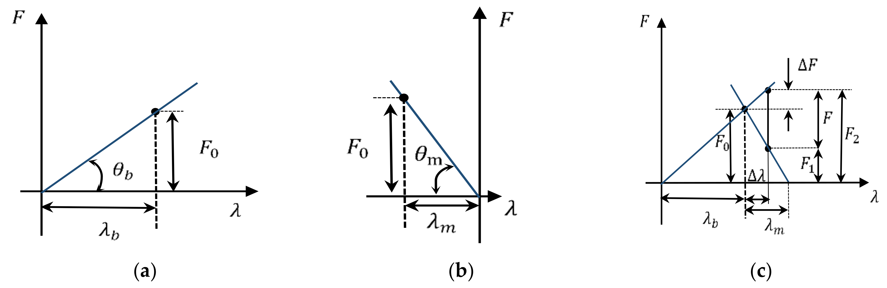
2.1. Maximum Load of the Bolt

The bolt preload is produced by tightening torque during the tightening process, with the direction along the bolt axis. Proper preload contributes to the reliability of the entire system. In this paper, the maximum preload of the bolts was 710 kN and the minimum preload was 548 kN.

The main failure mode of the high-strength bolt is tensile fracture, therefore, in the theoretical calculation only the axial load component was considered. The stress distribution of the bolt at the main shaft-to-hub bolted connection is shown in Figure 1. The bolts are distributed in circumference, and the angle between the two adjacent bolts is $\beta$.

The relationship between the axial load of bolt $F_n$ and the overturning moment $M$ can be stated as:

$$M={\displaystyle \sum _{n=1}^Z{F}_{n}R\cos {\beta }_n},$$

(1)

from which

$${\beta }_n=n\beta ,F_n=F_m\cos {\beta }_n,$$

(2)

where $Z$ is the number of bolts, $F_n$ is the axial load of the bolt produced by overturning moment $M$, and $F_m$ is the maximum axial load produced by the overturning moment. The maximum load of the bolt is found to be:

$$F_{\max }=F_m-\frac{F_z}{Z}=\frac{2M}{ZR}-\frac{F_z}{Z},$$

(3)

where $F_z$ is the axial load of the bolt produced by external axial load of the model. $R$ is the radius of the circumference of the bolt distribution.

2.2. The Working Stress of Bolts

First, the bolt stiffness and the connector stiffness are derived in order to obtain the working stress of the bolt. As shown in Figure 2a,b, the bolt stiffness and the connector stiffness can be expressed as follows:

$$C_b=\tan {\theta }_b=\frac{F_0}{{\lambda }_b},C_m=\tan {\theta }_m=\frac{F_0}{{\lambda }_m}$$

(4)

As seen in Figure 2c:

$$F_2=F_0+\Delta F,$$

(5)

$$\frac{\Delta F}{F-\Delta F}=\frac{\Delta \lambda \tan {\theta }_b}{\Delta \lambda \tan {\theta }_m}=\frac{C_b}{C_m}.$$

(6)

So, the working stress of bolts can be stated as:

$$F_2=F_0+\frac{C_b}{C_m+C_b}F,$$

(7)

where $F_2$ is the working stress of the bolt, $F_0$ is the preload of the bolt, $F$ is the maximum load of the bolt which is equal to $F_{\max }$, and $F_1$ is the remainder preload.

2.3. Stress Cross-Sectional Area of Bolts

According to Chinese National Standards [13], the stress cross-sectional area of the bolt can be stated as:

$$A_s=\frac{\pi }{4}{(\frac{d_2+d_1-\frac{H}{6}}{2})}^2,$$

(8)

where $H$ is the nominal height of the thread, $d_2$ is the middle diameter of the thread, and $d_1$ is the minor diameter of the thread. The stress on the bolt can be found to be:

$$\sigma =\frac{F_2}{A_S}.$$

(9)

3. Finite Element Method Analysis

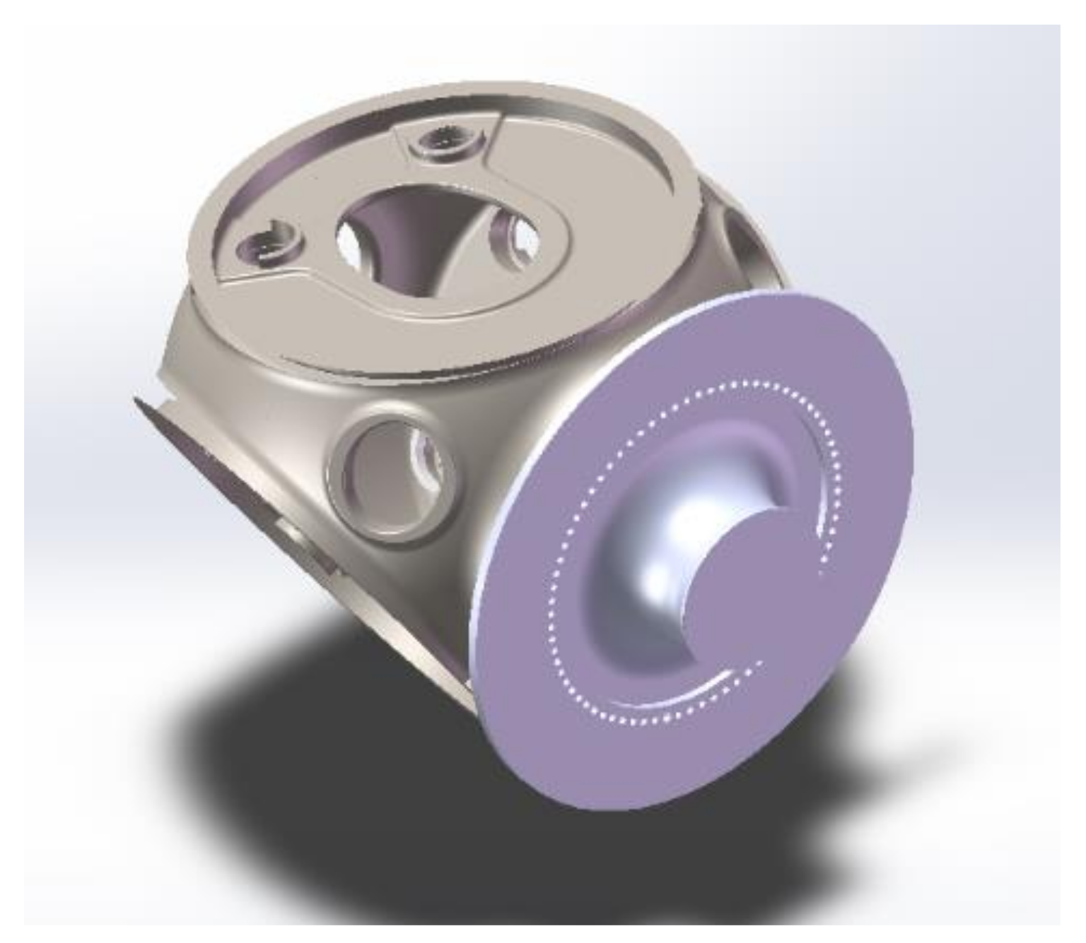
3.1. Geometric Model

The geometrical model was built using SolidWorks software, and is shown in Figure 3. Bolt parameters are shown in

Table 2. Bold parameters.

Item	Parameters
Type size	M39
The class of bolts	10.9
The number of bolts	76
Yield strength	940 MPa
Ultimate strength	1040 MPa
Elastic modulus	$2.1\times {10}^5$ MPa
Poisson’s ratio	0.3
Thread torque	3300 Nm

.

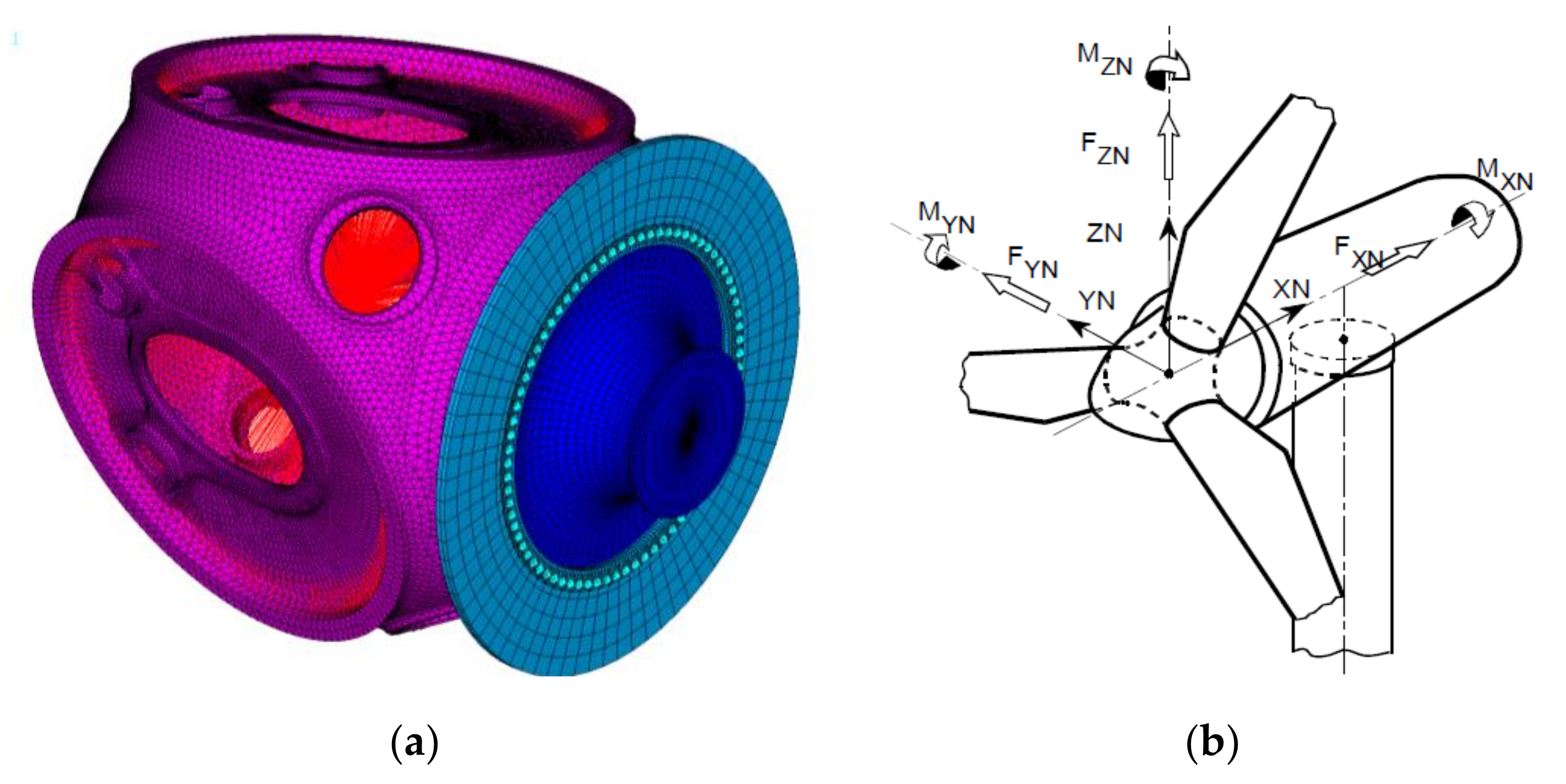
3.2. Finite Element Model

The finite element model is shown in Figure 4a, and the coordinate system of the model is the hub coordinate system according to the GL recommendations [3], as shown in Figure 4b. The hub coordinate system has its origin at the hub center, and does not move with the wind turbine. X-axial is along the shaft axis, z-axial travels upwards perpendicular to x-axial, and y-axial is positioned horizontally.

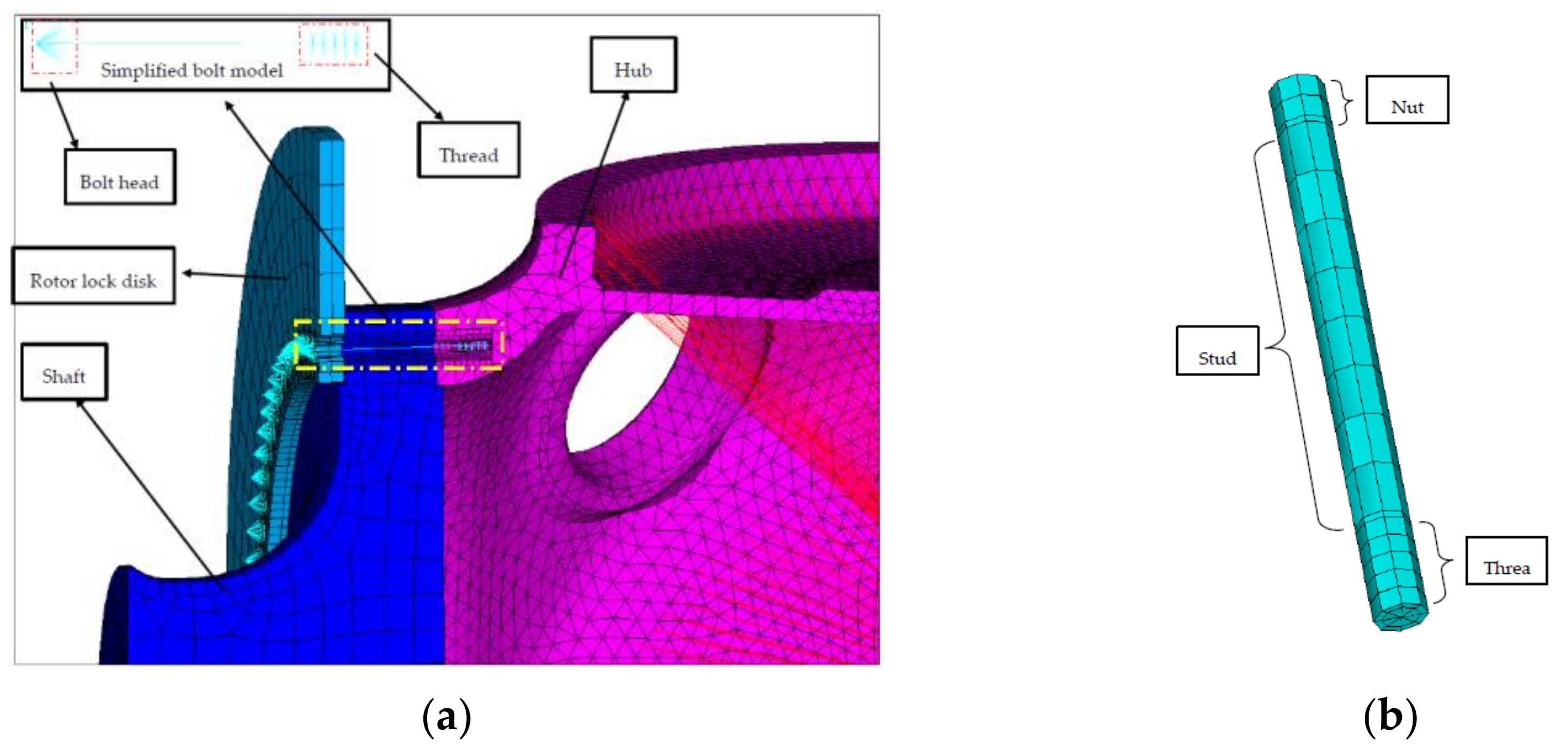
3.2.1. Simplified Bolt Model

The cross section of the finite element model is shown in Figure 5a. The bolt was modeled by Beam188 element using ANSYS software (https://www.ansys.com/) with six or seven degrees of freedom per node as shown in Figure 5a. Fatigue testing of high-strength bolts shows that the position where the bolt can easily cause failure is always near the edge of the thread or the nut [14]. Therefore, a refined element was built in the transition section of the nut and the thread as shown in Figure 5b. The thread was connected with the hub by the beam element as well as the connection between the nut and rotor locking disk. The beam element representing the stud was modeled with real constant properties defined by the nominal diameter of the bolt. Preload was preserved as a displacement in the bolt.

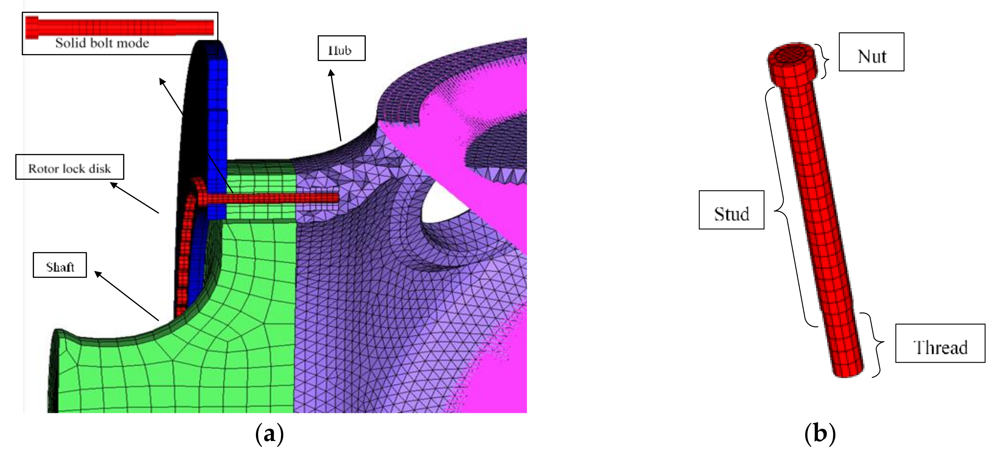
3.2.2. Solid Bolt Model

As shown in Figure 6a,b, the solid bolt model was modeled by the SOLID185 element in ANSYS with eight nodes, and each node contained three degrees of freedom. The boundary condition was the same as the simplified bolt model. The thread connected with the hub by sharing the same nodes as well as the connection between the nut and rotor locking disk. Preload was preserved as a displacement in the bolt.

A detailed description of both finite element models is shown in

Table 3. Summary of finite element models.

Item	Simplified Bolt Model	Solid Bolt Model
Type of bolt element	Beam188	Solid185
Number of bolt nodes	6688	358,644
Number of bolt elements	6612	79,344
Contact behavior	Frictional contact	Frictional contact

.

3.3. Boundary Conditions and Loads

As shown in Figure 7, the boundary condition of the finite element model was that the nodes on the end of the shaft were fixed in all degrees of freedom. The position where loads were applied was the origin of the hub coordinate system connected with the hub by rigid beams. According to the Mechanical Design Handbook [15], the contact friction coefficient between the hub and shaft was 0.22, as well as between the shaft and rotor lock disk.

According to the structural characteristics of wind turbines, the bolts of the main shaft-to-hub bolted connection in a wind turbine are mainly affected by the moment. Consequently, only the following load cases were taken into account. These were calculated using the dynamics software Bladed according to GL recommendations [3], and are shown in

Table 4. Extreme loads at the hub center.

Load Components	${\mathit{M}}_{\mathit{x}}$	${\mathit{M}}_{\mathit{y}}$	${\mathit{M}}_{\mathit{z}}$	${\mathit{F}}_{\mathit{x}}$	${\mathit{F}}_{\mathit{y}}$	${\mathit{F}}_{\mathit{z}}$
Unit	(kNm)	(kNm)	(kNm)	(kN)	(kN)	(kN)
Load case 1	3536.4	1178.7	−927.7	336.4	−809.7	525.3
Load case 2	−2546	1134.1	2657.8	−149.1	708.2	497.9
Load case 3	845.4	9326.6	307.9	128.8	−633.7	−517.9
Load case 4	2994.1	−6103.7	−258	281.1	84.8	922
Load case 5	2762	1069.7	6564.2	215.5	907.6	−353.2
Load case 6	2254.3	−99.7	−6640.5	546.2	923.9	440.6
Load case 7	871.9	9325.3	431.5	131.1	−604	−556.3

. Load case 1 represents that the loads component of $M_x$ is the maximum among the extreme loads, while load case 2 represents that $M_x$ is the minimum, load case 3 represents that $M_y$ is the maximum, load case 4 represents that $M_y$ is the minimum, load case 5 represents that $M_z$ is the maximum, load case 6 represents that $M_z$ is the minimum, and load case 7 represents that $M_{\mathrm{y}z}$ is the maximum. The preload applied in the bolts was 550 kN.

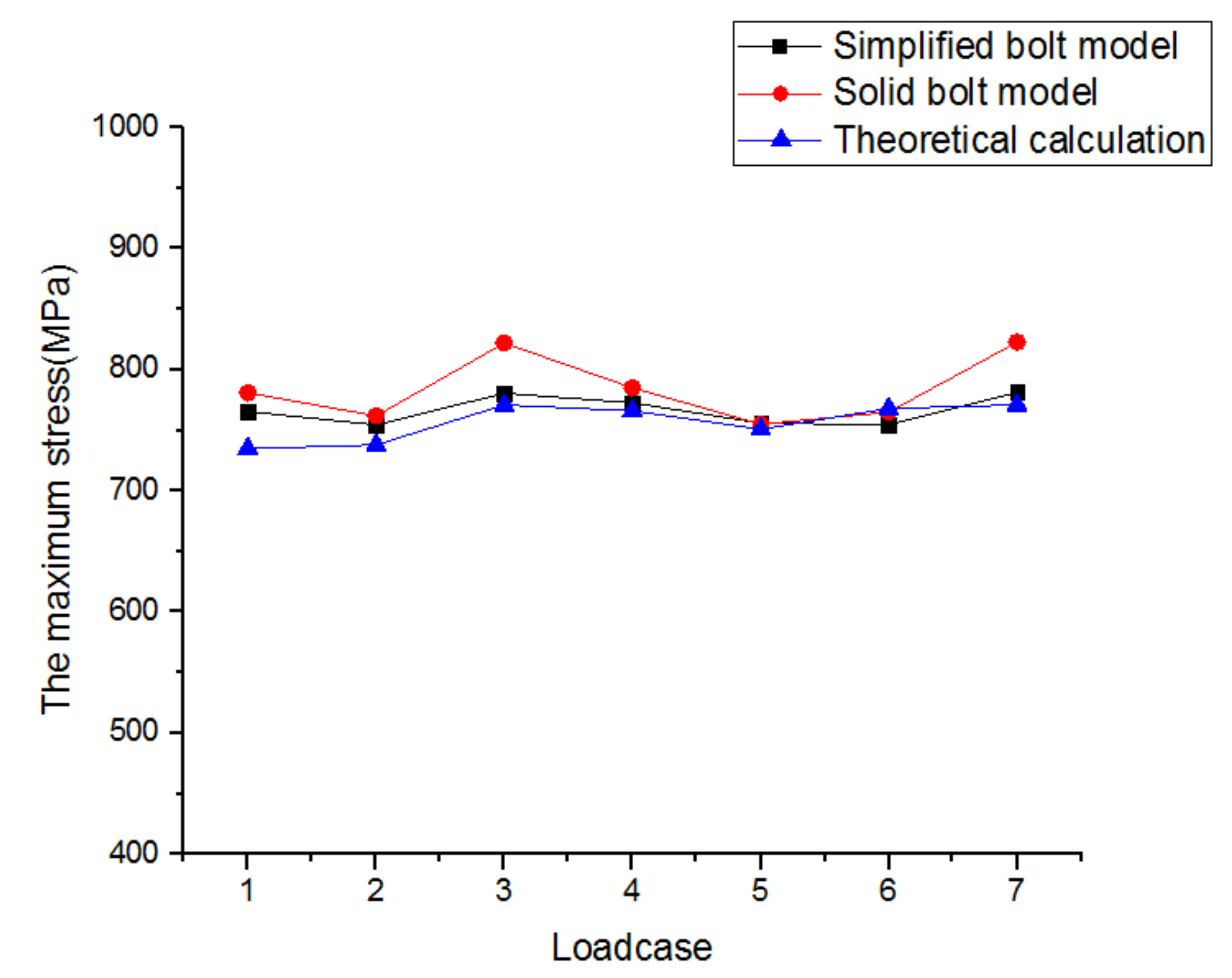
3.4. Finite Element Method Results

The simplified bolt is modeled by the Beam188 element [16] in ANSYS software, which is based on Timoshenko beam theory in consideration of shear-deformation effects. The software can output the stress component results of the Beam188 element directly, which is produced by axial loads and bending, as indicated in the following definitions:

$${\sigma }_{\mathrm{axial}}=\frac{F_x}{A}, {\sigma }_{\mathrm{bending}}=\frac{My}{I},$$

(10)

where ${\sigma }_{\mathrm{axial}}$ is the stress component produced by axial load, $F_x$ is the axial load, $A$ is the area of the element cross section, ${\sigma }_{\mathrm{bending}}$ is the bending-stress component, $M$ is the bending moment of the beam, $y$ is the distance from the neutral axis, and $I$ is the moment of inertia of the cross section.

As in the finite element model, the bolt element was modeled with real constant properties defined by the nominal diameter of the bolt, which is greater than the thread diameter, so the stress output should be factored to compensate for the difference in cross-sectional area between the stud cross section and the thread cross section.

The axial stress component and the bending stress component of the bolt should be compensated with the following factors:

$$K_A=\frac{A_N}{A_S}, K_B={(\frac{D_N}{D_S})}^3,$$

(11)

where $A_N$ is the stud cross section area, $A_S$ is the thread cross section area, $D_N$ is the nominal diameter, and $D_S$ is the thread diameter.

The resultant bolt stress is calculated as follows:

$${\sigma }_{\mathrm{res}}=K_A{\sigma }_{\mathrm{axial}}+\sqrt{{(K_B{\sigma }_{\mathrm{bending},1})}^2+{(K_B{\sigma }_{\mathrm{bending},2})}^2}.$$

(12)

According to VDI 2230 [17], the working stress of bolts is calculated as follows:

$${\sigma }_{\mathrm{res},\mathrm{total}}=\sqrt{{\sigma }_{\mathrm{res}}{}^2+3(\frac{M_G}{W_P}{)}^2},$$

(13)

where $M_G$ is the value of the tightening torque during the thread (thread torque) and is the polar moment of resistance of the bolt cross section.

The solid bolt model is modeled by SOLID185 element in ANSYS, therefore the von Mises equivalent stress results of bolts can be output directly by the software.

4. Result Analysis

Finite element models were calculated by a PC powered by a 2.53-GHz Quad processor with 48 GBs of random-access memory. Results from the three methods are shown in Figure 8. The result of the simplified bolt model and the solid bolt model were almost consistent. The theoretical derivation was lower as a consequence of ignoring the interaction between bolts and instead only considering the axial load component. Moreover, the simplified bolt model saved nearly 60% of the computational time and 19% of the memory usage in comparison with the solid bolt model shown in

Table 5. Results of finite element model (FEM) analysis.

Item	Simplified Bolt Model	Solid Bolt Model	Reduction
Computational time (min)	39.12	15.85	59.48%
Memory usage for resultant file (MB)	1236.31	1003.89	18.80%

. Hence, in terms of efficiency and accuracy, the simplified bolt model is the best choice, with guaranteed accuracy.

5. Fatigue Analysis of Bolts

According to the above study, the simplified model was used in the fatigue life analysis of bolts. Above all, the stress spectrum for bolts was computed based on the simplified model. The fatigue failure mode of wind turbines is high-cycle fatigue on account of the fatigue loads of wind turbines in operation. The stress history of the wind turbine was then analyzed by means of rainflow counting, and the results were corrected using the Goodman relation. Finally, the fatigue life of bolts was obtained based on S–N curve and linear damage accumulation assumption. The main method and principle used are introduced as follows.

5.1. Stress Spectrum for Bolts

Based on the simplified bolt model method, the relationship between the six load components and bolt stress can be obtained by the fitting of a polynomial as shown in Figure 9a,b, so that the fatigue loads spectrum can be transformed into the stress spectrum of the bolt by linear superposition as described in Figure 10. Fatigue loads of the simplified model within twenty years for the six load components at the hub center were computed using Bladed software, and part of the fatigue loads spectrum within three hours is shown in Figure 10. The stress spectrum for the bolt can then be used for fatigue calculations.

5.2. Rainflow Counting

Rainflow counting is used to summarize a variable amplitude stress or strain history and to obtain the number of cycles with different amplitude and mean values. This is a widely-used approach in fatigue calculations [18,19,20]. It is assumed that each cycle can contribute to a certain degree of fatigue damage to the material, ignoring the influence of the material memory connected with plastic strains generated while successive loading cycles in the determination of fatigue life.

Rainfall counting is like raindrops flowing down the top of a multi-story tower from top to bottom, thus the name “rainflow counting”. The principle of rainflow counting is to rotate the coordinate system of the stress spectrum by 90 degrees so that the time coordinate axis is facing downwards. It is assumed that the rain begins to flow down at the maximum peak (or minimum valley) until it encounters a larger peak or smaller valley below, thus making it a cycle. When a rainflow encounters additional rainflow falling from the upper stream, it stops flowing and becomes a cycle. All cycles are then counted, and the amplitudes and mean values of each cycle are listed.

In this paper, rainflow counting is used to summarize the stress spectrum of bolts in order to obtain the number of cycles $n_i$ with different stress amplitudes and mean stress. The basic method for this paper was produced in a MATLAB environment.

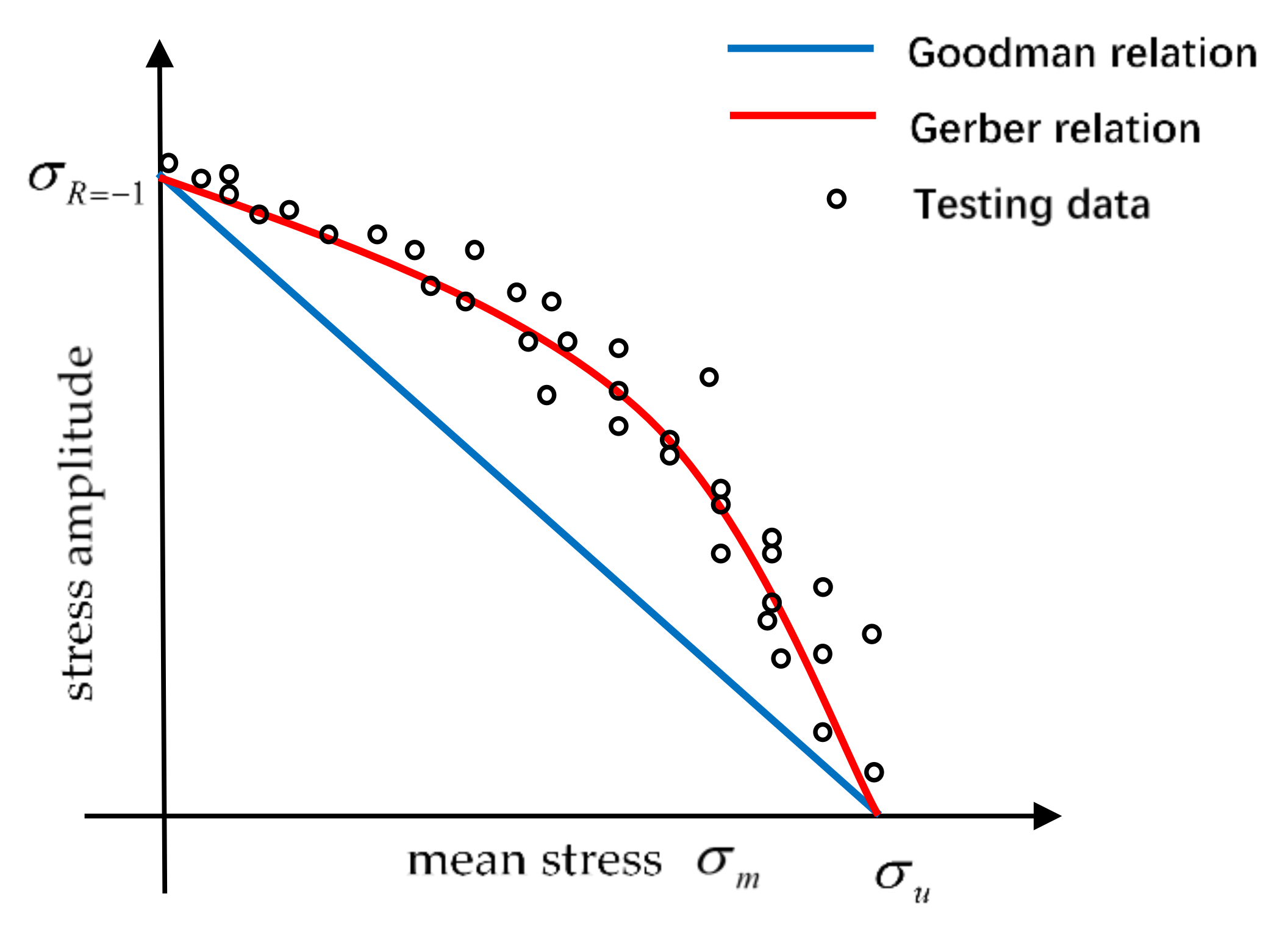
5.3. Mean Stress Correction

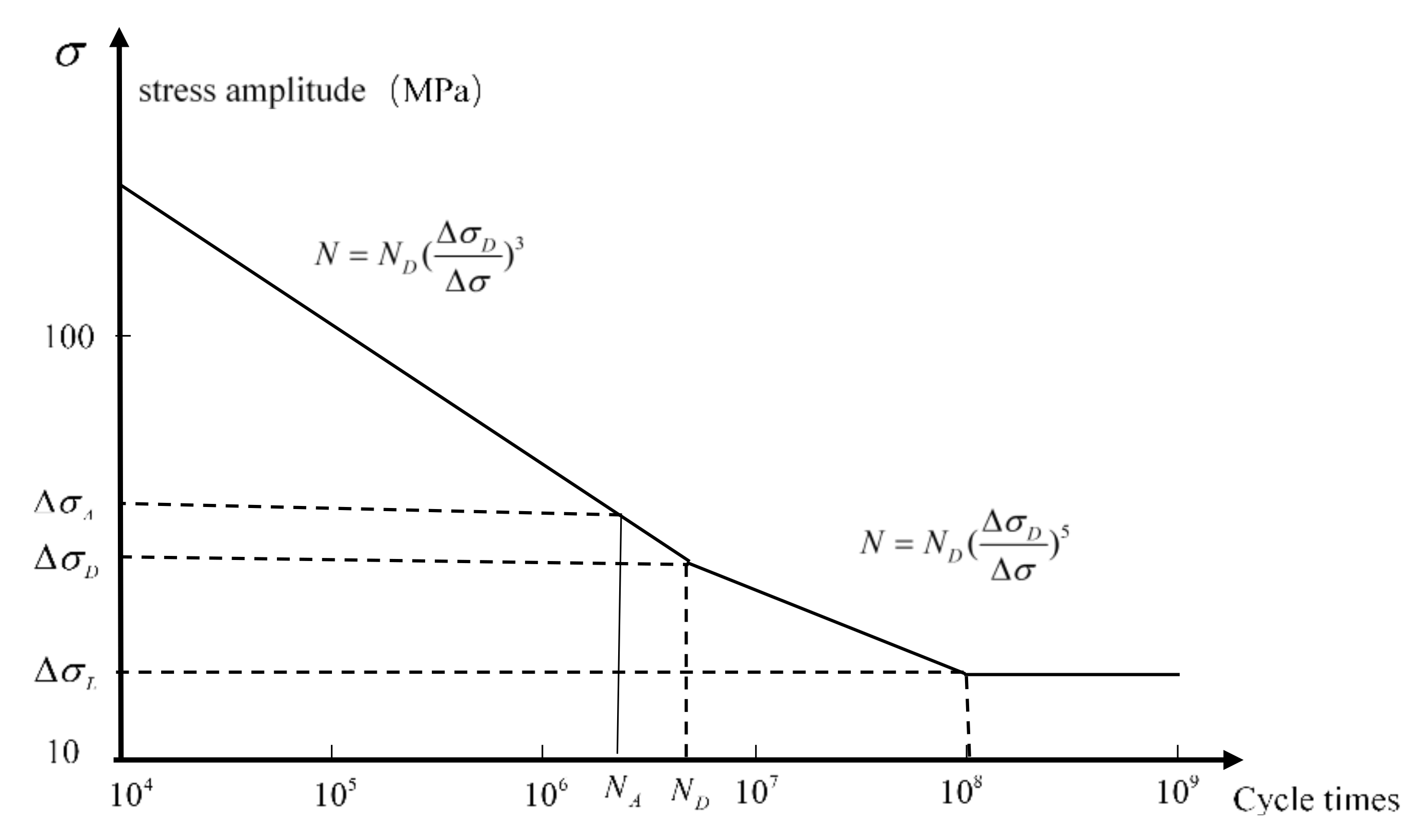
The stress amplitude of the random load spectrum in each cycle is the dominating factor that has an influence on fatigue life, but fatigue life is also affected by mean stress. Consequently, the effect of mean stress needs to be taken into consideration in fatigue analysis.

It has been proven that mean stress decreases with the increasing stress amplitude at the same level of fatigue life by a large number of tests. The Gerber relation [21] describes the relationship between mean stress and stress amplitude through a curve model, which is consistent with the test results. The Goodman relation [22] represents the relationship between the mean stress and the stress amplitude by a straight line. Most experimental results were above this line, so the Goodman relation was more conservative, as shown in Figure 11. The effect of mean stress was determined by the Goodman relation in this paper, which can be expressed as the following form:

$${\sigma }_a=(1-\frac{{\sigma }_m}{{\sigma }_u}){\sigma }_{R=-1},$$

(14)

where ${\sigma }_u$ is the ultimate strength of the material, ${\sigma }_a$ is stress amplitude, ${\sigma }_m$ is mean stress, and ${\sigma }_{R=-1}$ is the cut-off limit when the stress ratio $R=-1$.

Because the S–N curve of a material is obtained when the stress ratio $R=-1$, stress amplitudes and mean stress obtained by rainflow counting were corrected by Goodman relation.

5.4. S–N Curve

The S–N curve displays the relationship between the elastic stress of materials and the number of cycles when fatigue damage occurs, where S represents the stress amplitude and N is the number of fatigue cycles. To some degree, the stress amplitude and the fatigue life are in inverse proportion to each other. The S–N curve is plotted by a large number of fatigue tests [23], considering the influence of the surface roughness factor, safety factor, stress ratio, geometric characteristics (e.g., notch, weld, etc.), and surface treatment coefficient.

According to the fatigue damage features, fatigue damage can fall into two categories: low-cycle fatigue and high-cycle fatigue. The fatigue in wind turbine components is high-cycle fatigue. The numerical models suitable for high-cycle fatigue mainly consist of the Basqui model [24], the Langer model [25], and the three-parameter model [26]. The Basqui model, which is widely used in high-cycle fatigue, is defined as:

$$S^{m}N=C,$$

(15)

where m and C are parameters related to the surface roughness factor, safety factor, stress ratio, geometric characteristics, and so on.

The cycle times $N_i$ under different stress amplitudes can be obtained when the bolt experiences fatigue failure through the S–N curve. The Basqui model is used to produce the S–N curve in this paper. According to the GL recommendations [3] and Eurocode 3 [27], for the S–N curve of high-strength bolts, when the number of stress cycles $N<5\times {10}^6$, the slope of the curve is 3; when the number of stress cycles $N>5\times {10}^6$, the slope of the curve is 5. According to the GL recommendations, for bolts rolled after heat treatment and larger than M30, the detail category of stress amplitude is calculated as follows when the number of cycles is $2\times {10}^6$:

$$\Delta {\sigma }_{\mathrm{A},\mathrm{red}}=0.85·{(\frac{30}{d})}^{0.25}·(\frac{150}{d}+45).$$

(16)

The S–N curve of the bolt is shown in Figure 12.

5.5. Linear Damage Cumulative Rules

Under the linear damage cumulative rules, all stress is independent and isolated in the cycle loading. The fatigue of materials is proportional to the work absorbed by the materials. The stress amplitude and average stress contribute to the same degree of failure which is linearly accumulated, ignoring the effect of the loading sequence in fatigue life evaluation. The failure of materials is assumed to occur when the cumulative damage reaches a certain level

The Palmgren–Miner linear damage accumulation hypothesis [28], which is the most widely used model, is validated by fatigue tests [29,30]. It can be expressed as:

$$D={\displaystyle \sum _{i=1}^k\frac{n_i}{N_i}}\le D_{\max }=1,$$

(17)

where $k$ is the number of different stress amplitudes, $D_{\max }$ is the accumulated damage sum when the failure of materials occurs, and $D$ is the accumulated damage within 20 years. Based on the above theory, the maximum damage to bolts was $1.2\times {10}^{-5}\le 1$ as obtained by programming the algorithm in MATLAB software (https://www.mathworks.com/), which meets the wind turbine design requirements according to GL recommendations [3].

6. Conclusions

In this paper, the strength of the main shaft-to-hub bolted connection in a wind turbine was analyzed by theoretical derivation and two different kinds of modeling methods. The fatigue life of bolts was analyzed under multiple random loads based on the simplified bolt model and fatigue theory. The conclusions are summarized as follows.

From the results of static analysis, the bolt strength analysis results of the simplified model were similar to those of the solid model, while the stress on bolts obtained by theoretical derivation were lower. However, the simplified bolt model saved nearly 60% of the computational time and 19% of the memory usage in comparison with the solid bolt model. Therefore, in terms of efficiency and validity, the simplified bolt model is a better choice in ultimate strength and fatigue life analysis of wind turbine bolts.

References

1. Burton, T.; Sharpe, D.; Jenkins, N.; Bossanyi, E. Wind Energy Handbook; John Wiley & Sons, Ltd.: New York, NY, USA, 2001; pp. 421–423. [Google Scholar]
2. Chu, W.Y.; Li, S.Q.; Hsiao, C.M.; Yao, Y.Q. Fracture analysis of high strength bolt. Phys. Exam. Test. 2010, 16, 149. [Google Scholar]
3. Lloyd, G. Strength Analyses. In Guideline for the Certification of Wind Turbine; Germanischer Lloyd Industrial Services GmbH: Hamburg, Germany, 2010; pp. 5–14. [Google Scholar]
4. Schmidt, H.; Neuper, M. Zum elastostatischen Tragverhalten exzentrisch gezogener LStöße mit vorgespannten Schrauben. Stahlbau 1997, 66, 163–168. [Google Scholar]
5. Petersen, C. Stahlbau—Grundlagen der Berechnung und Baulichen Ausbildung von Stahlbauten (Steel Construction—Basics of the Dimensioning and the Constructional Formation of Steel Constructions), 3rd ed.; Vieweg: Braunschweig, Germany, 1993. [Google Scholar]
6. Seidel, M. Ermittlung der ermüdungsbeanspruchung von schrauben exzentrisch belasteter flanschverbindungen. Stalhbau 2001, 70, 474–486. [Google Scholar] [CrossRef]
7. Huang, Y.H.; Wang, R.H.; Zou, J.H.; Gan, Q. Finite element analysis and experimental study on high strength bolted friction grip connections in steel bridges. Steel Constr. 2010, 66, 803–815. [Google Scholar] [CrossRef]
8. Kim, J.; Yoon, J.C.; Kang, B.S. Finite element analysis and modeling of structure with bolted joints. Appl. Math. Model. 2007, 31, 895–911. [Google Scholar] [CrossRef]
9. Yorgun, C.; Dalcı, S.; Altay, G.A. Finite element modeling of bolted steel connections designed by double channel. Comput. Struct. 2004, 82, 2563–2571. [Google Scholar] [CrossRef]
10. Braccesi, C.; Cianetti, F.; Lori, G.; Pioli, D. Random multiaxial fatigue: A comparative analysis among selected frequency and time domain fatigue evaluation methods. Int. J. Fatigue 2015, 74, 107–118. [Google Scholar] [CrossRef]
11. Matjaž, M.; Slavič, J.; Boltežar, M. Frequency-domain methods for a vibration-fatigue-life-estimation—Application to real data. Int. J. Fatigue 2013, 47, 8–17. [Google Scholar]
12. Braccesi, C.; Cianetti, F.; Lori, G.; Pioli, D. Evaluation of mechanical component fatigue behavior under random loads: Indirect frequency domain method. Int. J. Fatigue 2014, 61, 141–150. [Google Scholar] [CrossRef]
13. Chinese National Standards. GB/T 16823.1-1997. Stress Area and Bearing Area for Threaded Fasteners; Chinese National Standards: Beijing, China, 1997. [Google Scholar]
14. Tian, J.; Shang, G.G.; Zhou, J.B.; Zhu, Y.M. Fatigue Life Analysis of the High Strength Connecting Rod Bolt. J. Nanjing For. Univ. 2005, 5. [Google Scholar] [CrossRef]
15. Editorial Board of Mechanical Design Manual. Mechanical Design Handbook (New Version); China Machine Press: Beijing, China, 2004; Volume 1, pp. 1–23. ISBN 9787111147332. [Google Scholar]
16. Swanson Analysis Systems Inc. ANSYS User’s Manual, Version 15.0; Swanson Analysis Systems Inc.: Houston, PA, USA, 2013. [Google Scholar]
17. Verein Deutscher Ingenieure. VDI 2230 Part 1. Systematic Calculation of High Duty Bolted Joints, Joints with One Cylindrical Bolt; Verein Deutscher Ingenieure: Düsseldorf, Germany, 2003. [Google Scholar]
18. ASTM International. 1985 ASTM E 1049-85. Standard practices for cycle counting in fatigue analysis. In Annual Book of ASTM Standards; ASTM International: Philadelphia, PA, USA, 1999; pp. 710–718. [Google Scholar]
19. Socie, D.; Marquis, G.B. Multiaxial Fatigue; Society of Automotive Engineers, Inc.: Warrendale, PA, USA, 1999; pp. 246–250. [Google Scholar]
20. Niesłony, A. Determination of fragments of multiaxial service loading strongly influencing the fatigue of machine components. Mech. Syst. Signal Process. 2009, 23, 2712–2721. [Google Scholar] [CrossRef]
21. Gerber, W.Z. Calculation of allowable stresses in iron structures. Z. Bayer Arch. Ing. 1874, 6, 101–110. [Google Scholar]
22. Hertzberg, R.W.; Hauser, F.E. Deformation and fracture mechanics of engineering materials. Wiley 1976, 19, 283. [Google Scholar] [CrossRef]
23. British Standard Institute (BSI). BS7608-1993 Fatigue Design and Assessment of Steel Structures; BSI: London, UK, 1993. [Google Scholar]
24. Basquin, O.H. The Exponential Law of Endurance Tests. Am. Soc. Test. Mater. Proc. 1910, 10, 625–630. [Google Scholar]
25. Langer, B.F. Design of pressure vessels for low cycle fatigue. J. Basic Eng. ASME 1962, 84, 389–602. [Google Scholar] [CrossRef]
26. Weilbull, W. Fatigue Testing and Analysis of Results; Pergamon Press: London, UK, 1961; pp. 107–112. [Google Scholar]
27. ECCS-European Convention. Fatigue Design of Steel and Composite Structures. In Eurocode 3: Design of Steel Structures. Part 1–9; ECCS, Ernst & Sohn: Berlin, Germany, 2011; pp. 18–33. [Google Scholar]
28. Miner, M.A. Cumulative damage in fatigue. J. Appl. Mech. 1945, 12, 159–164. [Google Scholar]
29. Fatemi, A.; Yang, L. Cumulative fatigue damage and life prediction theories: A survey of the state of the art for homogeneous materials. Int. J. Fatigue 1998, 20, 9–34. [Google Scholar] [CrossRef]
30. Jeelani, S.; Musial, M. A study of cumulative fatigue damage in AISI 4130 steel. J. Mater. Sci. 1986, 21, 2109–2113. [Google Scholar] [CrossRef]
Figure 1. The stress distribution of the main shaft-to-hub bolted connection.
Energies 12 00007 g001
Figure 2. (a) The schematic of bolt stiffness; (b) The schematic of connector stiffness; (c) The relationship between bolt stiffness and connector stiffness.
Energies 12 00007 g002
Figure 3. Geometry used for finite element analysis (FEA).
Energies 12 00007 g003
Figure 4. (a) FEA model of main shaft-to-hub bolted connection; (b) Hub coordinate system.
Energies 12 00007 g004
Figure 5. (a) Cross section of the finite element model; (b) Simplified bolt model.
Energies 12 00007 g005
Figure 6. (a) Cross section of the finite element model; (b) Solid bolt model.
Energies 12 00007 g006
Figure 7. Boundary conditions.
Energies 12 00007 g007
Figure 8. The maximum stress of bolts under extreme load.
Energies 12 00007 g008
Figure 9. (a) The relationship between the force components and bolt stress; (b) The relationship between the moment components and bolt stress.
Energies 12 00007 g009
Figure 10. Part of stress spectrum for bolt.
Energies 12 00007 g010
Figure 11. Mean stress effect correction.
Energies 12 00007 g011
Figure 12. S–N curve for a high-strength bolt.
Energies 12 00007 g012