1. Introduction
Since the end of the 20th century, autonomous robots have been used in tasks where the presence of divers is costly, dangerous, or even impossible. There is an important interest in these robots for the maintenance of marine renewable energy (MRE) systems (underwater devices such as offshore wind turbines, tidal turbines, or hydroelectric dam underwater structures). Moreover, there are also interests in military applications (mine warfare, sensitive areas protection) and for offshore industry activity (pipelines or telecommunication cables).
For these missions, underwater interventions on complex structures (hostile environment) require autonomous underwater vehicles (AUVs) with enhanced maneuvering capabilities [
1]. These more stringent demands imply the need to expand the capabilities of AUVs such as speed, power, control, and perception. However, the propulsion and control systems for this robot kind have not improved as quickly as their needs, which restricts their performance and thus their autonomy. According to [
2], it is necessary to give long range and maneuvering capabilities to AUVs to advance to a new generation of underwater robots able to perform a more extensive set of operations. What refers to two design aspects of these vehicles: hull shape and propulsion system. [
1] observes that investigations and developments have been conducted about underwater vehicles locomotion, but few are dedicated to the propulsion system. Therefore, this is our research focus.
The propulsion systems of underwater vehicles can be divided into three categories [
2]:
Classical rear propeller with control surface architectures, as in large conventional submarine equipped with rudders;
Biomimetic propulsion, i.e., inspired by natural propulsion mechanisms present in marine life, e.g., dolphin and whale fins;
Vectorial thrust (VT), which can be achieved with one or a set of propellers, whose thrust vectors drive and steer the vehicle without the need for control surfaces.
It is immediate that the propulsion architecture of a vehicle determines its set of possible motion directions as well as influences the ability to control the movement. The first category of propulsion systems offers low maneuverability and the second one is difficult to implement or control [
3,
4,
5,
6].
In VT propulsion systems, it is possible to drive and steer the vehicle only using thrusters through various strategies. One possibility is to use a set of fixed thrusters (FT) [
7]. A single FT endows the robot with only a thrust vector which does not allow trajectory tracking. This issue is solved with the combination of several FTs acting in different directions and with different thrust, e.g., water-jet thrusters. Another possibility is to use a few or a single reconfigurable thruster (RT), since they may have their thrust vectors redirected, which involves more than one degree of freedom (DOF) [
8,
9].
One of the RT systems advantages over FT ones is the possibility of reducing the number of thrusters to the minimum, which reduces the total vehicle mass. Another advantage is the reduced consumption of energy when changing directions [
2]. However, to guarantee a greater maneuverability and increased controllability of AUVs, an RT must be endowed with the greatest possible capability to reorient its thrust vector [
10].
Recently, researches have been carried out to advance in the development of different RT types. A research team developed spherical-shaped underwater vehicles with three [
11] and four [
12] reconfigurable water-jet thrusters, with 2-DOF of reconfiguration each, but using waterproof servomotors (IP67 protection). Ref. [
13] developed a small underwater vehicle with an RT based on nozzle orientation that redirects the propeller exhaust flow with 2-DOF, keeping the propeller without contact with marine life, and not requiring any shaft reorientation. Ref. [
14] also developed an RT with 2-DOF of propeller and duct reconfiguration using a spherical parallel mechanism. In [
15], authors analyzed the state-of-the-art in key technologies for AUVs and indicate that the VT technologies are not yet mature and due it, they propose an orientable motor-to-propeller transmission mechanism, based on ball gear, with wide range wrist rotation. However, their review did not take into account the advances in RMCTs [
1], since they analyzed only mechanical transmission systems. Excluding [
11], all these projects indicate that:
They do not need to reorient their motor axis to reconfigure the thrust vector. Only their propeller, duct or nozzle must be reoriented. Thus, reduced power and torque values are required in the maneuvers.
They need three actuators to ensure 2-DOF of VT reconfiguration.
They need mechanical seals, since the movement is transmitted through shafts or rods, which implies frictions and likely watertightness issues.
The watertightness issue is more critical in deep-water tasks, due to high pressure. Also due to this, we proposed a new vectorial thruster based on reconfigurable magnetic couplings, which is named reconfigurable magnetic coupling thruster (RMCT) [
10]. In this thruster, the motor shaft movement is transmitted to the propeller one at a distance, without any material medium, through a magneto-mechanical device which works as a coupling and/or joint allowing the propeller driving and orientation. This brings benefits [
16] such as:
Movement transmission between insulated environments
Complex and unsure mechanical seals are no longer needed
Robot watertightness is not jeopardized by a hull breach
It eliminates the friction inherent to mechanical seals and joints
The magnetic coupling also works as a mechanical fuse (torque limiter) to protect the motor in case of severe load peaks (where a gearbox would break)
Eventual vibrations are mitigated (spring effect)
Low maintenance when it is compared to a mechanical coupling or a universal joint
The challenge in this proposal lies in difficulty of implementing two mechanical functions, jointly: the transmission torque function (coupling) at the distance with the hull in between, and the 3D rotational freedom (spherical joint). Seeking it, we have proposed the first RMCT, the spherical one [
1], with magnets just in one side of the coupling (motor), which results in a low transmitted torque. Recently, we have started to develop a new RMCT version, the radial one [
17]. In [
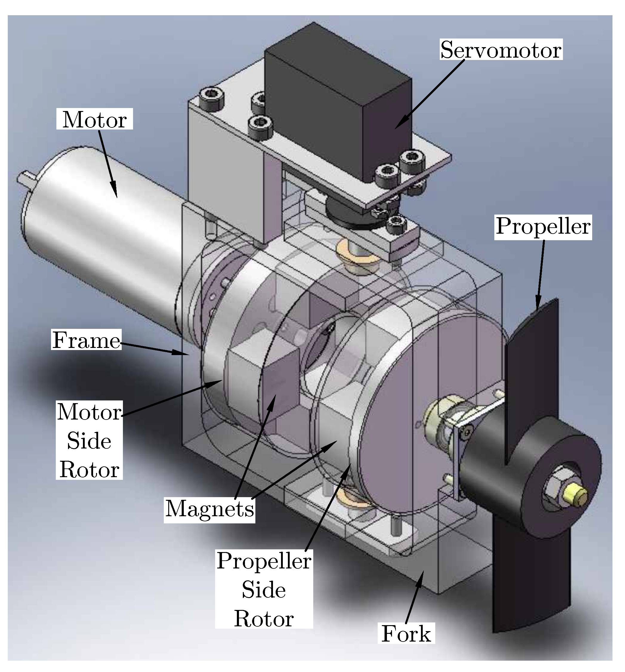
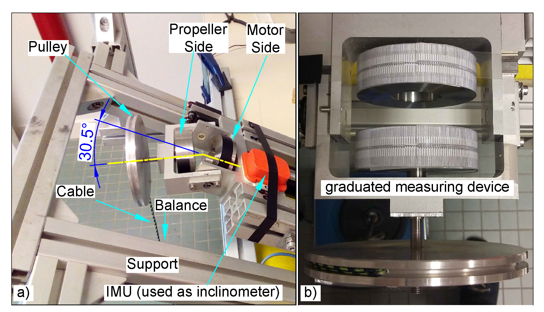
18], we presented the flat reconfigurable magnetic coupling thruster (Flat-RMCT, see
Figure 1), modeling the magnetic torque using partial domain simulation results with a commercial software (Flux3D) achieved by TE2M. TE2M (
www.te2m.fr) is a French company based in Brest specialized on solutions for magnetic systems in high value products industry.
As the Flat-RMCT technology needs a detailed presentation, the present work aims at a further understanding on its coupling torque mechanism. Since this coupling is based on permanent magnets attraction, it has a steady-state synchronous behavior and its causes can be analyzed in detail using a magnetostatic model. In transient-state, besides small oscillations, the coupling can also be considered synchronous. These small oscillations do not generate significant losses, which do not generate a damping effect [
19]. The magnetic torque behavior is fully described using analytical and numerical models validated with real-world experiments on our prototype (
Figure 1). The numerical magnetostatic model adopted is the finite volume integral method [
20] implemented in the RADIA 3D tool [
21] for Mathematica
TM Wolfram language [
22]. It is expected to be able to answer the bellow RMCT questions:
What is the complete reconfigurable magnetic coupling torque behavior, and how does it depend on all angles?
What torque must the servomotor apply to control the propeller orientation?
Once its characteristics are precisely known, it will be possible to simulate, design, and control a Flat-RMCT for AUVs.
This work is organized as follows. In
Section 2 the studied magnetic coupling is discussed. In
Section 3, the magnetostatic numerical model is presented. In
Section 4, the numerical model is validated experimentally, simulated to investigate the RMCT torques behavior, and the results are discussed. The last section gives the conclusion, ongoing works, and perspectives.
2. The Flat Reconfigurable Magnetic Coupling Thruster or Flat-RMCT
The RMCT design has been improving. These improvements have focused on increasing the magnetic coupling torque in intensity and quality. First, we developed the Spherical-RMCT [
1] and then the Flat-RMCT [
18] (
Figure 1) with a better torque transmission. The Flat-RMCT uses two parts of conventional axial permanent magnetic couplings but using flat shaped magnets (parallelepipedic), which makes easier its fabrication.
The conventional axial permanent magnetic couplings are not new [
23,
24], and were also denominated face type couplings [
25]. Often, an axial magnetic coupling has two rotors with magnets assembled on soft-iron yokes, which concentrates the magnetic flux and increases the air gap magnetic energy density [
26]. Usually, others magnetic couplings, besides axial ones, have their driving and driven axes parallels. However, since magnetic gears are also magnetic couplings, there are some couplings with nonparallel axes, e.g., the bevel gear [
27]. Even so, they were always using fixed axes before we have proposed reconfiguring their output axis orientation [
10,
28], disregarding the permanent-magnet spherical actuators [
29], which have other applications not transmitting output shaft torque or speed, but controlling a multidegree-of-freedom joint orientation.
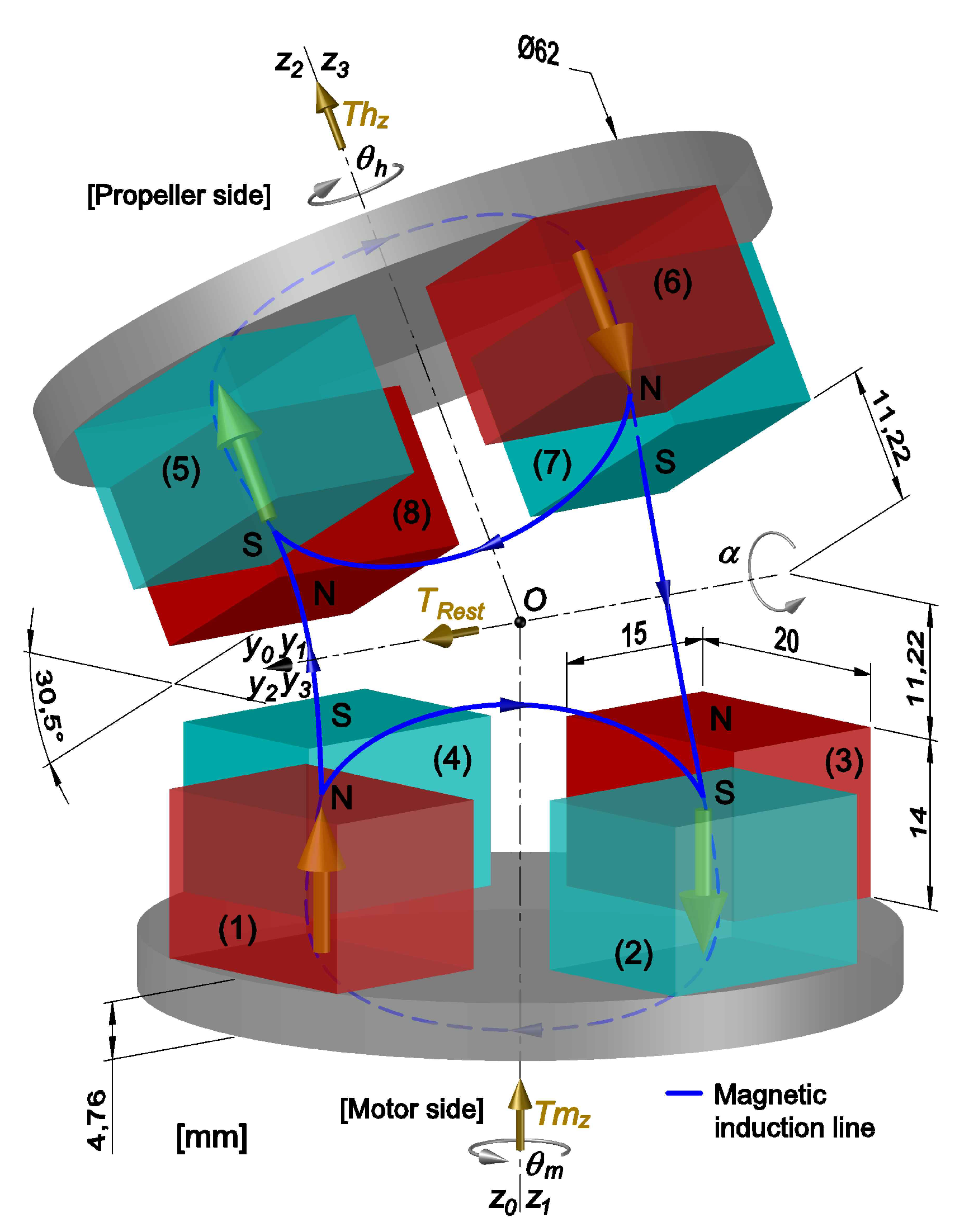
Figure 2 shows the Flat-RMCT. For more details about the mechanical model see [
18]. The figure shows the magnetic parts without their nonmagnetic protection cover against water (jackets). Naturally, the quantity and material type of magnets affect the coupling torque values. We have eight equal samarium cobalt magnets (
) placed 90 degrees between each other, with the remnant magnetization
, made by TE2M company. The magnets colored in blue have their south pole facing the air gap, and the red ones are in the other way. Both soft-iron yokes of rotors are made of steel Z8C17 (magnetic stainless steel), with their diameter equal to 62 mm and thickness equivalent to
mm. The blues lines indicate the two more important magnetic induction lines: the circuit between two magnets in the same part (e.g., magnets (1) and (2)), and a bigger circuit including four magnets, two on each side (e.g., magnets (1), (5), (6) and (2)). There are four frames. The global frame 0 (
) is linked to the robot (frame fixed). Frame 1 (
) is linked to the motor side rotor, rotating
(motor rotor angle) around
. Frame 2 (
) is linked to the fork, rotating
(reconfiguration angle) around
. In addition, frame 3 (
) is linked to the propeller side rotor, rotating
(propeller rotor angle) around
. In any configuration the frames origins are in
O.
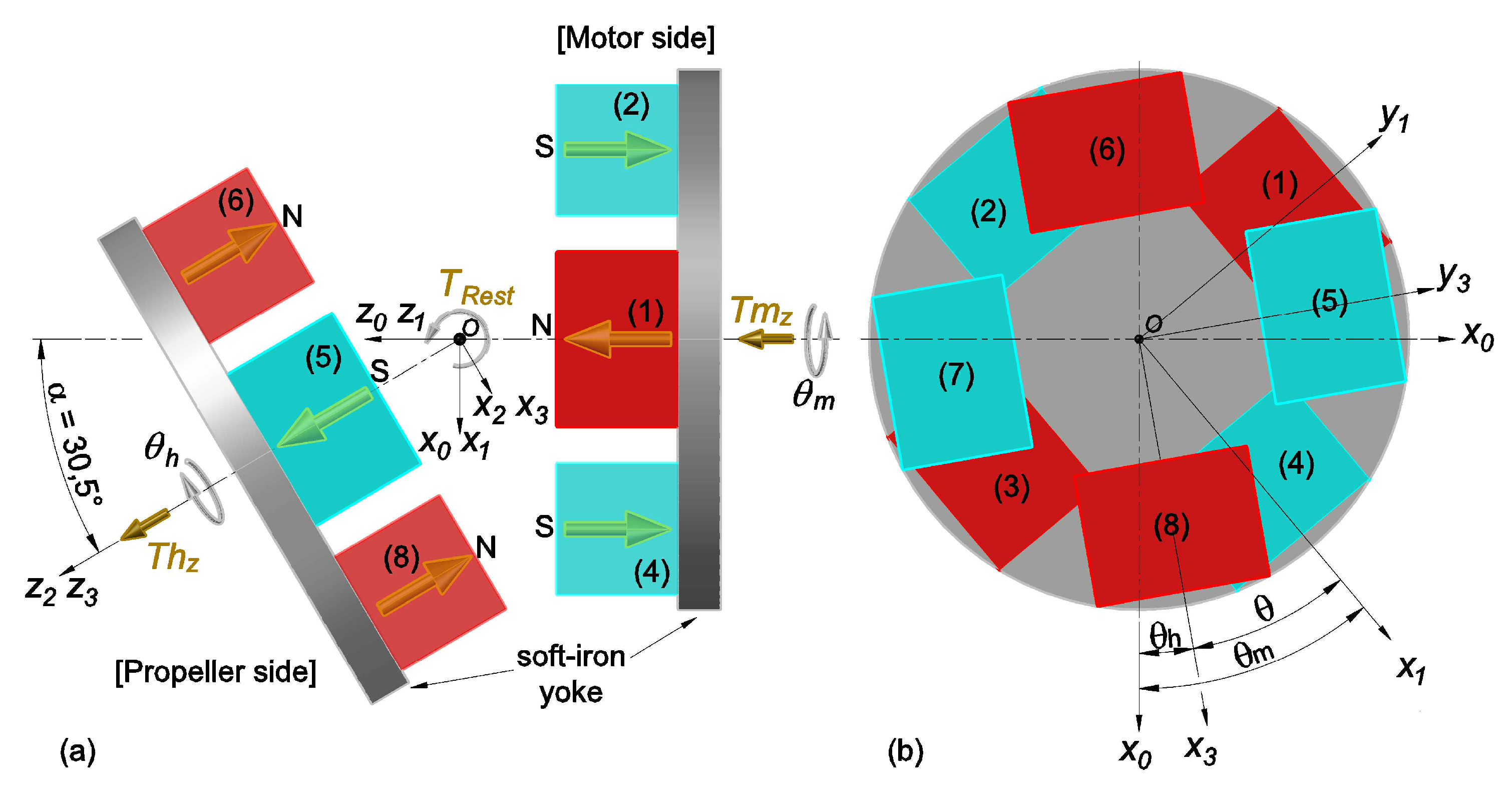
In
Figure 2 and
Figure 3a, the coupling is showed with its maximum reconfiguration angle,
°, when magnets (4) and (8) are closest and magnets (2) and (6) are farthest, and with
°, i.e., when the magnets on motor side are aligned with those on propeller side: stable state with the
minimum magnetic reluctance (MMR). The distance between the reconfiguration axis
and the plane that contains the magnets faces is equal to
mm, which defines a variable air gap with height equal to
mm when
°. It is important to point out that the torque transmission capacity is highly sensible to any air gap change.
In practice, the magnetic reluctance principle implies that the system always seeks the more aligned configuration (north pole with south pole) with lowest air gaps (if possible, with contact between north and south pole), reducing the reluctance and thus increasing the magnetic flux. This principle makes the coupling to work as a rotational nonlinear spring driven by the
magnetic spring angle , generating the
magnetic spring torque :
We should have a stable configuration when
° (with the magnets alignments (1)–(5), (2)–(6), (3)–(7) and (4)–(8)) and also for
° (with the magnets alignments (1)–(7), (2)–(8), (3)–(5) and (4)–(6)), due the coupling symmetry. These stable positions (
) with no spring effect should present a magnetic spring torque
[
18]. There are other configurations where
should be null but completely unstable. It occurs when the equals poles are aligned (closest), i.e., when
. It is expected
in all other configurations when
°, being maximum when
is between 0° and 90°, i.e., 45° (
). Thus, the
operative range is
since after the extreme torque values the coupling decouples. Moreover, due to the device symmetry
. Therefore, it would be enough to explore the coupling with
.
The magnetic torque between rotors is a vector which can be projected in different axes: is the torque on the motor side rotor due to the interaction with the propeller side rotor, as well as is the torque on the propeller side rotor due to the interaction with the motor side rotor. Thus, since they are the action and reaction vectors. The projections of in the axes (motor side rotor frame) are respectively, as well as the projections of in the axes (propeller side rotor frame) are respectively.
In our last work [
18], it was assumed that for all angle
values, the
output (transmitted) torque had the same intensity than the
input torque , as well as than the magnetic spring torque
, i.e.,
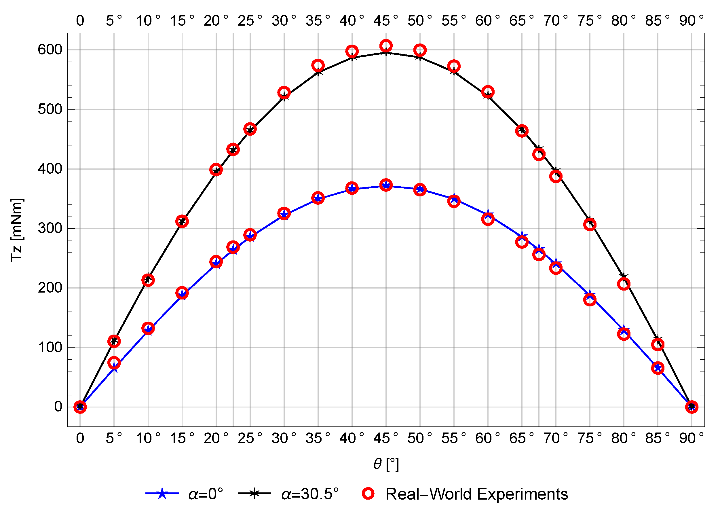
. Now, this will be studied in detail. When
° we have classical magnetic couplings (parallel rotors axes), where
is true. In this condition, if
° (null magnetic spring torque), the magnet faces of a rotor are parallels to those of the other rotor, with the same air gap between all exposed faces of magnets. Hence, the attraction and repulsion forces between magnets around the reconfiguration axis
(servomotor axis) are balanced, and there is no torque around this axis. However, the
° configuration is completely unstable because if
° (even with a small
) the attraction force between magnets (4) and (8) is greater than the force between magnets (2) and (6), thus there is a torque around axis
, which tends to increase
. In this case, to keep and control
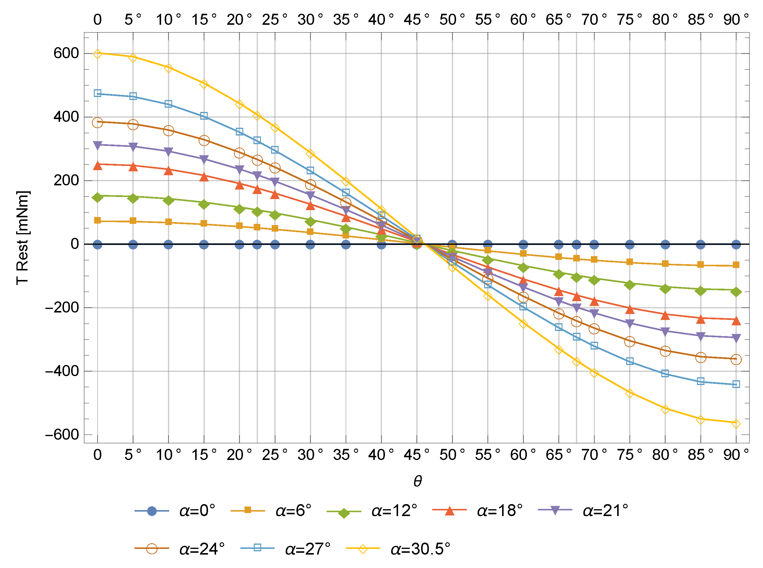
, the servomotor (
Figure 1) has to apply a counter torque, which is called
restoring torque in
Figure 2 (
in [
18]), defined by Equation (
2). Finally, due the symmetry around
axis, it is enough to calculate it with positive values of
since
.
3. Magnetostatic Numerical Modeling
The magnetostatic numerical model is implemented using the finite volume integral method [
20], from the RADIA [
21] tool. RADIA works as a library (add-on) for the Mathematica
TM [
22] software, which calls the solver, receives the results, and manages the optimization process if necessary.
The main idea of the method is to represent a magnetic body by polyhedrons (finite volumes) where the magnetization is considered uniform. Both hard (magnets) and soft (iron) magnetic bodies are represented by these volumes, and their magnetization vectors are determined as a function of the magnetic field strength . This relation can be linear for isotropic (e.g., paramagnetic and diamagnetic) and anisotropic (e.g., permanent magnets) materials, or nonlinear for other isotropic materials (e.g., ’iron’). Thus, as happens in the real world, the magnets, coils and other determined external fields (the sources of ) magnetize the soft magnetic bodies (reorienting their magnetic domains) , which interact mutually since more magnetization generates more magnetic field . Therefore, an iterative relaxation procedure is needed to evaluate how every volume magnetization affects, and is affected by, each other volume, until a stable state be achieved: . After this step, the magnetic field and field integrals can be calculated by summing the field generated by every discrete volume with its stabilized magnetization vector. The magnetic field is calculated by analytic expressions (surface integral). Using analytical formulas, it is not necessary to apply a mesh outside the bodies to know the magnetic field in free space, which reduces the processing time. This is an important difference compared to the finite element method and justifies our choice since the Flat-RMCT analysis requires many simulations.
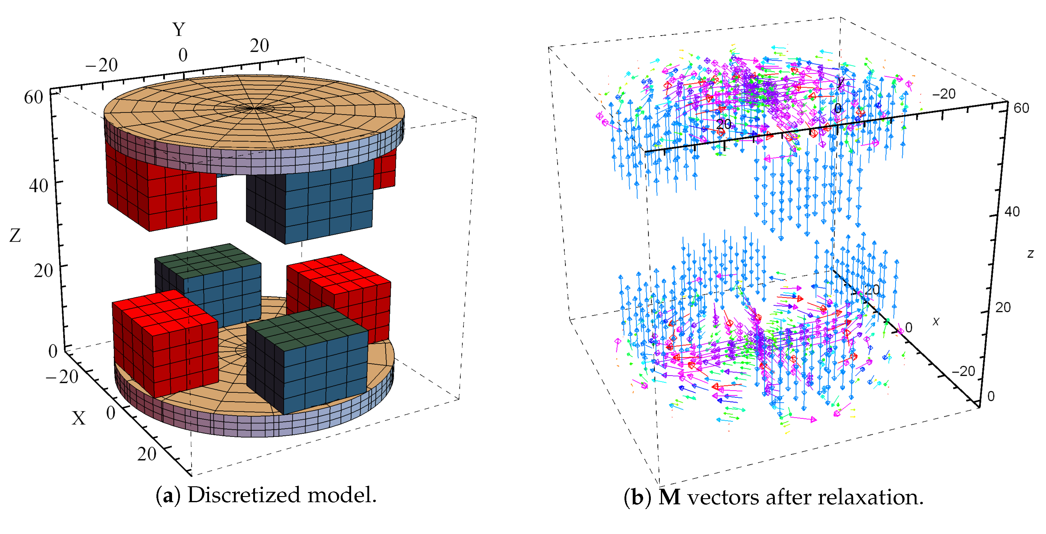
Figure 4a presents the Flat-RMCT RADIA discretized model. Each magnet is discretized in 64 parts (parallelepipeds) with constant magnetization, and each soft-iron yoke is divided into 384 elements (polyhedrons). The soft-iron yokes made of steel Z8C17 are modeled with a nonlinear magnetization behavior, using another equivalent material: 430 stainless steel. Its
curve is available at FEMM materials library [
30].
Figure 4b shows the magnetizations vectors for every polyhedron after the relaxation process.
Finally, the magnetic torque is calculated by the RADIA virtual work approach.
5. Discussion
Equations (
5) and (
6) with Equations (
8) and (
9) give us the complete model for
and
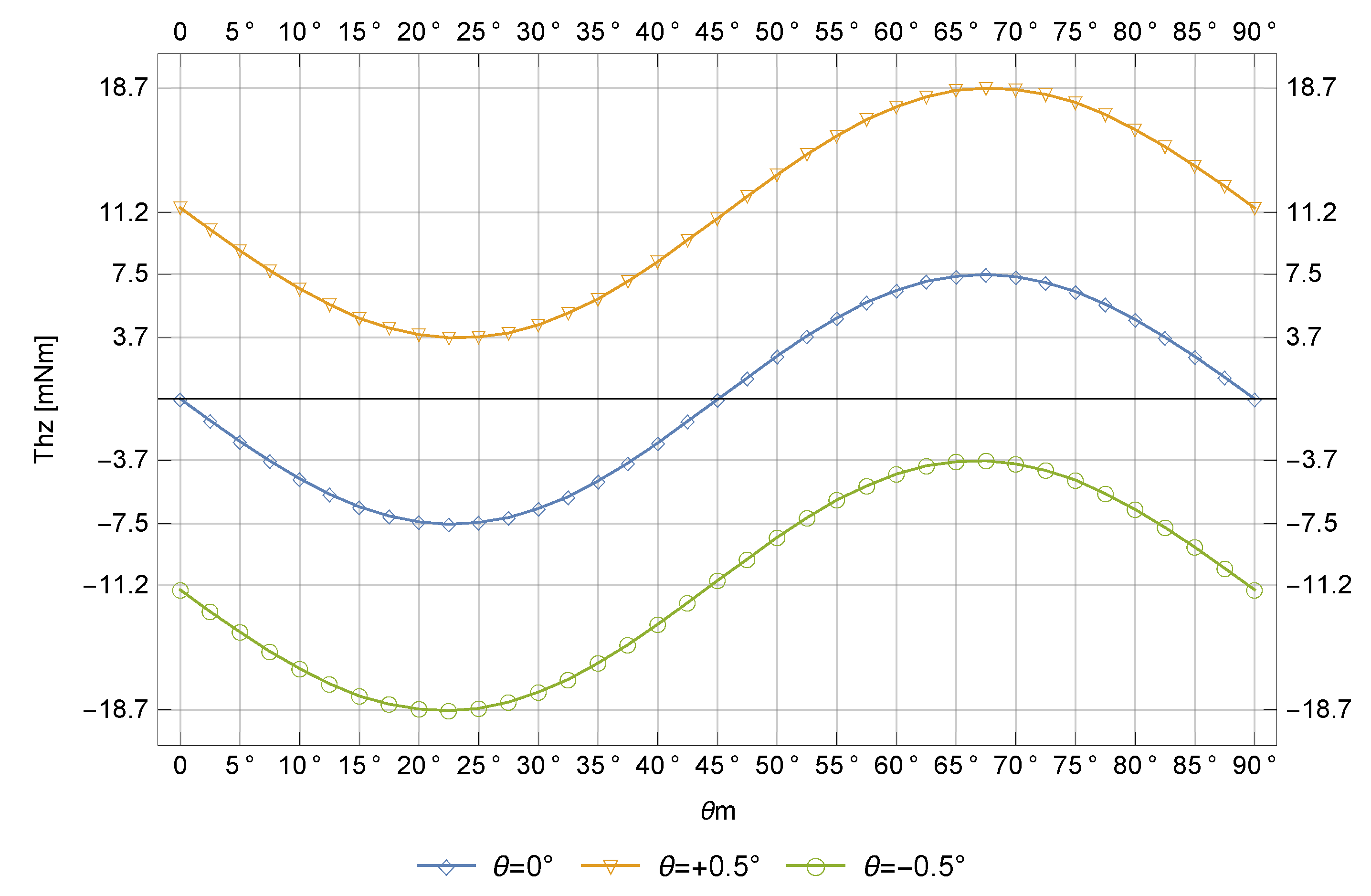
, taking into account magnetic spring and auto-driving effects. With this model, we can study the impact of the auto-driving effect on the rotors torque (when
, see
Figure 7). In work [
18], we assumed that the rotors torque was depending only on the relative position between rotors (i.e.,
) from the well-known magnetic spring effect
. Now, the auto-driving effect
depends on the absolute position of rotors (i.e.,
and
in Equations (
5) and (
6)). The consequence of
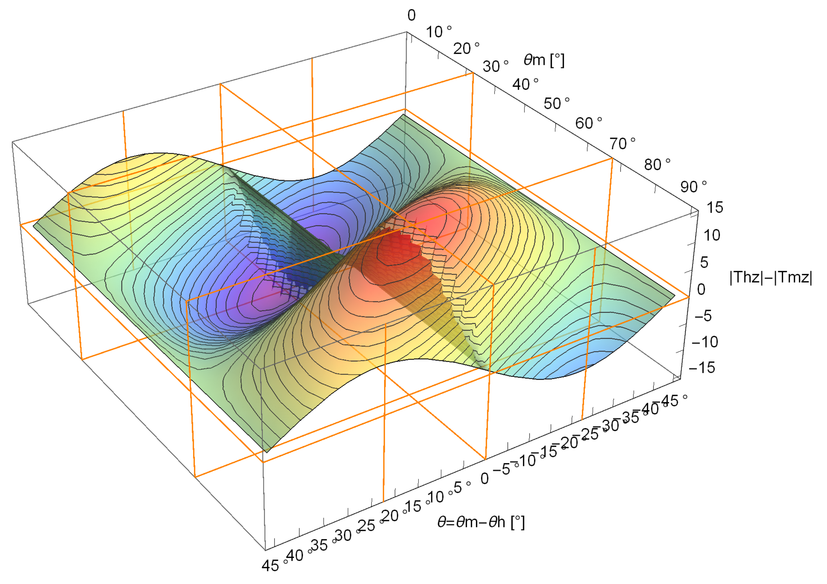
can be analyzed from the rotors torque absolute difference
.
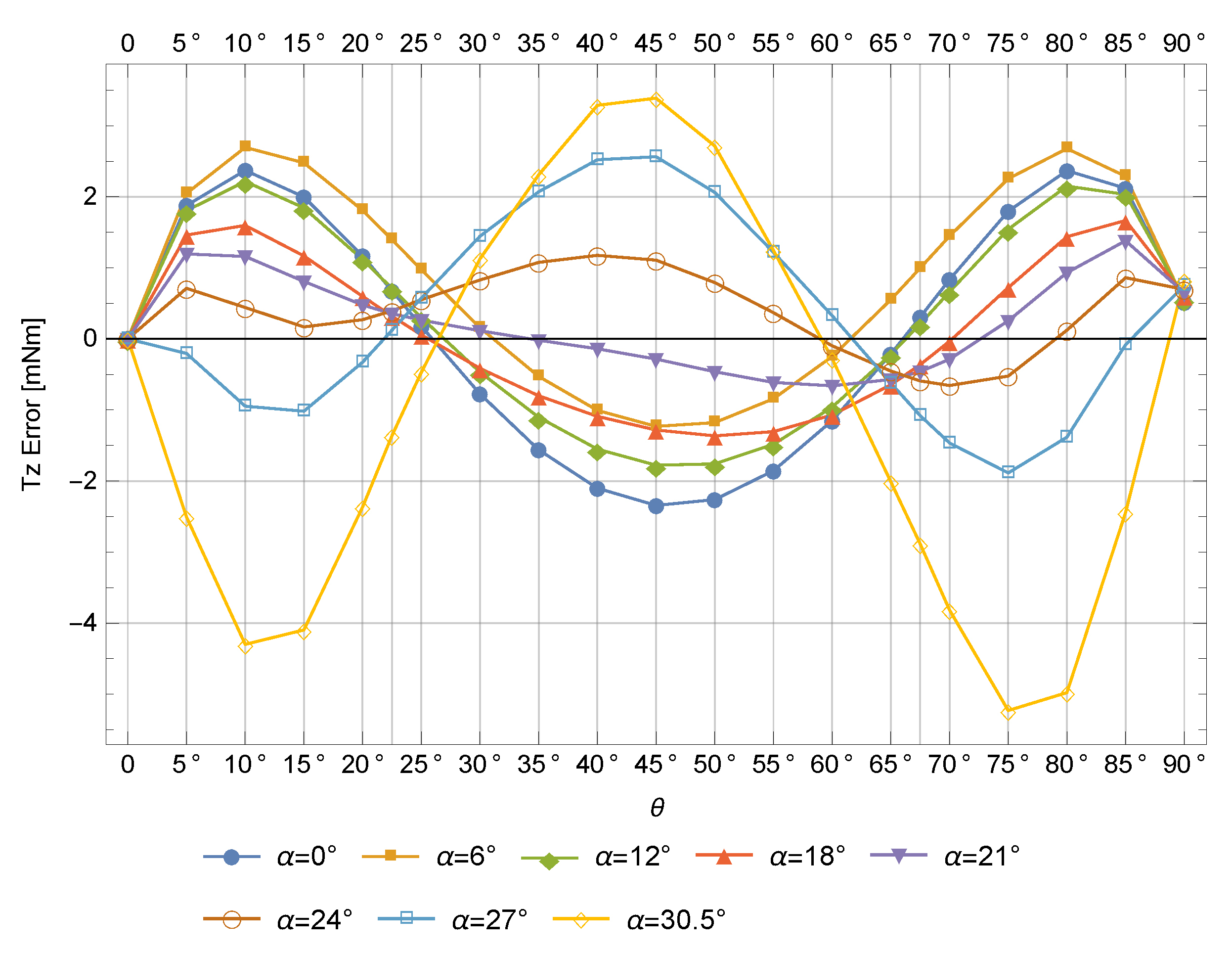
Figure 13 shows it for
, in the
operative range and for one cycle of
. Firstly, we see that the difference has an oscillatory behavior according to
and
, it is equal to zero for
and decreases when
tends towards
.
Looking into Equations (
5) and (
6) it is possible to see that
is equal to
if
, where the symmetrical rotors have their magnets oppositely equidistant from the symmetric plan. It happens also for other
and
when
. This observation has been verified with the numerical model. For example, for
and
(
) the simulation results are
and
. In addition, for
and
(also with
but with
and
shifted by 45°) the simulation results are
and
. In both cases we can consider that
, since
is the torque calculation error of our numerical model. It validates our analytical model.
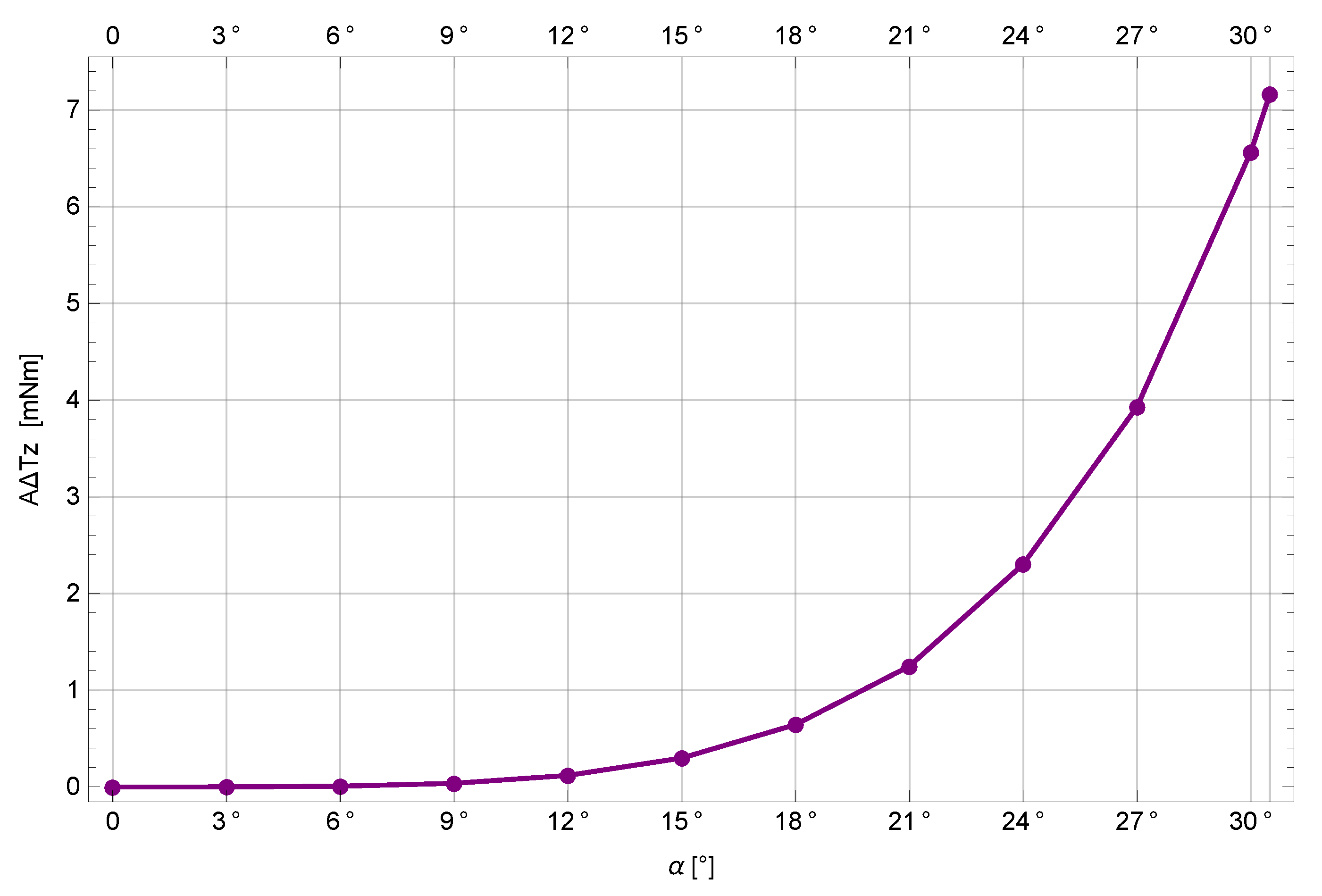
Still noting in Equations (
5) and (
6) that auto-driving and magnetic spring effects have same signs for
and opposite ones for
, the biggest difference between
and
(
, see
Figure 13) happens when the auto-driving effect absolute value is maximum and equal to the magnetic spring effect absolute value
. We have observed it for a small magnetic spring angle
, with
. We have compared this analytical model result with simulations. Where for
the analytical model gives us
and
, simulations give
and
. The difference of
is again equal to the torque calculation error of our numerical model. It also validates our analytical model.
Normally, a difference of
between motor and propeller side rotors should not be a problem. For example, if we consider that the coupling is working with
and with
of its torque transmission capacity (i.e.,
with
—see
Figure 9),
means only
of the transmitted torque.
is considered since the magnetic coupling should be designed to work close to the maximum transmissible torque, to be able to uncouple in case of load peak.
Recently, we have proposed a new reconfigurable magnetic coupling [
17], which is at least geometrically axisymmetric (i.e., composed by arc shaped magnets), tending to remove the auto-driving effect.

 ,
, 


