Abstract
Smart energy meters supporting bidirectional data communication enable novel remote error monitoring applications. This research targets characterization of the systematic worst-case error of the previously published remote watthour meter’s gain estimation method based on the comparison of synchronous measurements by the reference and meter under test. To achieve the research aim a methodology based on global maximization of the systematic error objective function assuming the typical low voltage electrical distribution network operation parameters ranges as defined by the standard recommendations for network design. To cross verify the reliability of the assessed solutions the suggested error analysis methodology was implemented utilizing two stochastic global extremum search techniques (genetic algorithms, pattern search) and the third one utilizing nonlinear programming solver. It was determined that the wattmeter adjustment gain worst-case error does not exceed 0.5% if the remote wattmeter monitored load power factor is larger than 0.1 and a network is designed according to the recommendation of the acceptable voltage drop less than 5%. For a load exhibiting power factor larger than 0.9 the worst-case error was found to be less than 0.1%. It is concluded therefore that considering the systematic worst-case error the previously suggested remote wattmeter adjustment gain estimation method is suitable for remote error monitoring of Class 2 and Class 1 wattmeters.
1. Introduction
The increasing amount of distributed electrical energy generation, smart revenue and subaccounting meters, interconnected via the advanced measurement infrastructure (bidirectional data communication channels between meters and data collection modules) are the key features of the evolving modern smart electrical grids. The demand the metrological reliability of the readings (trusted metering) of measurement devices cannot be underestimated. Not only it is crucial for maintaining the correct energy consumption billing (revenue metering) but also provides the electricity consumer with their energy consumption budget (submetering, home automation, etc.) which on its way enables changing the energy consumption behavior towards better energy efficiency of buildings, logistics, manufacturing processes, etc. The revenue metering (Level 2 in Figure 1) is a traditional level of measurement infrastructure of monitoring the energy consumption. The last decade is marked with a significant shift towards replacing the electro-mechanical meters with smart electronic meters featuring various communication capabilities. Also, the sub-accounting meters, home automation or industrial meters (Level 3) are becoming more and more popular and affordable, especially in the context of the IoT framework. Check or sum metering (Level 1) is perhaps the least deployed and not a mandatory level in monitoring energy flows especially in the low voltage electrical distribution grids. It is evident from Figure 1 that energy measurement is flowing from the network transformer towards consumers is measured twice, for example, M1-1 measures the sum of energies measured by meters M2-1, M2-2 and M2-3, M2-2 measures the sum of energies measured by meters M3-1, M3-2 and M3-3. This circumstance enables to implement the innovative methods for cross verification of the smart electricity meters. The proposed method is based on the synchronized power consumption measurements and their delivery to a smart reference meter for processing according to equations of the method. For example, in the patent [1], a method for simultaneous verification of all meters connected down to the sum meter was proposed. Also, in the paper [2] a method of simultaneous calibration of home automation smart meter’s current channel using the trusted master meter was discussed. Both methods assume that all loads consuming power are monitored by individual meters.
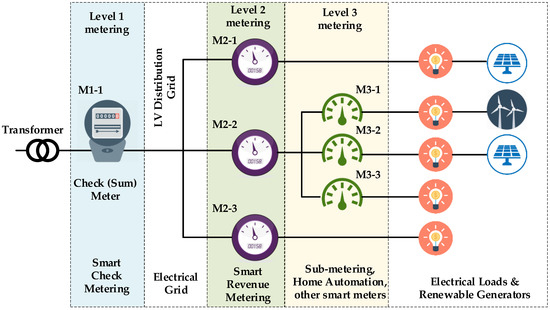
Figure 1.
Classification of power meters’ installation levels in the smart electrical grid.
A new method for remote estimation of energy meter’s adjustment factor was proposed in [3]. This method is aimed to determine the multiplicative correction factor for a separate energy meter using a remote reference energy meter. This method can be applied for verification of the selected meter despite the presence of any other power consumption occurrences by the same grid loads. The meter under inspection (later in the paper called remote wattmeter RemW) and the reference meter are installed in the electrical grid in such a way that the reference meter (later in the paper called reference wattmeter RefW) is able to measure energy consumption of the part of electrical grid including the electrical load monitored by RemW (Figure 2). The data delivery and measurement synchronization are mandatory between RefW and RemW, and a reasonably small (around 10 W) switchable verification load has to be built into the RemM or connected as an external add-on module.
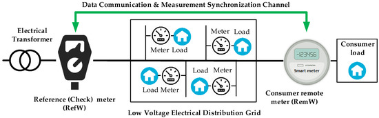
Figure 2.
Method for remote verification of electrical energy smart meters [3].
During the derivation of the RemW adjustment gain, certain assumptions influencing the systematic error of the coefficient estimation are made. These assumptions are related to the parameters of the electrical grid interconnecting RemW and RefW. The systematic error of the estimation was not yet investigated for wide range of electrical distribution networks. Usually, it is of interest to explore the worst-case error (WCE) possible in the real world electrical grid for any newly proposed measurement method. By specifying the WCE despite the electrical grid configuration and load parameters it is possible to identify the applicability of the method for remote verification of the energy meters. The real electrical grid is designed according to various recommendations and regulations. Therefore, the set of parameters characterizing real operating conditions of the network and connected loads always vary within some bounds. Derivation of analytical expression of the error as a function of grid and load parameters is a complex task because of various possible grid topologies and load characteristics including active and reactive components, harmonic distortion, etc. Even though, it might be possible to derive an analytical expression of the error but searching for the maximum WCE value and the corresponding set of grid and load parameters might be a challenging nonlinear constrained optimization task.
The goal of the research presented hereain is to determine the systematic WCE of an energy meter’s remote adjustment gain estimation procedure according to the method described in [3]. The other constituent of the total error is a random error, which was already partially explored in [3,4]. The idea of a remote watthour meter’s online adjustment gain estimation method [3] is quite new and dependence of its systematic error on circuit parameters is not investigated yet. Field calibration-based methods [5,6,7] utilize portable calibrators directly connectable to units under calibration and the calibration procedure is executed offline, i.e., with a disconnected user loads. Impedance between calibration unit and portable calibrator is small and is neglected. Specifics of the investigated remote online adjustment gain estimation method is that some irrefutable impedance separates a reference unit RefW and unit under adjustment RemW. Furthermore, if an adjustment gain evaluation procedure is carried out online, the error of the procedure is also a function of the connected loads’ size and type. There are some contributions to solve similar problems presented by other researches. G. B. Samson et al. proposed an online auto-calibration technique of system for energy consumption measurement based on low price but low accuracy Hall effect sensors (HES) [2]. Sensors for monitoring all loads connected to the household grid are installed at outputs of each breaker. The sensors are calibrated according to measurements of a single high precision current transformer installed at the main power line. To improve accuracy of the entire HES network a least mean square algorithm was applied to adjust the gain of each HES sensor in the network. The authors present comparative analysis of HES sensors network error with and without calibration for particular loads connected, i.e., three common residential appliances. Results of MATLAB simulation for the case with a higher number of sensors were also presented but detailed analysis of error dependence on system load types and magnitudes were omitted. Furthermore, the procedure proposed [2] differs in nature from the procedure introduced by authors in [3] and later explored in our work presented in the publication.
Since an evaluation of all possible combinations of external loads (types, magnitudes and power factors) in our research is costly to implement using physical models, a numerical simulation was applied. Whereas a problem is to find an extremum value for the defined bounds of parameters, the problem could be treated as a multi-parameter optimization task with non–linear constrains and parameter bounds. The genetic algorithms (GA) are often used to solve this type of optimization problems, including those coming from electric power system field. The Nonintrusive Load Monitoring system (NILM) approach based on genetic algorithms [8] can be considered as an example. The NILM [9,10,11,12] method is meant to disaggregate the consumption of the entire active power measured by standard digital watt-hour meter into its major electrical loads. GAs together with the support vector machines are the main tools of the proposed framework [13], allowing to detect any abnormal consumer behavior in the power distribution sector and identify probable power grid frauds. Other groups of power systems problems to solve using the GA are the energy consumption optimization tasks [14,15] and optimizations for forecasting purposes [16,17]. The nature of the problem under consideration is very similar to the optimal power flow [18], optimal automation devices [19] or distributed generation sources [20] allocation, optimal operating and scheduling of micro grids [21] and other problems [22,23] but with different objective functions. These are the entire tasks based on network operation mode calculations with the pre-defined non-linear constraints to find global extremum, i.e., the minimal losses, the minimal or the maximal flows, the minimal investments, or the worst-case error for the case under consideration.
The main contribution by authors in this publication is the estimation of WCE of remote gain adjustment estimation method [3] by means of solving the global nonlinear optimization problem using three different solvers for cross verification of the results reliability. The objective function for the error maximization was also composed twofold and each optimization problem separately solved by three different in nature optimization techniques, namely genetic algorithm, pattern search and nonlinear optimizer FMINCON. First, the analytical expression of the objective function was derived and used to find the WCE and electrical grid (wiring losses) and load parameters (active power, power factor). Second, the objective function was implemented using a Simulink model which was called by the used optimizers in each iteration step. The second approach is more universal, because any electrical grid configuration or load models can be applied in the WCE analysis. However, it imposes much higher requirements upon computational resources compared to analytically expressed objective function as reported in the comparative analysis contributed by the authors.
This work is structured as follows: Section 2 presents the description of the researched remote energy meter adjustment gain estimation method and its systematic error analysis; Section 3 presents the proposed methodology; Section 4 presents the method’s systematic error estimation results obtained by several methods described in the Section 3.
2. A Method for Remote Estimation of Energy Meter Adjustment Gain
2.1. Method Description and Assumptions
A method for remote wattmeter active power adjustment gain estimation was introduced in [3]. The key assumptions made for the method equations derivation are:
- It is possible to temporarily (1 s) switch on and off a small active power load (stimulus) at the location of RemW,
- Synchronized active power readings can be acquired by RefW and RemW during stimulus switching and delivered to RefW via a communication channel,
- Change of power losses and voltage drop due to stimulus state (on or off) are negligible considering 1% target error of the adjustment gain estimation,
- All network loads measured by RefW and RemW are constant during the acquisition of active powers.
The aim of the method is to determine an estimate of active power adjustment gain of the RemW. The definition of the power adjustment gain is:
where is the actual power and is the indication of active power by the RemW.
The methodology of the method development is based on some later stated assumptions followed by the derivation of expression for the adjustment gain. Afterwards, the adequacy of the made assumptions is verified by estimating systematic error. If the error is found to fall in to the acceptable range, then it is confirmed that the method is valid in the specified range of electrical network and load parameters. In this research authors focused on the analysis of the systematic WCE due to the assumptions made in the derivation of the remote adjustment gain expression.
A network model including wattmeters RefW and RemW, input energy source U1, consumer load Load 3, network loads Load 1 and Load 2, Wiring between RefW and RemW, and stimulus load PS are shown in Figure 3. Complex powers of each load and losses are denoted by S, active power by P, and reactive power by Q.
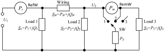
Figure 3.
A network model for the explanation of the remote wattmeter adjustment gain estimation procedure.
Active power at the connection point of the reference wattmeter (RefW) could be decomposed to the sum of network load powers and network wiring loss power for each SW (Figure 3) position:
where are powers at the point of RefW corresponding to switch SW position. The active powers are the powers of the corresponding loads (Load 1, Load 2, Load 3). In Equations (2)–(3) used notation k is used to indicate load location according to the schematics in Figure 3, while m is used to indicate position of the switch SW. is a grid wiring power loss when the load is disconnected. is the increase of network wiring active power losses due to connection of the :
are the differences of corresponding powers caused by the voltage change due to connection and disconnection of :
where the voltage difference is caused by voltage losses in network wiring due injection of load power .
Powers that should be measured by the RemW for each switch SW position can be expressed:
where are the powers at the connection point of RemW for corresponding switch SW position (Figure 3). Having unadjusted indications of the RemW wattmeter , , and considering Equation (1) the following expressions can be written:
Substituting Equations (11)–(13) to Equations (2)–(4) it is possible to rewrite:
The main assumption of the method described in [3] is that , and are constant during the remote adjustment gain estimation procedure. Therefore, these assumptions are described as:
Based on the experimental data collected from typical buildings (office, multi-apartment block, private house), it was shown in [4] that this assumption is valid with a high probability, for instance, it is 90% probability that active power consumption is fluctuations are within 1% from its nominal value during the period of 3 s.
The second assumption of the method [3] is expresed by the approximation:
The assumption (18) is equivalent to the following approximations:
The assumption (19) introduces a systematic error of the adjustement gain estimate according to the proposed method. Its impact on the systematic error is analyzed in detail aiming to verify if the assumption (19) forced errors to exceed the target level. To say in advance, it is shown at the end of the paper that even with the assumption (19) the adjustment gain estimation systematic errors stay within the level suitable to remotely monitor errors of Class 1 and Class 2 meters.
According to schematics in Figure 3 and neglecting the influence of RemW internal power losses the following equality is valid:
By subtracting both equality sides of (15) from both sides of equality (14) and taking into consideration (17), (18) and (20) it can be derived:
Power indications of RemW and are related to actual powers and by gain coefficient :
Because the method of remote adjustment gain estimation relies on the accuracy of RefW, its power indications and are assumed to be equal to the real (measured) power values, i.e.,:
To calculate according to Equation (21) only unadjusted wattmeter indications are available. Therefore, from substituting (22)–(25) to (21) it can be rewritten:
The relative error of the wattmeter adjustment gain is defined by:
Substituting Equation (26) to (27) it is possible to reduce the latter to:
2.2. Analytical Expression of Relative Error
In this section we seek to derive an analytical expression relating to network wiring and wattmeter load parameters. In [3] it was shown that losses in the internal resistance of a wattmeter RemW due to the current sensing shunt resistance (a typical value is ) are negligible because the equivalent resistance of Load 3 is many times larger. For example, 10 kW active power load in 230 V AC grid corresponds to around and increases with lower active powers. Regarding the fact that the internal impedance of a wattmeter could be neglected, the loads Load 2 and Load 3 could be considered as connected to the same potential point of the circuit. Therefore, both loads could be replaced by equivalent load:
The replacement (29) does not influence operation mode of the remaining part of the circuit, i.e., it does not influence and Let us denote the sum of Load 2 and Load 3 active powers:
and the correspondingly the change of it due to the change of voltage by:
The results of numerator and the denominator of (28) are indifferent to the connection point of the Load 2. Indeed, considering (2), (4), (8), (9), (17), (30), and (31) when the Load 2 is connected in front of the wattmeter:
and when the Load 2 is connected behind of the wattmeter:
Since the replacement of loads Load 2 and Load 3 with an equivalent load does not affect the error expression (28) and Load 1 does not influence any of the component in equations (32)–(35), the equivalent circuit shown in Figure 4 is later used for the derivation of analytical expression of . The load is modeled by a serial connection of resistive, inductive and capacitive components, while wiring impedance is modeled by a serial connection of resistance and inductance.
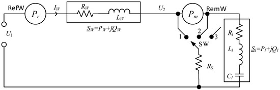
Figure 4.
Reduced network model for the explanation of the analytical error expression derivation.
By substituting (36), (38), (39), (40), and (17) to (28) the analytical expression for the relative error can be derived:
By denoting:
Equation (42) can be rewritten:
Denoting the wiring loss in the case of SW position 1 or 2 ( is connected) by , the following expression is written:
Then Equation (43) can be rewritten as:
The admittance of the overall circuit for the switch SW in position 3, could be expressed as:
The admittance of the overall circuit for the switch SW in position 1 or 2 could be expressed as:
The equivalent conductance of load and switching resistor is:
The equivalent susceptances of load and switching resistor is:
Recalculating and to series connected resistance and reactance yields:
The current through a network wiring in the case of SW position 3 according to Ohms law is:
and in the case of SW position 1 or 2 it is:
The difference of power losses in wiring with a connected and disconnected is:
The second error component in (45) caused by a difference with a connected and disconnected could be expressed by:
Voltage at the input of RemW when SW is at the position 3 ( is disconnected) could be expressed using the vector diagram method:
Voltage on the consumer side when is connected could be expressed as:
where is the phase angle between voltage and current :
and is a phase angle between voltage and current :
The power of load without connected and disconnected are correspondingly:
Then the difference of consumer power with a connected and disconnected can be expressed as:
The power difference expressed as a function of circuit parameters and voltage :
Power consumed by in the denominator of the (42)–(44) is:
Substitution of (56), (65) and (66) to the Equation (42) provides the expression of the error as a function of circuit parameters:
The analytical expression (67) can be used to find the worst-case error and the corresponding combination of network parameters. However, deriving the analytical expression for the maximum of is difficult due to the group of influencing parameters , , , , , , , . Moreover, it is necessary to describe constraints of network operation mode, restricting parameters like voltage in every point of the network, current ratings in the wiring, etc. The complexity of the problem related to the multi-parameter optimization in circuits with multiple operation mode constraints and parameter bounds yielded to the choice of its solution applying numerical optimization methods.
3. Research Methodology
3.1. Objective Functions, Constraints and Bounds of Independent Parameters
In this research we seek to determine the systematic worst-case error (WCE) of the method described in [3], considering a low voltage electrical distribution grid design and operation mode constraints. The value of is important for the judgement about the precision and applicability of the method, while the parameters of grid and loads corresponding to the WCE are important for searching the improvement of the method precision. In [3], a wattmeter adjustment gain estimation uncertainty was preliminary explored by analyzing its random and systematic components. However, the systematic error was sampled only for some specific combinations of network and load parameters that were expected to cause the largest errors. In the current publication the search of the WCE is approached by utilizing global optimization techniques, that are perform extremum (WCE) location over the whole possible range of independent parameters. Because the method introduced in [3] is very new, its systematic WCE analysis is still absent.
The objective function used to find WCE of is defined in (68), constraints function in (69) and parameter bounds in (70):
where input vector represents electrical parameters (R,L,C) of grid wiring and loads. Inequality (69) represents nonlinear constraints. In particular, includes maximum rated current through the wiring (Figure 4) and the maximum rated consumer power . Inequality (70) represents bounds of input parameters. is the vector representing the minimal possible values of circuit parameters. is the vector representing the largest acceptable values of circuit parameters.
The implementation of the optimization procedure is presented by the flowchart in Figure 5. The procedure of the input vector initialization is called randomPopulation(p_s) (Figure 5).
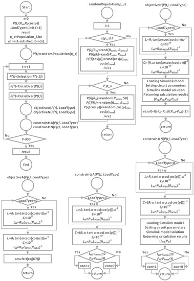
Figure 5.
Flowchart of the optimization algorithm (GA case).
In the following research the objective and constraint functions are implemented either using derived analytical error expressions (67) or by simulating a Simulink model shown in Figure 6. The second approach does not require analytical expression of the objective function and any grid can be modeled. The advantage of the second approach is that it can be easily adapted to find the worst-case error for a particular circuit. The drawback on the second approach is that the problem assigned is challenging in terms of computing requirements. Flow chart of the optimization by using genetic algorithm for both approaches presented in Figure 5. Both methods use the same logic except for calculation of the objective and constraint functions. Each time when the objective and constraint functions are called from the optimization algorithm, the first method calculates values of the objective and constraint functions applying the derived expressions. The second approach loads Simulink models, sets up network parameters of the models, solves the models, calculates and returns results of objective and constraint functions. To compute the result of the objective function, the Simulink model is solved twice. To reduce the computational load a single model corresponding SW1 and SW2 switch cases with two power measurement blocks for remote wattmeter powers and calculation is applied. To compute parameters of the constraint, function the Simulink model is solved once (SW1 case). Afterwards, the model with a circuit where the load is disconnected is called out (SW3 case). Implementation of the objective and constraint functions utilizing Simulink model are called objectiveN(P(t), LoadType) and constraintsN(P(t), LoadType). Correspondingly, the objective and constraint functions implementations utilizing analytical expressions are called objectiveA(P(t), LoadType) and constraintsA(P(t), LoadType).
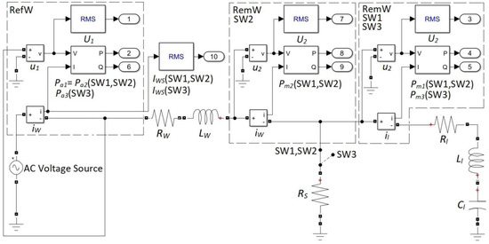
Figure 6.
Simulink model for evaluation of objective and constraint functions.
3.2. Digital Optimization Techniques
The optimization problem stated in this paper was never solved before and a priori knowledge about the objective function local and global extremums is absent. Therefore, to cross verify the obtained solutions several strongly different optimization techniques should be employed. Also, it is obvious that the optimization problem is nonlinear, multivariable, and includes nonlinear constraints. genetic algorithm (GA), pattern search (PS) methods and nonlinear programing solver FMINCON [24] were selected to conduct the WCE search. Key features and their fit to the solution of the stated optimization problem are shortly summarized below.
The GA is a stochastic optimization method based on Darwin’s theory of natural selection and the mechanism of population genetics. It initializes the first population randomly and through a process of evolution tends to find the most fit individual, i.e., combination of input parameter values that correspond to the maximum (minimum) value of the objective function. Each new generation produced by selection, crossover and mutation operators. GA method was successfully applied to solve nature related problems just for different goals [25]. The GA method is easy adaptable for a particular problem, does not require prioritization, scale, or weight objectives, and is an attractive alternative to other optimization methods because of its robustness in finding global optimum. Since the input values of the GA are taken recursively, the algorithm operates purposefully and, in many cases, would give the result faster in comparison to pure random search (PRS) or Monte Carlo simulation where inputs are chosen in purely random manner. Speed of an algorithm convergence is important for the problem because calculation of the objective function is time consuming especially for Simulink-based approach.
To verify the obtained solutions, the pattern search (PS) method is used in our research. PS is a derivative-free algorithm of a class of direct search (DS) methods for solving optimization problems [26]. The algorithm recursively searches a set of points around the current point, so called mesh, to find closer to optimum (lower/higher) value of objective function in each iteration. The mesh formed in the previous iteration by adding the current point to a scalar of vectors is called a pattern [26]. If the mesh improves the objective function of the current point, it becomes the new point, otherwise, the new mesh is formed, and calculations are repeated. The procedure is iterated until stopping criteria is met. A stand-alone PS algorithm tends to fall into local minima (maxima) [27]. According to the method application recommendations [27] to find the global extremum, multiple starting points were defined and implemented. The points are initiated in a random way from the defined parameter bounds. Half of the points are initiated for a set of parameters with a higher probability of an optimum point. Estimation of ranges of the higher optimum point probability are presented further in the section “Parameter Bounds”. The DS methods as GA were successfully applied for some power system optimization tasks also [28,29].
Nonlinear programing solver FMINCON based on the interior point algorithm was the third optimization method implemented for problem solving. FMINCON is a solver used to find the minimum of the constrained multivariable function [24]. Contrary to the first two methods it is a gradient-based method that is designed to work on problems where the objective and constraint functions are both continuous and have continuous first order derivatives [24]. As well as PS, the FMINCON was utilized to search for the extremum point from set of different starting points. A fraction of them was chosen from region of higher probability of the optimum point.
Usually optimization solvers are designed to search for an objective function minimum. However, according to the definition of WCE in Equation (68) it is required to find the maximum of the objective function. Therefore, the objective function is transformed into the inverse function:
Implementation cost and complexity of GA, PS and FMINCON are not considered in this publication because MATLAB toolboxes were used in research. Objective and constraints functions were implemented in MATLAB script language according to Equations (28), (67) and (75) and related expressions.
3.3. Simulation Settings
3.3.1. Electrical Parameters Calculation
The input parameters of the objective function are: load resistance , wire resistance and the load power factor . Since the inductive and capacitive loads have the opposite signs of reactance, there is an infinite amount of possible combinations of inductance and capacitance that meet particular load power factor for the fixed value. Therefore, submission of the load inductance and capacitance to objective function as input parameters are fated to poor convergence of the solution. Therefore, the power factor was chosen as an input parameter to define the reactive load. While the linear loads could be or type, separate GA searches were established for both cases allowing just type load for one case and just for another. Parameters and are calculated inside of the objective function from the resistance and according to the following formulas:
where is angular frequency. Expressions (72) were used for the case of type load, while expressions (73) for the case of type load. Inductance of the wiring cable is calculated inside of the objective function according to expression:
where is a resistance of 1 meter cable length, is 1 meter inductance of the same cable.
Expressions (72)–(74) were used to calculate load and wiring electrical parameters in the optimization algorithm explained in Figure 5.
3.3.2. Nonlinear Inequality Constraints
The used nonlinear inequality constraints denoted in Equation (69) are:
Load resistance , wire resistance and load power factor are the input parameters of the constraint function (75) as well as for the objective function. Parameters , and are calculated by applying formulas (72)–(74). When the analytical expression of the objective function is used, the value is calculated by applying the Equation (55). Calculation of value is defined in Equation (63). When Simulink model (Figure 6) is used, the and are estimated by solving the circuit presented in Figure 4.
The current is set according to the calculated value for a particular defined maximum rated load power nominal voltage and power factor :
where is the maximal consumer active power for a particular case under consideration. A typical power factor for residential load is used in this case. The nominal voltage .
3.3.3. Parameter Bounds
Parameter bounds in (70) are vectors of a circuit and operation mode parameters defining a range of values for independent input parameters:
The upper bound of a network wiring active resistance is calculated according to the standard limits of allowable voltage drop in low voltage network. In many countries voltage drop in low voltage distribution network cannot exceed 5% [30]. Since for the fundamental frequency , the inductance of the cable could be neglected. To calculate upper bound of the wire resistance, the simplified expression is used:
The lower bound of wire active resistance is accepted to be:
Bounds for were chosen in connection to nominal network voltage and the maximum rated power measured by the RemW:
where in all of the following simulations (corresponds to ), and is specified along with the presented results in the next chapter, for example with power factor , corresponds to .
The upper power factor bound of in Equation (77) corresponds to pure active load (). The lower bound for the power factor is in the range from 0.1 to 0.9 and is dependent on the simulation settings specified in the next section.
3.3.4. Initial Points Selection
To improve a convergence to a solution, some fraction of initial population (for GA) or a fraction of initial points (for PS, FMINCON) were forced to meet the parameter ranges with higher probability of the optimum point. To determine the parameter range, the objective function was calculated by changing one parameter by fixed step for a wide range while the rest of the parameters were kept constant. The results are presented in Figure 7, Figure 8 and Figure 9.
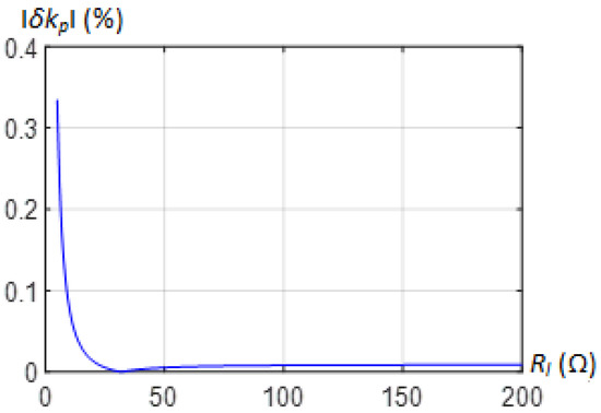
Figure 7.
Error dependence on the load resistance .
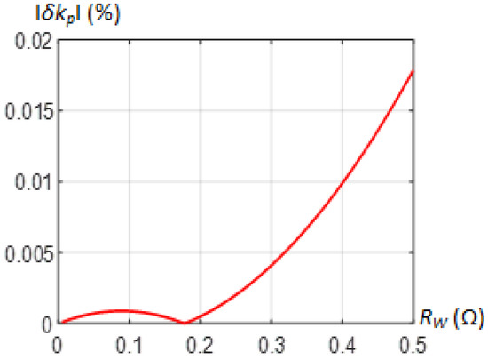
Figure 8.
Error dependence on the wiring resistance .
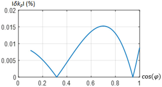
Figure 9.
Error dependence on the load power factor .
According to the results, bounds for a half of initial population defined as follows:
All members of the initial population (for GA case) or initial points (for PS, FMINCON cases) were initialized randomly. During the initialization half of the initial population (for GA) or initial points (for PS, FMINCON) were forced to meet the bounds defined by Equations (77)–(81). The second half of the initial population (initial points) was forced to meet the bounds defined in Equation (82).
4. Results and Discussion
4.1. The Network Parameters Corresponding to the Worst-Case Error
Following the aim of the research to identify the WCE and the corresponding network and load parameters, a combination of typical loads, wire resistances, and power factor values were used to search for according to Equations (68)–(70). Though the input vector in (70) is , the most often measured parameters by the metering instruments are load power and power factor . Also, a distribution network design recommendation include restrictions on power losses and transferred power ratio. The results presented in this chapter are aimed to reveal dependence on , and . The complete set of the obtained results are shown in Table 1 and Table 2, while some of dependencies are plotted graphically in Figure 10, Figure 11, Figure 12 and Figure 13.

Table 1.
Results obtained by GA and PS methods for R, RL, RC type loads.
Table 2.
The adjustment gain relative error dependence on the maximum rated load power 5 kW, 7 kW, and 10 kW.
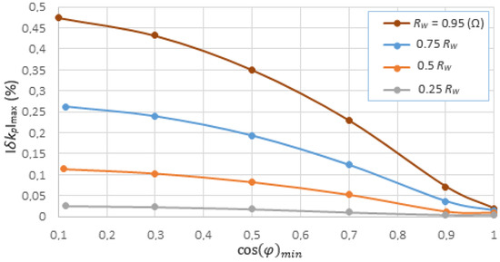
Figure 10.
The dependence of the adjustment gain error on the lower bound of load power factor and on the upper bound of wire resistance.
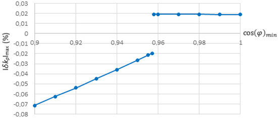
Figure 11.
Dependence of the wattmeter gain WCE on power factor in the range of a load power factor 1.
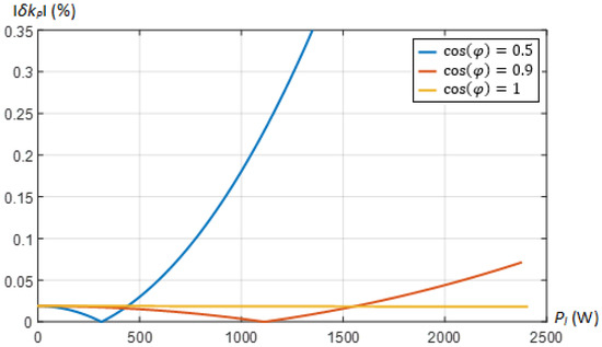
Figure 12.
Dependence of the error on load power and power factor.
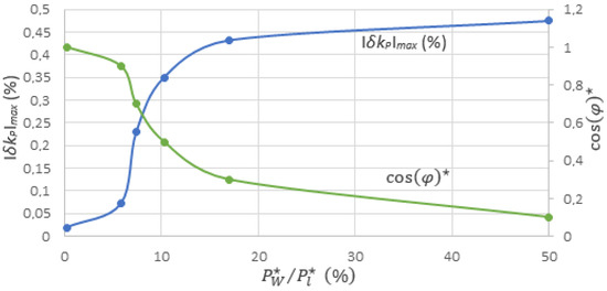
Figure 13.
Dependences of the WCE on power factor on power losses to load power ratio for the WCE.
Simulation results in the case of the maximum load power and pure active load (), active-inductive () and active-capacitive () type load are presented in Table 1. The set of selected parameters is considered as typical for the case when the reference meter is a revenue meter and the meter under adjustment is a sub-accounting meter like a smart socket in a residential apartment.
The differences of the error obtained by different in their nature search methods GA, PS and FMINCON are marginal. The differences of the error in cases of type and type load are also minor with a trend for type loads to produce slightly higher error values. The practical meaning of the differences is negligible, therefore only results of the error estimations for the more common type loads are presented further.
It is the value of WCE is the most important parameter characterizing remote adjustment gain estimation method accuracy. The same goal attained by three different search methods ensures that the global maximum was found. The possibility that there might exist yet another vector of independent variables yielding the same maximum error can only be important for understanding the worst case network configuration but does not affect the characterization of the remote estimation method.
To visualize the influence of the wiring resistance on the adjustment gain error, the GA search was completed for the upper bounds , and in addition to . The obtained results are plotted in Figure 10.
The results of presented research indicate that the WCE values were found for the highest wire impedance values . The trend of the increasing error with each increment of the wiring impedance supports the assumption that the source of the error is the wiring impedance between RefW and RemW. The assumption could be made by analyzing the Equations (36), (42), (43) and (67). Zero wiring impedance ( and ) results in zero values of both and , and according to the equation (67), consequently to . On the other hand, it could be a future research direction to estimate wiring losses on-line and look for the modification of the adjustment gain estimation method by including information about the wiring resistance or losses and expecting to reduce its WCE.
According to Table 1, the WCE in case of the active load corresponds to the smallest load (the upper bound of ), but WCE corresponds to the largest load (the lower bound of ) when To investigate the haziness a more detail exploration of WCE dependency on power factor is conducted in a range of load power factor 1 and plotted in Figure 11. The explanation to the form of the dependence in Figure 11 can be given by analyzing Equations (42)–(45). The results presented in Figure 11 show that by incrementing the minimal bound of power factor leads to reduction of the error modulus, while value always remains negative. In this range the error component related to the load power change dominates over the error component related to change of wiring losses (43). By reaching some threshold power factor , the sign of turns positive. In the range , the WCE is found corresponding to lowest load () and dominates over . Despite this discontinuity of the dependence , the modulus of as it can be seen from Table 1 and Figure 10, is always decreasing in response to increase of the load power factor .
The simulation results corresponding to are presented in Table 2. It can be seen from Table 2 that the load power factor reduction always degrades the error despite the largest allowed load power . The comparison of the results in Table 1 and Table 2 reveals that the error values are similar for the same load power factor in the whole explored the minimal power factor range (). It could be explained by the fact that the product is constant. Cable impedance must be less, while the maximal current is relatively higher for higher powers to meet the requirement of the largest allowable voltage drop (5%). Equal or lower than the allowable impedance of the wires must be assured by selecting proper diameter of wires during the electrical distribution grid design stage. The results also show that the increase of gives the same impact on results as proportional relative increase of for the power factor bounds resulting in negative error values. Summarizing up the results, it can be clearly stated that the WCE is obtained from combination of the highest wiring impedance (, ), the highest allowable current , and the lowest load power factor values.
To visualize the dependence of the error modulus on load value which is calculated according to Equation (62), the direct error value calculations are carried out using Equation (67) and Figure 12 is plotted. Figure 12 indicates that a real error in case of a particular can be significantly less than which corresponds to the maximum considered load. The real error value could be estimated by measuring and and utilizing expression approximated from data shown in Figure 12. However, since is less that the target accuracy of 1%, in the current stage of the development, we did not attempt to derive the precise error estimation but only focused on its upper limit .
In Figure 13 there are presented WCE and load power factor dependencies on power loss to load power ratio . Power loss to load power ratio is often accepted as selection criteria for power distribution grid cables. It can be seen that decreasing the power factor of a load herewith also increasing loss to load power ratio, causes the increase of the wattmeter gain estimation error. This dependence is nonlinear and if the error value is much below the 1% target. Even in the case of abnormal level of power losses in the network (Figure 4) wires, the method yields wattmeter adjustment gain estimation error less than 0.5%.
4.2. Requirements upon Computational Resources
The aim of this section is to compare the computational cost of all applied global search algorithms combined with the methods of objective function implementation. The analytical derivation of the expression of WCE is based on the mentioned approximations. In opposite, the Simulink model based objective function does not include any approximate assumptions. Therefore, it is of important to estimate if using the analytical expression is reasonable in a sense of speeding up calculations. For the case of analytically expressed objective function optimization it is of interest to discover which of algorithm (GA, PS, FMINCON) perform faster in finding the same solution. The objective function is unique because it is derived from new method equations introduced in [3]. Therefore, it was not solved by someone else and computational cost reported in the analysis below cannot be compared over data of any other references.
The obtained wattmeter adjustment gain WCE values along with calculation times and population size of GA or number of initial points of PS are presented in Table 3. All computations were performed on Dell PowerEdge R730 server with two Intel(R) Xeon(R) CPU E5-2620 v3 @ 2.40 GHz processors, together containing 12 physical cores and 24 logical cores with 32 GB operating memory. The power management profile of the computer operational system was set to performance level during the simulations. The computations were implemented and performed using MATLAB Parallel computing toolbox. The comparative speed analysis was carried out for a load power factor within the range .
Table 3.
Comparative analysis of the applied search methods.
The GA search based on objective and constraint functions implemented applying analytical expressions yielded the result much faster in comparison to Simulink based implementation of objective and constraints functions despite for the 100 times larger search population size. The higher population size caused slightly higher extremum value with much higher probability of the result being a global minimum. PS implementation applying analytical expressions gave a very close result in noticeably lower time in comparison to the same implementation of the GA method. FMINCON based search implementation of analytical expressions has shown a noticeable speed advantage in comparison to the rest methods and gave very close result as can be seen from Table 3. Therefore, the results in Table 3 support the statement, that using analytical expression does not lead to the loss of search precision but significantly reduce computational cost. Also, FMINCON seems to obtain the same solution of the optimization problem (66) several times faster than GA and PS methods.
5. Conclusions
The systematic worst-case error (WCE) of a previously introduced wattmeter adjustment gain remote estimation method was studied using the simplified electrical energy delivery model enabling to derive an analytical expression of the error (objective function) and constraint functions. To find the WCE, the error expression was maximized using two stochastic search techniques (genetic algorithm, pattern search) and the nonlinear programming solver. The adequacy of the error analytical expression and its maximization solution was verified by the second approach based on numerical simulation of electrical circuit model. Both solutions obtained produced very close results with practically insignificant differences. The second approach utilizing numerical electrical circuit model universal in a sense that it enables to find the WCE together with the corresponding electrical network configuration without analytical expression of the objective function. However, the requirements for computational cost is many times higher for the second approach. For the considered network model the computation time required to reach the solution was over 200 times longer to the search of WCE using the derived analytical expression. Therefore, it we the second approach is recommended for the verification of the correctness of problem solution, but analytical expression is reasonable for
The research has revealed that the systematic error of the method is influenced by the wattmeter monitored load active power, its power factor and losses in the network wiring between reference and wattmeter under test. It was found that the WCE is below 0.5% if the load power factor is larger than . The WCE is less than 0.1% for a load exhibiting power factor larger than in a distribution network designed following the recommendations to ensure the grid voltage magnitude drop not more than 5%. The WCE of the proposed method is a conservative characterization of error range. Therefore, the systematic error of the described remote adjustment gain estimation method does not exceed error limits of Class 2 and Class 1 watthour revenue meters.
Author Contributions
Ž.N. supervised the research and was responsible for the funding acquisition; all the authors contributed in literature review; Ž.N. and V.D. performed description of the remote adjustment gain estimation method; R.L., R.D. and R.R. done adjustment gain error analysis; R.L. developed and implemented WCE search methods and algorithms; all the authors performed the results analysis, discussion, conclusions formulation and contributed to writing the paper; P.K. was responsible for second project funding acquisition and paper language proof reading.
Funding
This research was supported by the Research, Development and Innovation Fund of Kaunas University of Technology, grants No. MTEPI-P-17026 and No. MG1706.
Conflicts of Interest
The authors declare no conflict of interest.
Nomenclature
| Abbreviations | |
| GA | genetic algorithms |
| PS | pattern search |
| DS | direct search |
| FMINCON | function for nonlinear constrained optimization [24] |
| WCE | worst-case error |
| RefW | reference wattmeter |
| RemW | remote wattmeter |
| HES | Hall effect sensors |
| SW | switch |
| SW1 | switch in position 1 |
| SW2 | switch in position 2 |
| SW3 | switch in position 3 |
| Variables | |
| kp | power adjustment gain |
| kp* | estimate of power adjustment gain |
| δkp | relative error of the wattmeter adjustment gain |
| P | active power (W) |
| P* | the indication of active power by the wattmeter under gain adjustment RemW (W) |
| ΔP | active power loss (W) |
| active power loss change due to adjustment load connection (W) | |
| active power of the ith load change due to the kth voltage change (W) | |
| Q | reactive power (Var) |
| S | complex power (VA) |
| U | voltage (V) |
| ΔU | voltage difference (V) |
| I | current (A) |
| Y | admittance (S) |
| Z | impedance (Ω) |
| R | resistance (Ω) |
| X | reactance (Ω) |
| G | conductance (S) |
| B | susceptance (S) |
| L | inductance (H) |
| C | capacitance (F) |
| load power factor | |
| vector of input parameters | |
| H | vector of constraints quantities |
| wiring current constraint | |
| active load constraint | |
| Subscripts and Superscripts | |
| r | reference wattmeter |
| m | remote wattmeter |
| W | wiring parameter |
| S | network regime with a gain adjustment load connected or parameter/quantity of the corresponding network |
| l | load parameter |
| L | inductive |
| C | capacitive |
| max | maximum |
| min | minimum |
| N | nominal |
| * | indication/estimate containing an error |
| parameter/quantity corresponding to the maximum error case | |
References
- Seppa, H. Method and System for the Calibration of Meters. WIPO Patent 063180 A1, 6 July 2007. [Google Scholar]
- Beaufort Samson, G.; Levasseur, M.; Gagnon, G.; Gagnon, F. Auto-calibration of Hall effect sensors for home energy consumption monitoring. Electron. Lett. 2014, 50, 403–405. [Google Scholar] [CrossRef]
- Nakutis, Ž.; Saunoris, M.; Ramanauskas, R.; Daunoras, V.; Lukočius, R.; Marčiulionis, P. A Method for Remote Estimation of Wattmeter’s Adjustment Gain. IEEE Trans. Instrum. Meas. 2018, 1–9. [Google Scholar] [CrossRef]
- Nakutis, Ž.; Saunoris, M.; Daunoras, V.; Lukočius, R.; Marčiulionis, P.; Deltuva, R.; Ramanauskas, R. A Short-term Power Fluctuations Averaging in Low Voltage AC Grid. In Proceedings of the IEEE International Workshop on Applied Measurements for Power Systems (AMPS), Liverpool, UK, 20–22 September 2017; pp. 1–6. [Google Scholar]
- Amicone, D.; Bernieri, A.; Ferrigno, L.; Laracca, M. A smart add-on device for the remote calibration of electrical energy meters. In Proceedings of the Instrumentation and Measurement Technology Conference, Singapore, 5–7 May 2009; pp. 1599–1604. [Google Scholar]
- Femine, A.D.; Gallo, D.; Landi, C.; Luiso, M. Advanced Instrument for Field Calibration of Electrical Energy Meters. IEEE Trans. Instrum. Meas. 2009, 58, 618–625. [Google Scholar] [CrossRef]
- Jebroni, Z.; Chadli, H.; Tidhaf, B. Remote calibration system of a smart electrical energy meter. J. Electr. Syst. 2017, 13, 806–823. [Google Scholar]
- Egarter, D.; Sobe, A.; Elmenreich, W. Evolving Non-Intrusive Load Monitoring; LNCS 7835; Springer: Heidelberg, Germany, 2013; pp. 182–191. [Google Scholar]
- Lu, H.; Xin, W.; Hui, B.; Bing, Q.; Aixia, Z. A residential load identification algorithm based on periodogram for non-intrusive load monitoring. In Proceedings of the China International Conference on Electricity Distribution (CICED), Xi’an, China, 10–13 August 2016; pp. 1–4. [Google Scholar]
- Li, H.D.; Dick, S. Residential Household Non-Intrusive Load Monitoring via Graph-Based Multi-Label Semi-Supervised Learning. IEEE Trans. Smart Grid 2018. [Google Scholar] [CrossRef]
- Tabatabaei, S.M.; Dick, S.; Xu, W. Toward Non-Intrusive Load Monitoring via Multi-Label Classification. IEEE Trans. Smart Grid 2017, 8, 26–40. [Google Scholar] [CrossRef]
- Agyeman, K.; Han, S.; Han, S. Real-Time Recognition Non-Intrusive Electrical Appliance Monitoring Algorithm for a Residential Building Energy Management System. Energies 2015, 8, 9029–9048. [Google Scholar] [CrossRef]
- Nagi, J.; Yap, K.S.; Tiong, S.K.; Ahmed, S.K.; Mohammad, A.M. Detection of abnormalities and electricity theft using genetic Support Vector Machines. In Proceedings of the TENCON 2008—2008 IEEE Region 10 Conference, Hyderabad, India, 10–21 November 2008; pp. 1–6. [Google Scholar] [CrossRef]
- Papantoniou, S.; Kolokotsa, D.; Kalaitzakis, K. Building optimization and control algorithms implemented in existing BEMS using a web based energy management and control system. Energy Build. 2015, 98, 45–55. [Google Scholar] [CrossRef]
- Ullah, I.; Kim, D. An Improved Optimization Function for Maximizing User Comfort with Minimum Energy Consumption in Smart Homes. Energies 2017, 10, 1818. [Google Scholar] [CrossRef]
- Fan, G.; Peng, L.; Zhao, X.; Hong, W. Applications of Hybrid EMD with PSO and GA for an SVR-Based Load Forecasting Model. Energies 2017, 10, 1713. [Google Scholar] [CrossRef]
- Zheng, D.; Shi, M.; Wang, Y.; Eseye, A.; Zhang, J. Day-Ahead Wind Power Forecasting Using a Two-Stage Hybrid Modeling Approach Based on SCADA and Meteorological Information and Evaluating the Impact of Input-Data Dependency on Forecasting Accuracy. Energies 2017, 10, 1988. [Google Scholar] [CrossRef]
- Asnawi, Y.; Hasannuddin, T. Voltage Constrained Optimal Power Flow Based Using Genetic Algorithm. J. Kejuruteraan 2015, 27, 9–14. [Google Scholar]
- Stojanović, M.; Tasić, D.; Ristić, A. Optimal Allocation of Distribution Automation Devices in Medium Voltage Network. Electron. Electr. Eng. 2013, 19, 9–15. [Google Scholar] [CrossRef]
- Bhullar, S.; Ghosh, S. Optimal Integration of Multi Distributed Generation Sources in Radial Distribution Networks Using a Hybrid Algorithm. Energies 2018, 11, 628. [Google Scholar] [CrossRef]
- Marzband, M.; Sumper, A.; Domínguez-García, J.S.; Gumara-Ferret, R. Experimental Validation of a Real Time Energy Management System for Microgrids in Islanded Mode Using a Local Day-Ahead Electricity Market and MINLP. Energy Convers. Manag. 2013, 76, 314–322. [Google Scholar] [CrossRef]
- Kumar, A.; Das, B.; Sharma, J. Genetic Algorithm-Based Meter Placement for Static Estimation of Harmonic Sources. IEEE Trans. Power Deliv. 2005, 20, 1088–1096. [Google Scholar] [CrossRef]
- Köse, E.; Abaci, K.; Kizmaz, H.; Aksoy, S.; Yalҫin, M. Sliding Mode Control Based on Genetic Algorithm for WSCC Systems Include of SVC. Electron. Electr. Eng. 2013, 19, 19–25. [Google Scholar] [CrossRef]
- Mathworks Documentation. Available online: https://se.mathworks.com/help/optim/ug/fmincon.html (accessed on 7 May 2018).
- Huang, P. Reactive Power Optimization Analysis of 35KV Regional Power Grid Based on the Genetic Algorithm. Adv. Mater. Res. 2014, 1055, 271–274. [Google Scholar] [CrossRef]
- Mathworks Documentation. Available online: https://se.mathworks.com/help/gads/patternsearch.html (accessed on 12 December 2018).
- MathWorks. Global Optimization Toolbox User’s Guide R2017b; The MathWorks, Inc.: Natick, MA, USA, 2017; pp. 1–18. [Google Scholar]
- Huang, W.; Yao, K.; Wu, C.; Chang, Y.; Lee, Y.; Ho, Y. A Three-Stage Optimal Approach for Power System Economic Dispatch Considering Microgrids. Energies 2016, 9, 976. [Google Scholar] [CrossRef]
- Huang, W.; Yao, K.; Wu, C. Using the Direct Search Method for Optimal Dispatch of Distributed Generation in a Medium-Voltage Microgrid. Energies 2014, 7, 8355–8373. [Google Scholar] [CrossRef]
- Electrical Installation Guide According to IEC International Standards 2016. Rueil-Malmaison (BP 50604, 92506 Cedex): Schneider Electric. Available online: https://www.schneider-electric.com/en/work/products/product-launch/electrical-installation-guide/ (accessed on 12 December 2018).
© 2018 by the authors. Licensee MDPI, Basel, Switzerland. This article is an open access article distributed under the terms and conditions of the Creative Commons Attribution (CC BY) license (http://creativecommons.org/licenses/by/4.0/).