Article

Closed-Form Solution of Radial Transport of Tracers in Porous Media Influenced by Linear Drift

by
Lateef T. Akanji
1,* and
Gabriel K. Falade
2
1
Division of Petroleum Engineering, School of Engineering, University of Aberdeen, Aberdeen AB24 3FX, UK
2
Department of Petroleum Engineering, University of Ibadan, Ibadan 23402, Nigeria
*
Author to whom correspondence should be addressed.
Energies 2019, 12(1), 29; https://doi.org/10.3390/en12010029
Submission received: 3 November 2018 / Revised: 10 December 2018 / Accepted: 17 December 2018 / Published: 22 December 2018
(This article belongs to the Special Issue Sustainability of Fossil Fuels)

Abstract

:
A new closed-form analytical solution to the radial transport of tracers in porous media under the influence of linear drift is presented. Specifically, the transport of tracers under convection–diffusion-dominated flow is considered. First, the radial transport equation was cast in the form of the Whittaker equation by defining a set of transformation relations. Then, linear drift was incorporated by considering a coordinate-independent scalar velocity field within the porous medium. A special case of low-intensity tracer injection where molecular diffusion controls tracer propagation but convection with linear velocity drift plays a significant role was presented and solved in Laplace space. Furthermore, a weak-form numerical solution of the nonlinear problem was obtained and used to analyse tracer concentration behaviour in a porous medium, where drift effects predominate and influence the flow pattern. Application in enhanced oil recovery (EOR) processes where linear drift may interfere with the flow path was also evaluated within the solution to obtain concentration profiles for different injection models. The results of the analyses indicated that the effect of linear drift on the tracer concentration profile is dependent on system heterogeneity and progressively becomes more pronounced at later times. This new solution demonstrates the necessity to consider the impact of drift on the transport of tracers, as arrival times may be significantly influenced by drift intensity.

1. Introduction

The study of the transport of tracers has become an essential technique for porous media characterisation, particularly in enhanced oil recovery (EOR) in hydrocarbon reservoirs (e.g., Baldwin [1]), hydrology (e.g., Rubin and James [2]), nuclear (e.g., Moreno et al. [3] and Herbert et al. [4]), drug transport in blood vessels (e.g., Mabuza et al. [5]) and geothermal engineering (e.g., Vetter and Zinnow [6]). Multiple processes and mechanisms are usually involved in the chemical interaction of the constituent components when the tracer is being transported through a porous medium. Two major processes involved in the transport phenomenon include convection and hydrodynamic dispersion. The convection process involves bulk movement of fluids, while hydrodynamic dispersion describes the dual actions of molecular dispersion and shear or mechanical mixing process. These complementary transport processes are adequately captured by the well-known convection–dispersion–diffusion equations with or without chemical reactions (e.g., Tomich et al. [7], Bear [8], Zhou and Zhan [9]).
Surfactant or biosurfactant partitioning and transport in the oil phase during enhanced oil recovery processes is usually neglected, because, it requires the solution of a system of nonlinear coupled partial differential equations whose solution is numerically challenging [10]. These diffusion equations are based on linear or one-dimensional geometry due to the relative ease with which such equations can be solved analytically. Recently, several authors have studied hydrodynamic transport in porous media using the random walk method (see a review paper by Noetinger et al. [11] and references cited therein). Approximate solutions have also been presented in modelling of radial geometry under conditions of shear mixing, albeit approximate in nature [12]. Exact analytical solutions have been obtained in cases where convective velocity and hydrodynamic dispersion functions were assumed constant (e.g., Carslaw and Jaeger [13]) and in porous media where tracer adsorption, non-uniform convection and variable dispersion manifest (e.g., Falade and Brigham [14]).
Attinger and Abdulle [15] studied the effective drift of transport problems in heterogeneous compressible flows. They discussed the impact of a mean drift and showed that static compressible flow with mean drift can produce a heterogeneity-driven large-scale drift or ballistic transport. A similar study was carried out by Vergassola and Avellaneda [16], where it was demonstrated that for static compressible flow without mean drift, there is no impact on the large-scale drift. The calculation of the effective ballistic velocity V b was reduced to the solution of one auxiliary equation. They derived an analytic expression for V b for some special instances where flow depends on a single coordinate, random with short correlation times and slightly compressible cellular flow. Transport will be depleted due of the trapping for arbitrary time-independent potential flow and for time-dependent potential flow or generic compressible flow, transport will be enhanced or depleted depending on the velocity field. Vergassola and Avellaneda [16] also discovered that trapping due to flow compressibility may enhance particle spreading, leading to ballistic transport that is very efficient.
In field applications, particularly during EOR involving chemical injections such as surfactants, alkali or polymer, fluid migration in an active or partially active aquifer formation may lead to displacement of the injected chemical during the shut-in period. Linear drift may also occur as a result of interference by the production/injection well, which is hydraulically connected to the formation of interest. Investigation conducted by Tomich et al. [7] indicated that in a single-well test involving the injection of ethyl acetate, fluid migration in the formation due to a reservoir water drive might lead to displacement of the tracer bank during the shut-in period. The injection of the ethyl acetate was followed by the injection of a water bank, allowing the system to hydrolyse during the chemical reaction to form ethanol, a secondary tracer. The difference in magnitude of the velocity of arrival of the two tracers was used in estimating the residual oil saturation.
The occurrence of linear drift may lead to the flow path being rerouted, leading to inaccurate and inconclusive tests with ultimate financial implications. Moench and Ogata [17] applied Laplace transform as described by Stehfest [18] to solve the dispersion in a radial flow in a porous medium. The resulting Airy function was computed using the series representation for | z | > 1 [19]. Mashayekhizadeh et al. [20] applied Fourier series methods to numerically solve the Laplace transform of a pressure distribution equation for radial flow in porous media. Other authors (e.g., De-Hoog et al. [21], Dubner and Abate [22], Zakian [23] and Schapery [24] and Brzeziński and Ostalczyk [25]) have proposed improved techniques for numerical inversion of Laplace transforms, typically by accelerating the convergence of the Fourier series.
The occurrence of advection–dispersion with the influence of drift is vast and may occur in petroleum reservoirs with underlying aquifer, CO 2 –EOR processes and in contaminant hydrology. Understanding flow and transport behaviour in porous media where drift may occur is important in radioactive waste management due to the possible longevity of radionuclide materials and the possibility of being rerouted to the surface environment during transport processes. Despite the extensive research in this field, particularly in solving the advection–dispersion equation (ADE) both analytically and numerically, there is yet to be a consideration for the closed-form solution of the ADE in systems where the effect of linear drift may predominate.
A Fickian solution (Fick [26]) to the the convection–diffusion equation can be easily obtained for the simple cases where velocity and hydrodynamic dispersion are constant and the reaction term is either zero or first order in concentration (e.g., Falade and Brigham [14] and Skellam [27]). However, in cases where hydrodynamic dispersion is radially distributed and linear drift predominates, an exact analytical solution to the transport equation has not been reported in the literature. In this work, a closed-form solution of the transport of tracers in porous media under the influence of linear drift is presented. First, the radial transport equation is cast in the form of the Whittaker equation [28] by defining a set of transformation relations and a change of variables. Linear drift is incorporated by considering a coordinate-independent scalar velocity field within the porous medium. A special case of low intensity tracer injection where molecular diffusion controls tracer propagation but convection with linear velocity drift plays a significant role is presented and solved in Laplace space. Second, the concentration distribution around the source of tracer injection is solved analytically in radial coordinate and the obtained result transformed to the equivalent Cartesian coordinates system. A weak-form numerical solution is then obtained and used to analyse tracer concentration behaviour in enhanced oil recovery (EOR) processes where linear drift effect may interfere with the fluid flow path.

2. Radial Diffusion Models with Drift

Figure 1 shows a schematic representation of a chemical tracer injection in a single-well test, indicating (a) the injection of a chemical, (b) the reaction between the injected chemical and the injected water bank and (c) the production stage without the influence of drift. Figure 1d–f shows the same process as highlighted in Figure 1a–c, but, with underlying aquifer causing a noticeable drift effect during the production stage (f) (e.g., Tomich et al. [7]).
The transport of tracers in a constant flow of carrier fluid flowing in a porous medium governed by the convection–diffusion equation expressed in terms of resident concentration in radial coordinates can be written as (see, for instance, Falade and Brigham [14]):
1 r r r ϕ D C r 1 r r r ϕ v C γ κ r + s C = ϕ C t ,
v = v x cos θ + q i 2 π r ϕ h
= v d + α r ,
where the composite velocity v (m/s) consists of the linear flow velocity v d (m/s) superimposed on a radial flow of the injected tracer of strength q i (m 3 /s). When the flow of the tracer is influenced by linear drift, the linear flow velocity will consist of both radial and tangential velocity components:
v d = v r + v t
= d r d t e ^ r + r d θ d t e ^ θ .
For low intensity tracer injection, the tangential velocity is negligibly small compared to the radial velocity. Other variables α , γ and D are defined as follows:
α = q i 2 π r ϕ h ,
γ = θ S m p + κ l 1 S m p S m p ,
and D is the flow hydrodynamic dispersion (m 2 /s), s is Laplace parameter, S m is the mobile fluid phase saturation, q i is the tracer injection rate (m 3 /s), r is radial distance (m), ϕ is porosity and h is porous media thickness (m). Hydrodynamic dispersion D is generally believed to be made up of two components—molecular diffusion and shear mixing—which can be expressed as:
D = D m + D o | v m r D | .
In Equation (8), D m is the molecular diffusion constant (m 2 /s) and D o is the shear mixing constant (m).
The dimensionless form of the general convection–diffusion equation can be written in Laplace space as (see Appendix A for the derivation of the transport equation under the influence of linear drift):
d 2 Ψ d r D 2 α 2 ω r D + 1 2 κ 2 4 ( κ r D + β ) 2 + α ω 2 ( κ r D + β w ) + ϕ ( κ r + s ) r D ( κ r D + β ) Ψ = 0 ,
where the variables are redefined as:
D ( r D k ) = D m + v m D o ω + 1 r D ,
= κ + β r D ,
and
κ = D m + β ω
v w = α r w ,
β = β w ( α D o ) r w ,
= v w D o ,
γ = θ S m + κ l 1 S m S m r w 2 .

3. Mathematical Formulation of the Radial Transport Equation with Linear Drift

In order to establish the radial transport equation where linear drift effect can be incorporated, the following transformation relations are defined:
η = ( κ r D + β ) ,
r D = ( η β ) 1 κ ,
d η d r D = κ ,
d 2 Ψ d r D 2 = κ 2 d 2 Ψ d η 2 ,
and applying the transformation to Equation (9):
κ 2 d 2 Ψ d η 2 α 2 ω κ ( η β ) + 1 2 κ 2 4 η 2 ( i + α ω 2 η + ϕ ( κ r + s ) 1 κ ( η β ) η ( i i Ψ = 0 .
Note:
ω κ ( η β ) + 1 2 = ω 2 κ 2 ( η β ) 2 + 2 ω κ ( η β ) + 1 = ω 2 κ 2 η 2 2 ω κ ω β κ 1 η + ω β κ 1 2 .
Therefore, the term highlighted as (i) in Equation (21) can be written out by considering the relational expression (Equation (22)), thus:
α 2 ω κ ( η β ) + 1 2 κ 2 4 η 2 = α 2 ω 2 κ 2 η 2 2 α 2 ω κ ω β κ 1 η + α 2 ω β κ 1 2 κ 2 1 4 η 2 = α 2 ω 2 4 κ 2 α 2 ω 2 κ ω β κ 1 1 η + 1 4 η 2 α 2 ω β κ 1 2 κ 2 .
Similarly, the term highlighted as (ii) in Equation (21) can be rewritten thus:
ϕ ( κ r + s ) ( η β ) 1 κ η = ϕ ( κ r + s ) κ β ϕ ( κ r + s ) κ η .
Hence, Equation (21) can now be written as:
κ 2 d 2 Ψ d η 2 = 0 1 4 η 2 α 2 ω β κ 1 2 κ 2 ( i ω 2 α 2 κ ω β κ 1 α + 2 β ϕ ( κ r + s ) ω κ ( i i 1 η Ψ + α 2 ω 2 4 κ 2 + ϕ ( κ r + s ) κ Ψ = 0 .
Expanding the terms highlighted as i and i i in Equation (25) and rearranging:
d 2 Ψ d η 2 α 2 κ 2 ω β κ 1 2 1 4 η 2 ω 2 κ 2 α 2 κ ω β κ 1 α + 2 β ϕ ( κ r + s ) ω κ 1 η Ψ + α 2 ω 2 4 κ 2 + ϕ ( κ r + s ) κ 1 κ 2 Ψ = 0 .
Simplifying, Equation (26):
d 2 Ψ d η 2 + 1 α 2 κ 2 ω β κ 2 1 4 η 2 + ω 2 κ α 2 κ 2 ω β κ 1 α κ + 2 β ϕ ( κ r + s ) ω κ 2 1 η Ψ α 2 ω 2 4 κ 2 + ϕ ( κ r + s ) κ 1 κ 2 Ψ = 0 .
Equation (27) can be cast in the form of the Whittaker equation if a change of variable is defined thus:
ξ = 2 η a .
where:
a = 1 κ 2 α 2 ω 2 4 κ 2 + ϕ ( κ r + s ) κ
= f ( s ) 2 .
Then:
d Ψ d η = d Ψ d ξ d ξ d η
= 2 f ( s ) d Ψ d η ,
and
d 2 Ψ d η 2 = 4 f ( s ) 2 d 2 Ψ d ξ 2 .
Using Equations (32) and (33) in Equation (27) gives:
d 2 Ψ d ξ 2 + 1 α 2 κ 2 ω β κ 1 2 4 ξ 2 + ω 4 a κ α 2 κ 2 ω β κ 1 α κ + 2 β ϕ ( κ r + s ) ω κ 2 1 ξ 1 4 Ψ = 0
d 2 Ψ d ξ 2 + 1 α 2 κ 2 ω β κ 1 2 4 ξ 2 + ω 4 κ f ( s ) α 2 κ 2 ω β κ 1 α κ + 2 β ω κ κ 2 f ( s ) 2 α 2 ω 2 4 κ 2 1 ξ 1 4 Ψ = 0
d 2 Ψ d ξ 2 + 1 α 2 κ 2 ω β κ 1 2 4 ξ 2 + ω α 2 4 κ 3 ω β 2 κ 1 α ω 4 κ 2 f ( s ) β 2 f ( s ) 1 ξ 1 4 Ψ = 0
d 2 Ψ d ξ 2 + 1 α 2 κ 2 ω β κ 1 2 4 ξ 2 + α ω 4 κ 2 α κ ω β κ 1 1 f ( s ) β 2 f ( s ) 1 ξ 1 4 Ψ = 0 ,
which can be expressed in the form of the Whittaker equation [28] as:
d 2 Ψ d z 2 + 1 4 + K z + 1 4 μ 2 z 2 Ψ = 0 ,
where:
μ = α 2 κ ω β κ 1 ,
and:
K = α ω 4 κ 2 α κ ω β κ 1 1 f ( s ) β 2 f ( s ) ,
f ( s ) = 1 κ α 2 ω 2 4 κ 2 + γ ( κ r + s ) κ
ξ = 2 ( κ r D + β ) f ( s ) ,
= 2 η f ( s )

3.1. Introducing the Linear Drift

Linear drift can be introduced to the convection–diffusion equation by applying it as a scalar velocity field v d , since it is coordinate-independent, having a magnitude that acts on every point within the porous body. For the purpose of this analysis, linear drift is applied on the x-direction only. Using the general hydrodynamic description of the diffusivity coefficient:
D ( r ) = D m + D o | v d | ,
= D m + α D o ω ¯ + 1 r ,
= D m + v m D o ω + 1 r D ,
and defining the following relational variables:
α ω ¯ = v m ω ,
α v m = ω ω ¯ = r w ,
and dimensionless variables:
α r = v m r D
r D = r r w
v d = v α r .
Equation (46) can be written out after expanding and rearranging thus:
D ( r ) = D m + β w ω ¯ + 1 r
= κ + β w r ,
where:
κ = D m + β w ω ¯ ,
ω ¯ = v d cos θ α ,
β w = α D o ,
α = Q 2 π h θ .

3.2. Analytical Solution

The general solution of the Whittaker equation [28] is given as:
Ψ ( η , s ) = A ( s ) M κ , μ ( ξ ) + B ( s ) W κ , μ ( ξ ) .
In Equation (58), A ( s ) and B ( s ) are arbitrary functions of s to be determined by the requirements of the boundary conditions, while M κ , μ ( ξ ) and W κ , μ ( ξ ) are the Whittaker function, which can also be defined in terms of Kummer’s confluent hypergeometric functions as:
M κ , μ ( ξ ) = e ξ 2 ξ 1 2 + μ M 1 2 + μ κ , 1 + 2 μ , ξ
W κ , μ ( ξ ) = e ξ 2 ξ 1 2 + μ U 1 2 + μ κ , 1 + 2 μ , ξ .
Therefore, Equation (58) can be presented in terms of the Kummer’s function as:
ψ ( ξ , s ) = A ( s ) M ( a , b , ξ ) + B ( s ) U ( a , b , ξ ) e ξ 2 ξ 1 2 + μ
In general, the Kummer’s function of the first kind:
M ( a , b , ξ ) Γ ( b ) Γ ( a ) ξ a b e ξ ,
implies that the M ( a , b , ξ ) function becomes unbounded when ξ becomes large. Therefore, the arbitrary function coefficient A ( s ) of Equation (61) must become zero for Equation (62) to satisfy the external boundary condition specified for the system. Equation (61) therefore reduces to:
ψ ( ξ , s ) = e ξ 2 ξ 1 2 + μ B ( s ) U 1 2 + μ κ , 1 + 2 μ , ξ .
The coefficient B ( s ) is obtained from the application of the inner boundary condition. The function U ( a , b , ξ ) , variously referred to as the Kummer’s function of the second kind or the Tricomi function, decreases exponentially as ξ increases and vanishes as ξ becomes infinitely large as required by the inner boundary condition of this problem.
The tracer concentration C ( η , s ) can be now be written as:
C ( η ( r ) , s ) = Ψ e 1 2 κ α κ r + β + α ω r κ r + β d r .
Detailed mathematical transformation in dimensionless form and inverse Laplace transfom of the general solution are available in Appendix B. The solution to Equations (34)–(37) can therefore be expressed as:
ψ ( ξ ) = e ξ 2 ξ 1 2 + μ U ( 1 2 + μ κ , 1 + 2 μ , ξ ) .
However, the concentration C is defined in terms of ψ as:
C = ψ e 1 2 D υ D + 1 r D d r D ,
or:
C = ψ e 1 2 κ α κ r D + β + α ω r D κ r D + β d r D
C = ψ κ r D + β κ 2 α κ α ω β κ 2 e 1 2 α ω ( κ r D + β ) κ 2
C = ( κ r D + β ) κ 2 α κ α ω β κ 2 e 1 2 α ω ( κ r D + β ) κ 2 e ξ 2 ξ 1 2 + μ U 1 2 + μ κ , 1 + 2 μ , ξ ,
so that:
C = ( η ) κ 2 α κ α ω β κ 2 + ( 1 2 + μ ) ( 2 a ) 1 2 + μ e 1 2 α ω κ 2 + a η U ( 1 2 + μ κ , 1 + 2 μ , ( 2 a ) η ) ,
or:
C = ( ξ ) k 2 α k α ω β k 2 + ( 1 2 + μ ) ( 2 a ) k 2 α k α ω β k 2 E x p 1 2 α ω ( 2 a ) k 2 + 1 ξ U ( 1 2 + μ κ , 1 + 2 μ , ξ ) ,
where ‘a’ is given as:
a = 1 k 2 α 2 ω 2 4 k 2 + ϕ ( k r + s ) k = 1 4 k 4 ( α 2 ω 2 + 4 k ϕ ( k r + s ) ) ,
and:
ξ = ( 2 a ) η = ( 2 a ) ( k r D + β ) = 1 k 2 ( α 2 ω 2 + 4 k ϕ ( k r + s ) ( k r D + β )
ξ r D = 1 k 2 ( α 2 ω 2 + 4 k ϕ ( k r + s ) ( k + β ) .

3.3. Weak-Form Numerical Solution of the Tracer Transport Equation

The weak-form solution of Equation (71) is now presented by considering (i) a ‘ p o t ’ diffusion case where tracer flow is controlled by molecular diffusion with no hydrodynamic dispersion but with velocity drift and (ii) cases where convection dominated the molecular diffusion effect. In order to achieve this, the separation of variables is adopted with X-parameter ( X p ) and Y-parameter ( Y p ) , defined thus:
C ( x , y , s ) = X p ( x ) Y p ( y , s ) .
The X-parameter ( X p ) can be expressed as:
X p ( x ) = τ U ( 1 2 + μ κ , 1 + 2 μ , σ ξ X p ) e 1 2 1 σ 1 ξ X p ,
where the components and arguments of the Tricomi Kummer function U ( a , b , x ) are defined thus:
μ = 1 2 ,
ξ X p = β v 0 D 0 d + v 0 D 0 x ,
σ = 1 4 ω 2 D 0 v 0 2 d ,
τ = Γ ( j k ) Γ ( j ) ,
h = ω 2 β v 0 d 2 ,
k = 1 j ,
and Y-parameter ( Y p ) :
Y p ( y , s ) = 1 3 ξ Y p 1 2 + μ e v 0 y 2 D o I 1 3 2 3 L ξ Y p 3 2 + μ + I + 1 3 2 3 L ξ Y p 3 2 + μ ,
μ = 0 ,
ξ Y p = 1 4 v 0 D 0 2 + R s + R κ + ω 2 D 0 λ y ,
L = D 0 λ R s + R κ + ω 2 .
I is modified Bessel functions of the first kind and decays to zero rapidly with the concentration distribution of the Y ( y , s ) component in the negative half, mirroring the positive half.

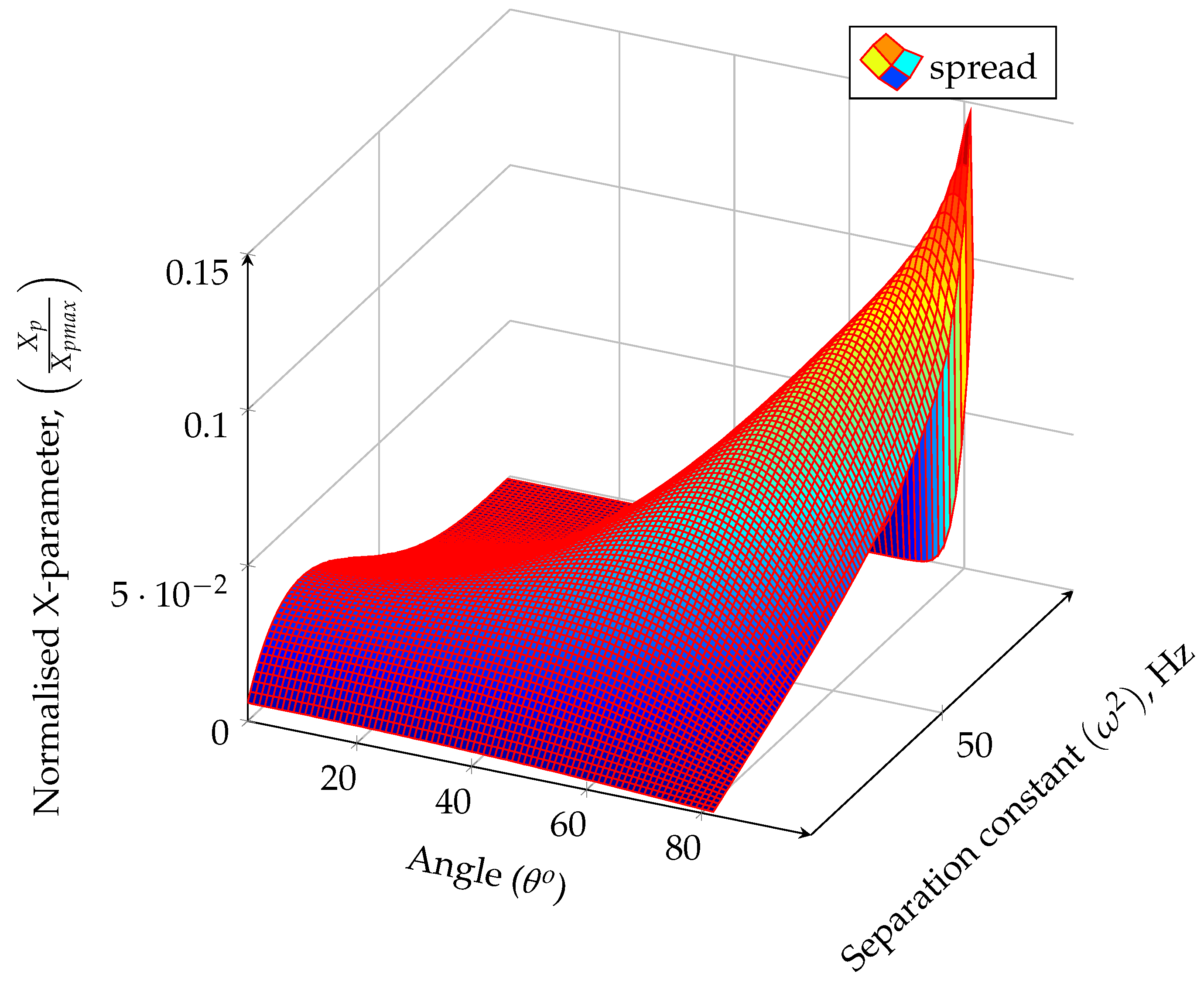
3.3.1. Separation Constant ( ω 2 )

The constant of separation ( ω 2 ) is obtained by rewriting the general advection–dispersion equation (ADE) for the flow of reactive tracers under the influence of linear drift thus:
D 0 β x + d C x x v 0 β x + d C x + D 0 λ y C y y v 0 λ y C y R κ C = R C t ,
where the linear drift ratio is written as d = v d v 0 . The linear drift ratio, d, is coordinate-independent; therefore, its magnitude can be applied equally to the y-axis or, in the case of a 3D system, the z-axis.
Substituting Equation (75) into Equation (87), dividing through by X ( x ) Y ( y , t ) and rearranging (see Appendix C ) gives:
D 0 β x + d X v 0 β x + d X + ω 2 X ( x ) = 0 ,
D 0 λ y Y v 0 λ y Y ( R s + R κ + ω 2 ) Y ( y , s ) = 0 ,
where the component Equation (88) is time-independent, while Equation (89) is time-dependent and expressed in Laplace space with Laplace parameter s. Considering the following transformation parameters:
β = r w cos 2 θ ,
λ = v y r w sin 2 θ ,
x w = r w cos θ ,
y w = r w sin θ ,
Equations (88) and (89) can be rewritten as:
D 0 cos θ + d X v 0 cos θ + d X + ω 2 X ( x w ) = 0 ,
L 1 D 0 ( v y sin θ ) Y v 0 ( v y sin θ ) Y ( R s + R κ + ω 2 ) Y ( y w , s ) = 0 .
Equation (94) is time-independent, while Equation (95) is time-dependent and expressed in Laplace space with Laplace parameter s.

3.3.2. Boundary and Initial Conditions

Equation (87) is governed by the following boundary conditions:
C ( x , y , t = 0 ) = C i ( x , y ) for x = y = R
C ( x = ± , y , t ) = 0 for y = R , t > 0
C ( x , y = ± , t ) = 0 for x = R , t > 0
C ( x w , y w , t ) = C 0 for t > 0
where, the transformation from the polar (radial) coordinate to Cartesian coordinate is given as x w = r w cos θ and y w = r w sin θ . The concentration C ( x w , y w , t ) of the tracer is known within the wellbore during a tracer test; thus, the solution for t > 0 can be obtained by solving Equation (87) within the porous formation outside the wellbore.
The Y-parameter Y p is in Laplace space and requires a numerical inversion scheme, such as the Gaver–Stehfest algorithm [18,29], Talbot inversion algorithm [30] or Euler inversion [31,32] algorithm. The scripts for these algorithms are open source and are readily available for download from the Mathworks website [33]. Out of the two algorithms attempted for the numerical inverse Laplace operation, Gaver–Stehfest and Euler inversion, only the Euler inversion algorithm produced a stable result (see also Avdis and Whitt [34]). Hence, Euler’s Inversion Algorithm was used for the numerical inverse Laplace operation in the numerical code developed for this work.
Flow convection depends on the velocity of the system and is modelled by considering a heterogeneous system. Anisotropic porosity distribution was generated using the random probability density function (PDF) allowing for non-uniform velocity distribution to be computed. Typical porosity distribution is shown in Figure 2 with a mean value of 0.25 and standard deviation of 0.64 . The corresponding computed velocity distribution is shown in Figure 3.

4. Analysis of Results

In this work, the effect of linear drift on the tracer propagation profile in a typical formation of thickness h = 9 m and injection well of radius r w = 0.127 m was investigated. Injected particles are considered to be components of surfactants or polymers used in EOR processes, but in this case, the chemical reaction was neglected. The injection rate was fixed at 1.4 × 10 3 m 3 /s and dispersion coefficient D 0 = 1.4 × 10 3 m 2 /s was applied. The tracer concentration distribution ratio C i was monitored under three continuous injection periods of ten (10) days, fifty (50) days and seventy (70) days respectively.
The developed solution was first tested by evaluating the error limit associated with the separation of variable parameter ( ω 2 ) for different angle θ . Simulation runs involved one hundred (100) values of ω 2 as defined by Equation (81)—ranging from 0.01 × ω 1 2 corresponding to a value of ω 2 = 2.33 × 10 8 to ω 100 2 corresponding to a value of ω 2 = 2.59 × 10 6 —with an incremental value of 0.01 × ω 100 2 . The minimum error corresponds to the value of separation variable ω 2 = 2.33 × 10 8 , as indicated by X p , Y p , t , X Y p , t plots (Figure 4, Figure 5 and Figure 6). The combined solution X Y p , t indicated that there exist points of singularity at 0 ° , 180 ° and 360 ° when taking the inverse of the coordinate point y .
A typical result of the concentration distribution as a function of angle θ obtained from the solution of Equation (75) is shown in Figure 6 for five 5 selected ranges of values of ω 2 . The concentration profile basically grows with increasing values of ω 2 between ω 2 = 2.33 × 10 8 and ω 2 = 1.06 × 10 6 and between θ = 150 ° and θ = 300 ° , after which the impact of drift sets in. With the onset of drift, the concentration profile shortens but with a much wider coverage for ω 2 = 1.58 × 10 6 . The region covered by ω 2 = 2.10 × 10 6 can be seen to have drifted to θ = 240 ° to 300 ° .
In order to further examine the impact of the drift parameter on separation constant ω 2 , X p and angle θ ° , a full simulation run at different time intervals of t = 10 d, t = 30 d, 50 d and 70 d was carried out and results presented in Figure 7, Figure 8, Figure 9 and Figure 10. The magnitude of error due to ω 2 generally reduces with increasing computational time. In Figure 10, the influence of drift is more pronounced. A typical concentration distribution within the porous media with linear drift after 10 days is shown in Figure 11.

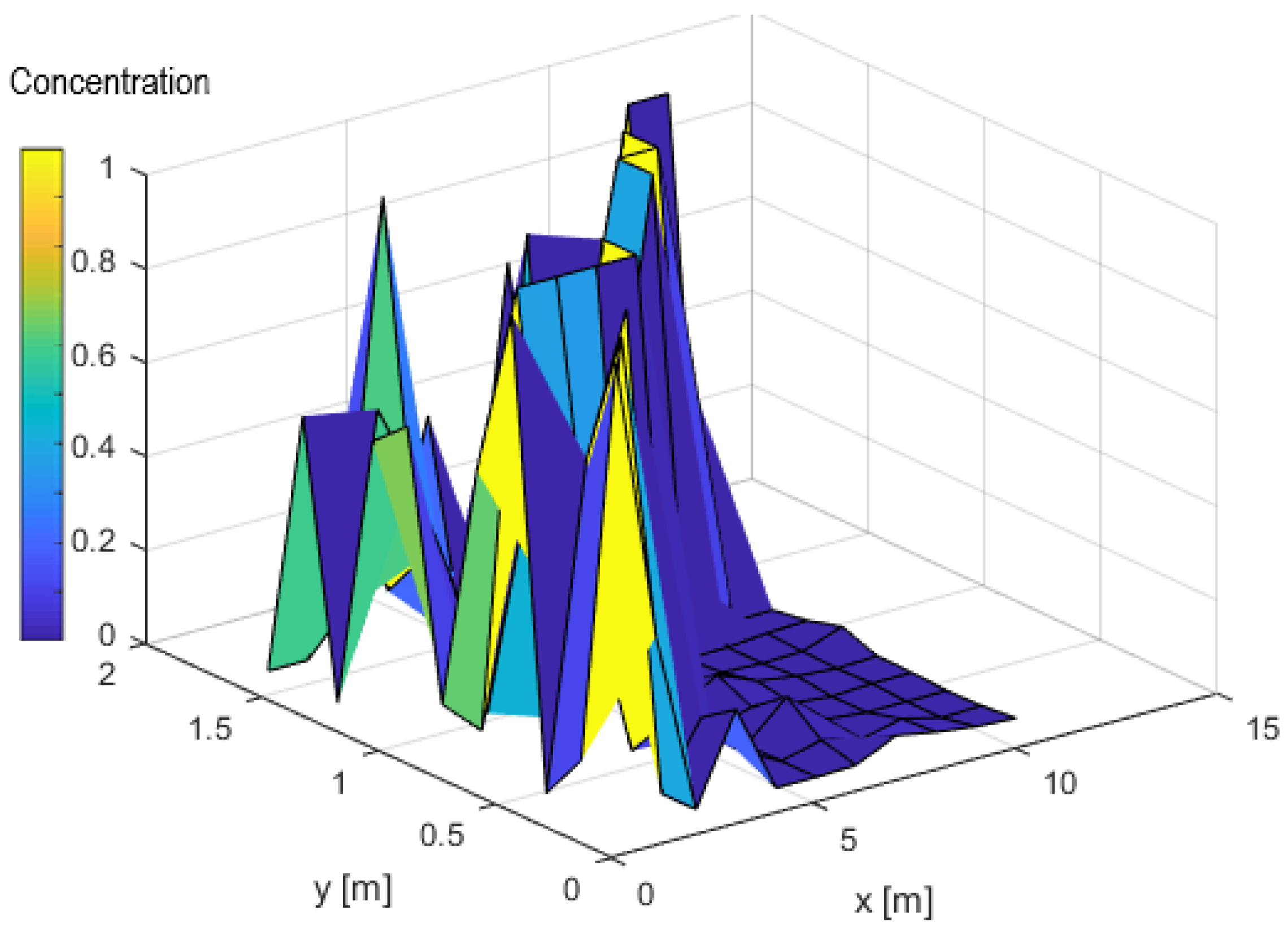
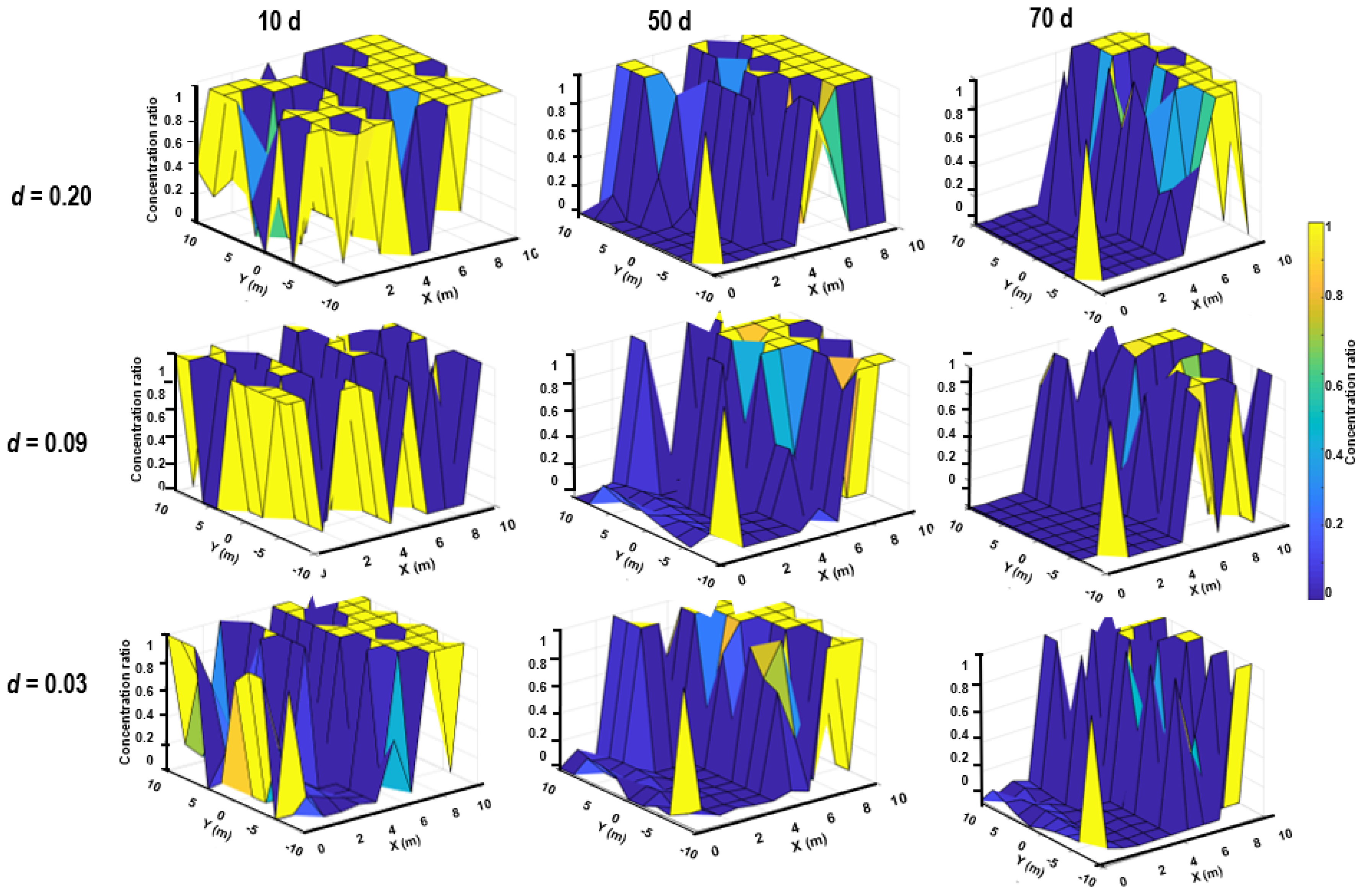
Linear Drift Effect and Concentration Distribution Profile

In a single-well tracer or surfactant injection systems, a primary tracer bank is first injected into a formation containing oil at residual saturation. The bank is then followed by a bank of tracer-free water. The well is then shut in for a period of time, after which the well is produced and the concentration profiles monitored. Where there is fluid migration in the formation due to the movement of an underlying basal water displacing the injected tracer banks during shut-in, the production profile may be distorted and fluid pathway rerouted. In this situation, the effect of linear drift on fluid flow behaviour will have to be investigated.
Generally, in isotropic and homogeneous systems, where there is no linear drift or natural convection, the tracer propagation profile is expected to follow a cyclic pattern. The concentration distribution will be equal at an equidistant radial position from the injection well. In this work, a system with variable porosity distribution was modelled and the corresponding non-uniform velocity profile used in the computation of the drift ratio. In this case, the tracer propagation profile is expected to follow a natural pattern determined by the interplay of the forces associated with the system variables, such as the tracer injection rate.
In order to investigate the effect of the drift intensity on the tracer concentration profile, three (3) values of drift ratio d = 0.03 , 0.09 and 0.2 were evaluated for time duration t = 10 d, 50 d and 70 d. In the presence of linear drift in a heterogeneous system, however, there exists an unequal distribution of tracers along the principal x-axis and varies in a non-uniform manner along the positive and negative radial distance. Where the angle θ increases in the + v e and v e y-axis, the system convection will lead to an increase or decrease in the tracer concentration distribution depending on the degree of system heterogeneity. It is important to note that an increase in the tracer concentration distribution will be observed in a homogeneous system.
The results of the tracer tests for different drift ratios at different time intervals are shown in Figure 12. At a fixed drift ratio (e.g., d = 0.2 ), the effect of the linear drift on the tracer concentration profile is progressively more pronounced at later times; with the lowest tracer concentration ratio at later time indicating a high drift effect. Similarly, at any particular point in time (e.g., at time t = 70 d), linear drift has a greater effect at a higher drift ratio (e.g., d = 0.2 ).

5. Conclusions

The study of the transport of tracers with linear drift is an important aspect of porous media characterisation. Despite the extensive research in this field, particularly in solving the ADE both analytically and numerically, there is yet to be a consideration for the closed-form solution of the ADE in systems where the effect of linear drift may predominate and an exact analytical solution has not been reported in the literature. The following conclusions can be drawn from this work:
  • A new closed-form analytical solution to the radial transport of tracers in porous media under the influence of linear drift and radial convection was developed. The radial transport equation was cast in the form of the Whittaker equation after adopting variable transformation and an exact solution for the tracer concentration derived therefrom.
  • The weak-form solution was developed by splitting the transformed equation, adopting a common separation constant and invoking inverse Laplace transformation using the Euler inversion algorithm.
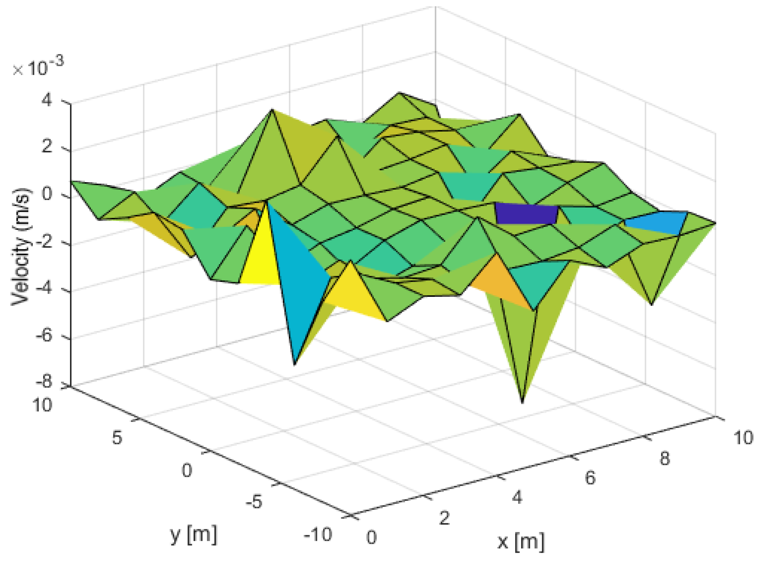
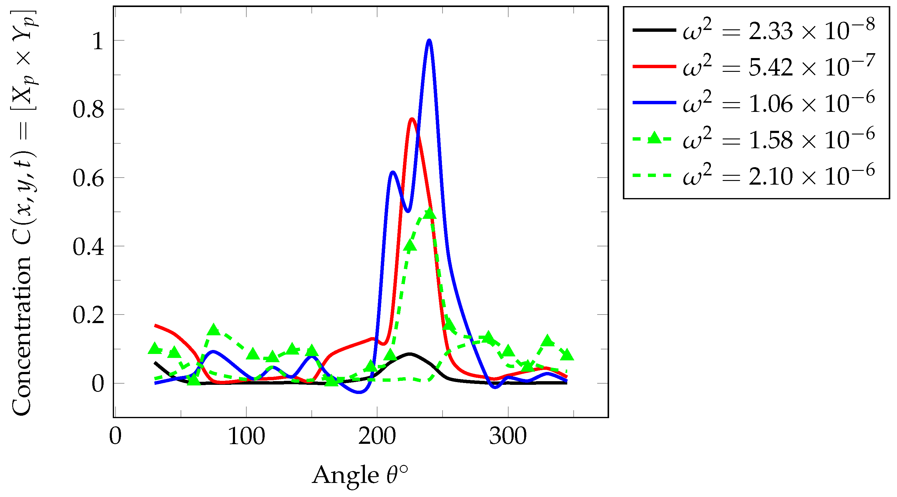
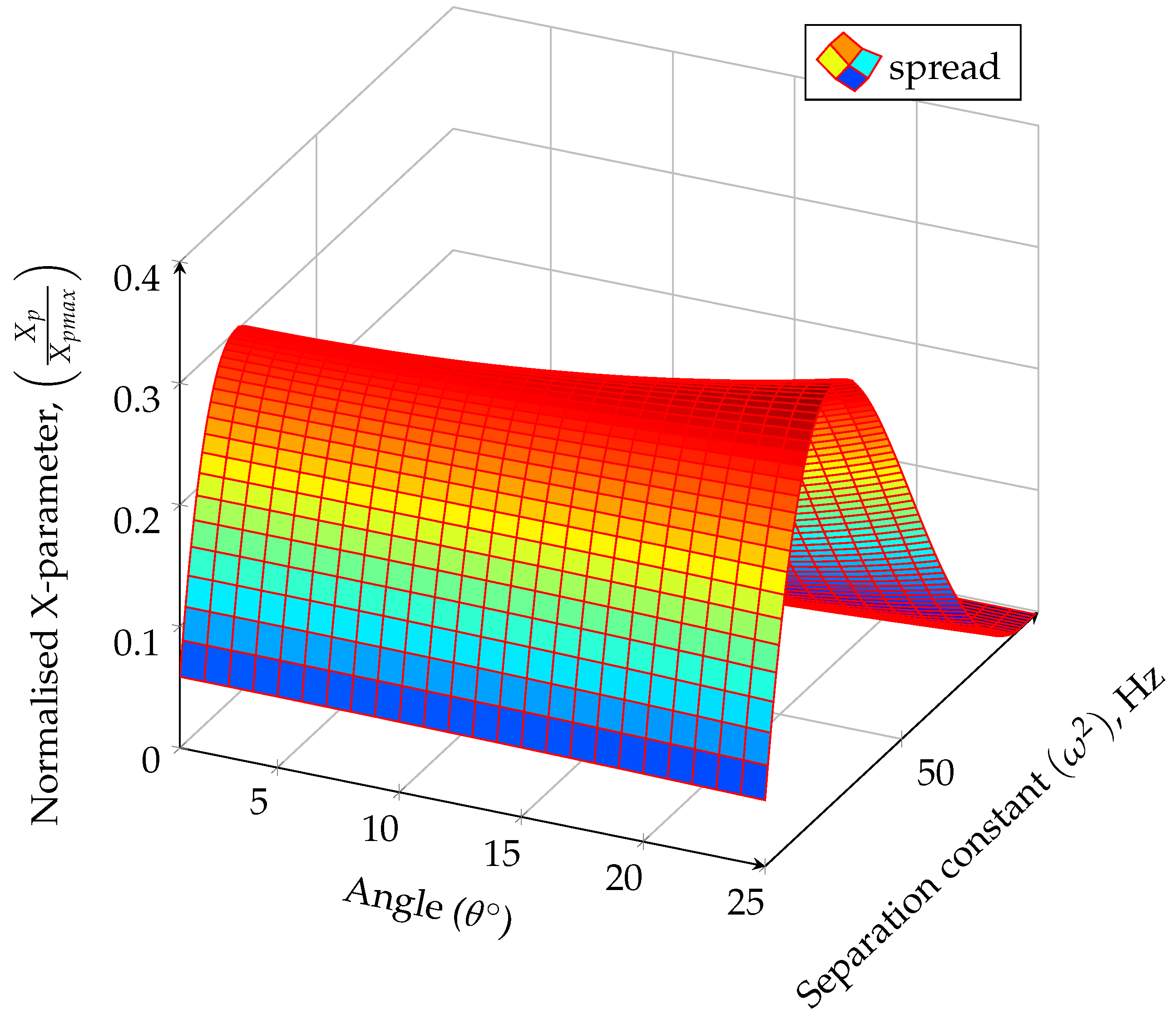
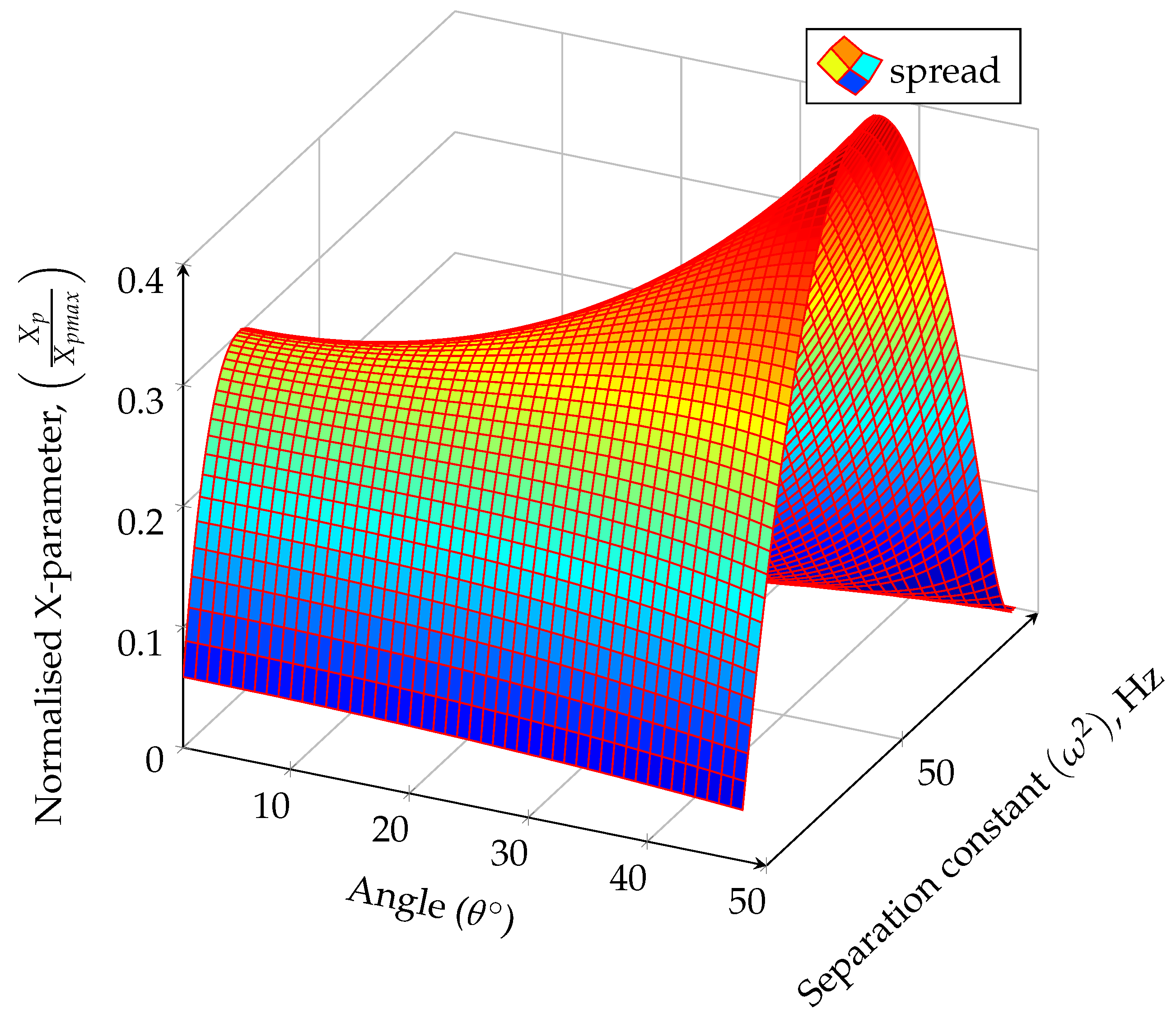
  • Variable transformation from a radial to a Cartesian coordinate system was used to analyse the concentration distribution profiles in three-dimensional graphical plots.
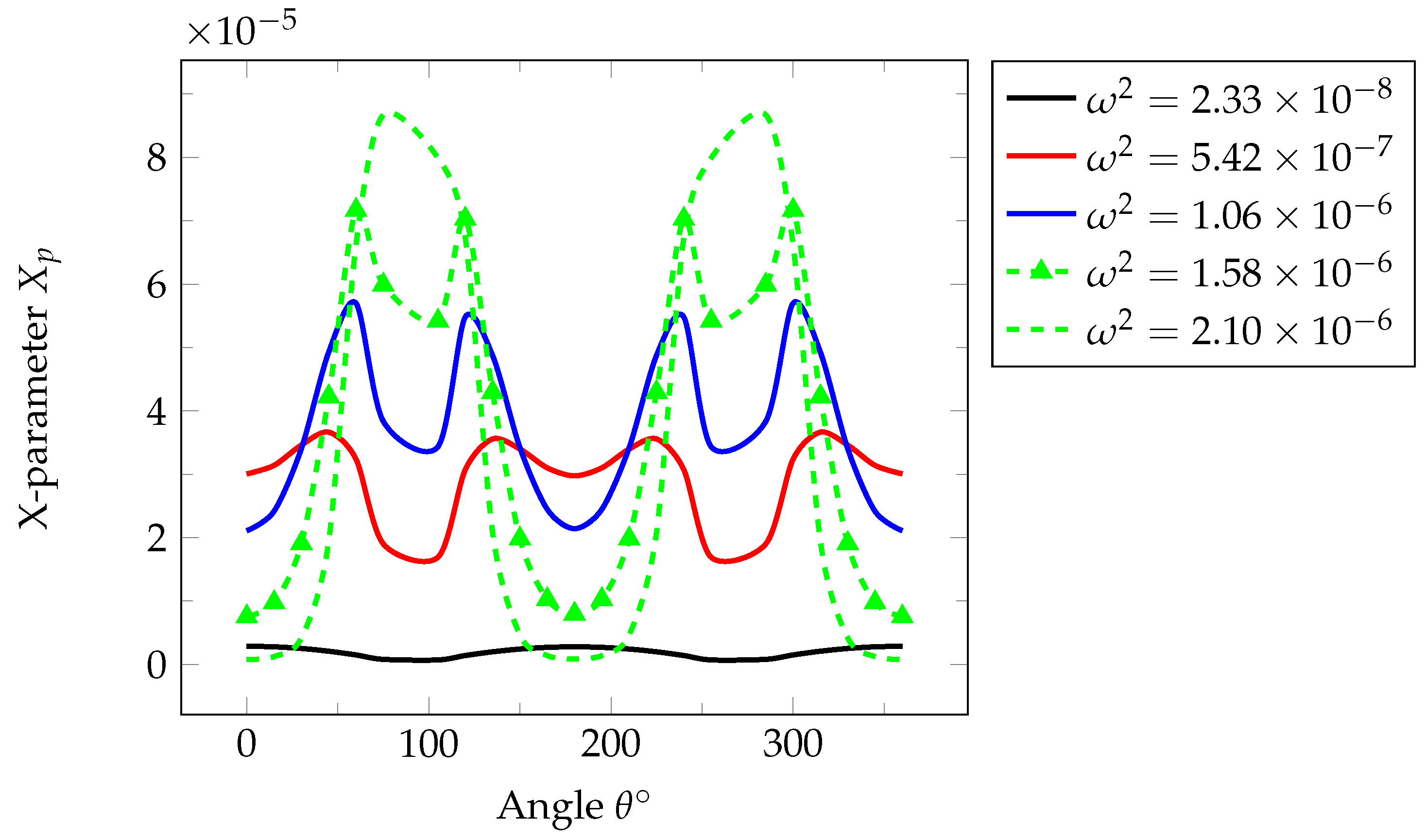
  • The obtained solutions are generally stable and dependent on the precision with which the separation constant ( ω 2 ) can be determined. This is important because the exponential term in the inversion formula may amplify the numerical error. The maximum error quantified by the separation constant is ω 2 = 2.10 × 10 6 .
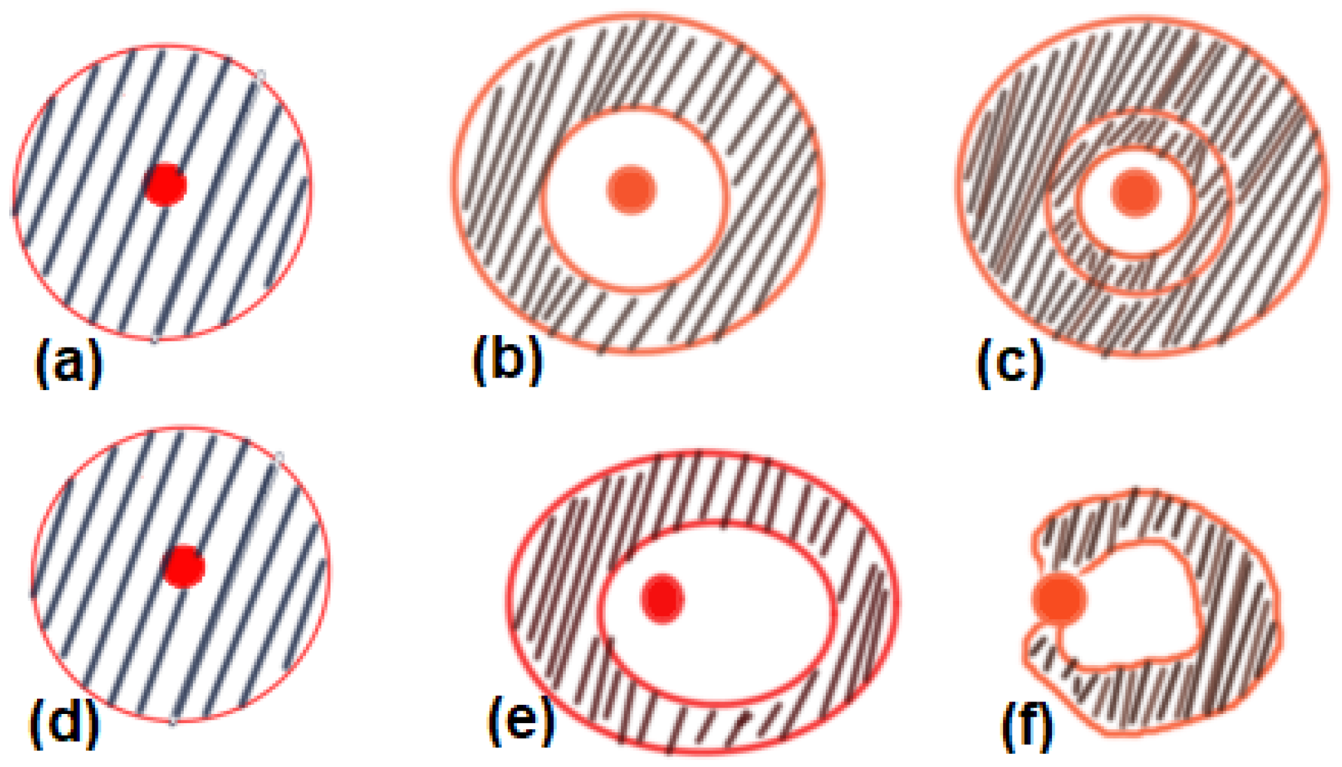
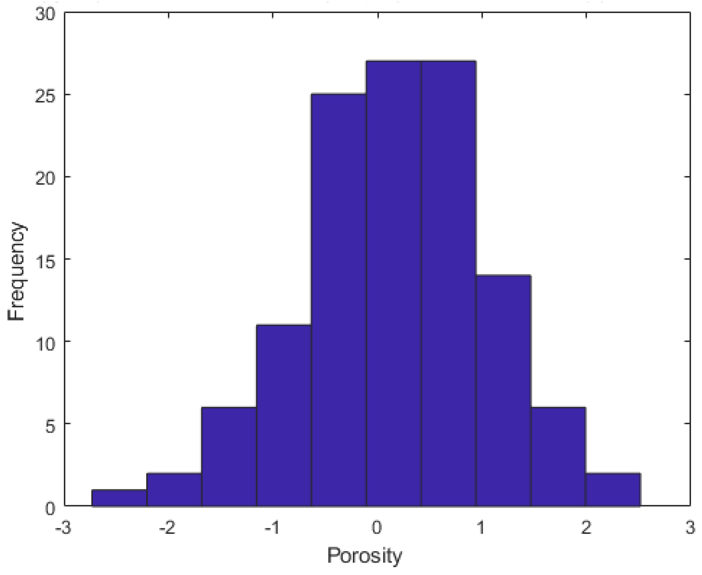
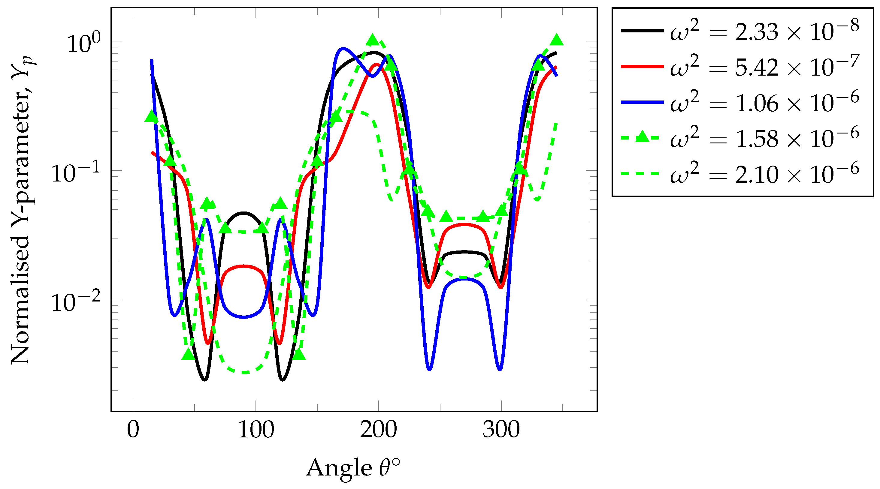
  • The influence of linear drift on the concentration profiles was evaluated in the x-direction for a system with nonhomogeneous porosity distribution and variable velocity profiles.
  • The results of the analyses indicated that the effect of linear drift on the tracer concentration profile is dependent on system heterogeneity and progressively becomes more pronounced at later times.
  • Practical application was demonstrated in a typical EOR process involving the injection of chemicals (e.g., surfactants or polymers), but without a chemical reaction. Another possible application is a single-well chemical tracer injection method for measuring residual oil saturation and fluid flow behaviour and characterisation in porous media.
  • This work can be extended to the analysis of systems involving variation of tracer injection intensity, where spreading may occur in the r- θ or x-y plane. The developed solution can also be extended to systems where moderate-to-high intensity tracer flow with linear drift manifests. In this case, the tangential velocity component of the drift velocity becomes significant and will have to be included in the solution approach.
The new solution to the convective-diffusion equation developed and tested in this work demonstrates the need to study the impact of linear drift on transport of tracers in porous media. This is particularly important, since the arrival times of tracers may be significantly influenced by the drift intensity.

Author Contributions

Conceptualisation, L.T.A. and G.K.F.; Investigation, L.T.A. and G.K.F.; Writing—original draft, L.T.A.; Writing—review and editing, G.K.F. and L.T.A.

Acknowledgments

The authors thank Olakunle Popoola and Ofomana Emmanuel for useful discussions of this topic.

Conflicts of Interest

The authors declare no conflict of interest.

Abbreviations

Γ ( x ) Gamma function
κ , μ Whittaker and Kummer function parameters defined in the text
κ r Chemical reaction constant, (d 1 )
L Laplace operator
ω 2 Absolute value of the separation constant
ϕ Porosity, dimensionless
θ Angle, ( ° )
AConstant of integration
A i ( x ) Airy function of the 1st kind
B i ( x ) Airy function of the 2nd kind
CTracer concentration
DFlow hydrodynamic dispersion (m 2 /s)
dDrift ratio
D m Molecular diffusion constant
D o Shear mixing constant
hFormation thickness, (m)
iUnit vector along the x-axis
jUnit vector along the y-axis
kUnit vector along the z-axis
LLength of dispersion, (m)
QInjection rate, (m 3 /s)
rRadial distance from the well, (m)
r D Dimensionless well-bore radius
r w Well-bore radius, (m)
sLaplace parameter
S m Saturation of the mobile fluid phase
S m p Mobile fluid phase saturation, dimensionless
tTime, (s or d)
uVelocity along the x-axis without linear drift, (m/s)
U ( a , b , z ) Tricomi Kummer U-function with parameters (a,b,z)
u d Linear drift velocity, (m/s)
u o Velocity at the well-bore (m/s)
v y Velocity along the y-axis, (m/s)
W κ , μ ( ξ ) Whittaker function with parameters ( κ , μ )
xx-coordinate variable
yy-coordinate variable
Ddimensionless
ddrift
mmolecular
pphase
rreaction
wwell-bore

Appendix A. Derivation of the Transport Flow Equation with Linear Drift

The flow Equation (1) can be expanded by considering a steady-state condition thus:
1 r D d C d r + r D d C d r + r D d 2 C d r 2 1 r v C + r v C + r v d C d r ϕ ( κ r + s ) C = 0 ,
d 2 C d r 2 + D v D + 1 r d C d r r v + v D r + ϕ ( κ r + s ) D C = 0 ,
where all variables are as defined in the main text. Let:
C = Ψ exp 1 2 D v D + 1 r d r .
Then:
d C d r = d Ψ d r · e 1 2 D v D + 1 r 1 2 D v D + 1 r Ψ e 1 2 D v D + 1 r ,
and:
d 2 C d r 2 = d d r d Ψ d r · e 1 2 D v D + 1 r 1 2 D v D + 1 r Ψ e 1 2 D v D + 1 r = d 2 Ψ d r 2 · e 1 2 D v D + 1 r 1 2 D v D + 1 r d Ψ d r e 1 2 D v D + 1 r 1 2 D v D + 1 r Ψ e 1 2 D v D + 1 r 1 2 D v D + 1 r d Ψ d r e 1 2 D v D + 1 r + 1 4 D v D + 1 r 2 Ψ e 1 2 D v D + 1 r
d 2 C d r 2 = d 2 Ψ d r 2 D v D + 1 r d Ψ d r 1 2 D v D + 1 r 1 4 D v D + 1 r 2 Ψ e 1 2 D v D + 1 r .
Let:
d 2 C d r 2 + D v D + 1 r d C d r = I ,
with the first order differential component d C d r defined by Equation (A4), then:
I = d 2 Ψ d r 2 e 1 2 D v D + 1 r D v D + 1 r d Ψ d r e 1 2 D v D + 1 r 1 2 D v D + 1 r 1 4 D v D + 1 r 2 Ψ e 1 2 D v D + 1 r + D v D + 1 r e 1 2 D v D + 1 r d Ψ d r 1 2 D v D + 1 r Ψ e 1 2 D v D + 1 r .
Applying Equations (A3) and (A8) in (A1) and rearranging yields:
d 2 Ψ d r 2 1 2 D v D + 1 r + 1 4 D v D + 1 r 2 + r v + v D r + ϕ ( κ r + s ) D Ψ = 0 .
Expressing the effective fluid velocity v in dimensionless form:
v = v d + α r ,
D ( r ) = β w r 2 ,
v = α r 2 .
Thus:
D ( r ) v = β w r 2 α ω ¯ + 1 r
= β w r 2 α ( ω ¯ r + 1 ) r
D ( r ) v D ( r ) = β w r 2 r κ r + β w α ( ω ¯ r + 1 ) κ r + β w
= β w r ( κ r + β w ) α ( ω ¯ r + 1 ) κ r + β w .
Let:
I β w r ( κ r + β w )
A r + C κ r + β w ,
then:
( A κ + C ) r + A β w = β w .
Thus, A = 1 and C = κ , so that:
β w r ( κ r + β w ) = κ ( κ r + β w ) 1 r .
Therefore:
D ( r ) v D ( r ) = κ ( κ r + β w ) 1 r α ( ω ¯ r + 1 ) ( κ r + β w ) ,
D ( r ) v D ( r ) + 1 r = κ ( κ r + β w ) α ( ω ¯ r + 1 ) ( κ r + β w ) .
Similarly:
D ( r ) v D ( r ) + 1 r = κ 2 ( κ r + β w ) 2 α ω ¯ ( κ r + β w ) + α κ ( ω ¯ r + 1 ) ( κ r + β w ) 2 = α κ ( ω ¯ r κ 2 ) ( κ r + β w ) 2 α ω ¯ ( κ r + β w ) .
Additionally:
r v = r · α r 2 = α r ,
and:
r v + v = α r + α ω ¯ + 1 r = α r + α ω ¯ r + 1 r = α ω ¯ .
Thus:
r v + v D ( r ) r = α ω ¯ ( κ r + β w ) .
Therefore, Equation (A9) becomes:
d 2 Ψ d r 2 1 2 α κ ( ω ¯ r + 1 ) κ 2 ( κ r + β w ) 2 α ω ¯ ( κ r + β w ) + 1 4 κ α ( ω ¯ r + 1 ) ( κ r + β w ) 2 + α ω ¯ + ϕ ( κ r + s ) r κ r + β w Ψ = 0 ,
or:
d 2 Ψ d r 2 1 2 α κ ( ω ¯ r + 1 ) κ 2 ( κ r + β w ) 2 α ω ¯ 2 ( κ r + β w ) Ψ + 1 4 κ 2 ( κ r + β w ) 2 + α 2 ( ω ¯ r + 1 ) 2 ( κ r + β w ) 2 2 α κ ( ω ¯ r + 1 ) ( κ r + β w ) 2 Ψ + α ω ¯ + ϕ ( κ r + s ) r κ r + β w Ψ = 0 ,
d 2 Ψ d r 2 α κ ( ω ¯ r + 1 ) 2 ( κ r + β w ) 2 κ 2 2 ( κ r + β w ) 2 α ω ¯ 2 ( κ r + β w ) + k 2 4 ( κ r + β w ) 2 Ψ + α 2 ( ω ¯ r + 1 ) 2 4 ( κ r + β w ) 2 α κ ( ω ¯ r + 1 ) 2 ( κ r + β w ) 2 + α ω ¯ κ r + β w + ϕ ( κ r + s ) r κ r + β w Ψ = 0 .
An expression of the form:
d 2 Ψ d r 2 α 2 ω ¯ r + 1 2 κ 2 4 ( κ r + β w ) 2 + α ω ¯ 2 ( κ r + β w ) + ϕ ( κ r + s ) r ( κ r + β w ) Ψ = 0 ,
is therefore obtained for the general convection–diffusion equation in Laplace space. This can be written in dimensionless form as:
d 2 Ψ d r D 2 α 2 ω r D + 1 2 κ 2 4 ( κ r D + β ) 2 + α ω 2 ( κ r D + β w ) + ϕ ( κ r + s ) r D ( κ r D + β ) Ψ = 0 ,
where the variables are redefined as:
D ( r D k ) = D m + v m D o ω + 1 r D ,
= κ + β r D ,
and:
κ = D m + β ω .
Using Equations (23) and (24) in Equation (A29) yields:
κ 2 d 2 Ψ d η 2 α 2 ω 2 4 κ 2 α 2 ω 2 κ ω β κ 1 1 η + 1 4 η 2 α 2 ω β κ 1 2 κ 2 Ψ + α ω 2 η + ϕ ( κ r + s ) κ β ϕ ( κ r + s ) κ η Ψ = 0 .

Appendix B. Analytical Solution—Dimensionless Representation and Inverse Laplace Transform

In dimensionless radial length r D , C ( η ( r ) , s ) can be written as:
C ( η ( r ) , s ) = Ψ e 1 2 κ α κ r D + β + α ω r D κ r D + β d r D
= Ψ e 1 2 κ κ α η + α ω κ ( η β ) η d η
C ( η ( r ) , s ) = Ψ e 1 2 κ α α ω κ η + α ω κ d η
ψ ( ξ , s ) = e ξ 2 ξ 1 2 + μ U ( 1 2 + μ κ , 1 + 2 μ , ξ )
A ( s ) = 2 k 2 α k α ω β 2 k 2 ξ k 2 α k α ω β 2 k 2 μ 1 2 f ( s ) k 2 α k α ω β 2 k 2 ,
but:
B ( s ) = C ξ , s 2 k 2 α k α ω β 2 k 2 ξ k 2 α k α ω β 2 k 2 μ 1 2 f ( s ) k 2 α k α ω β 2 k 2 E x p ξ 2 1 + α ω 2 k 2 f ( s ) U ( 1 2 + μ κ , 1 + 2 μ , ξ )
.
Therefore:
d C ( ξ , s ) d ξ = ( μ + 1 2 ) ξ 1 U 1 2 ( 1 + α ( ω β k ) 2 k f ( s ) ) U ( 1 2 + μ κ ) d U ( 1 2 + μ κ , 1 + 2 μ , ξ ) d ξ C ( ξ , s ) A ( s ) e ξ 2 ( 1 + α ( ω β k 1 ) k 2 f ( s ) ) 2 k 2 α k α ω β 2 k 2 ξ k 2 α k α ω β 2 k 2 μ 1 2 f ( s ) k 2 α k α ω β 2 k 2 E x p ξ 2 1 + α ω 2 k 2 f ( s ) U ( 1 2 + μ κ , 1 + 2 μ , ξ )
d C ( ξ , s ) d ξ = ( μ + 1 2 ) ξ 1 U 1 2 ( 1 + α ( ω β k ) 2 k f ( s ) ) U ( 1 2 + μ κ ) d U ( 1 2 + μ κ , 1 + 2 μ , ξ ) d ξ C ( ξ , s ) U ( 1 2 + μ κ , 1 + 2 μ , ξ )
d C ( ξ , s ) d ξ = 1 ξ ( μ + 1 2 ) 1 2 ( 1 + α ( ω β k ) 2 k f ( s ) ) ( 1 2 + μ K ) d U ( 1 2 + μ κ , 1 + 2 μ , ξ ) d U ( 1 2 + μ κ , 1 + 2 μ , ξ ) C ( ξ , s ) .
Therefore:
d C ( ξ , s ) d r D = 2 k f ( s ) 1 ξ ( μ + 1 2 ) 1 2 ( 1 + α ( ω β k ) 2 k f ( s ) ) ( 1 2 + μ κ ) d U ( 1 2 + μ κ , 1 + 2 μ , ξ ) d U ( 1 2 + μ κ , 1 + 2 μ , ξ ) C ( ξ , s )
but:
U ( 1 2 + μ κ , 1 + 2 μ , ξ ) U ( 1 2 + μ κ , 1 + 2 μ , ξ ) = 1 ξ = 1 2 η f ( s )
d C ( ξ , s ) d η = 2 k f ( s ) 1 ξ ( μ + 1 2 ) 1 2 ( 1 + α ( ω β k ) 2 k f ( s ) ) ( 1 2 + μ κ ) 1 ξ C ( ξ , s )
1 f ( s ) d C ( ξ , s ) d r D = 2 κ K ξ 1 2 ( 1 + α ( ω β κ ) 2 κ f ( s ) ) C ( ξ , s ) = κ K η f ( s ) 1 α ( ω β κ ) 2 κ f ( s ) C ( ξ , s ) .
However:
K = ω α 4 κ 2 α κ ω β 2 κ 1 1 f ( s ) β 2 f ( s )
1 f ( s ) d C ( ξ , s ) d η = ω α 2 κ α κ ω β 2 κ 1 1 f ( s ) k β 2 f ( s ) η f ( s ) k α ( ω β κ ) 2 f ( s ) C ( ξ , s )
1 f ( s ) d C ( ξ , s ) d η = ω α 2 k α k ω β 2 k 1 1 η f ( s ) 2 k β 2 η k α ( ω β k ) 2 f ( s ) C ( ξ , s )
1 f ( s ) d C ( ξ , s ) d η = k ( 1 + β 2 η ) + α ( ω β k ) 2 f ( s ) ω α 2 k α k ω β 2 k 1 1 η f ( s ) 2 C ( ξ , s )
1 f ( s ) d C ( ξ , s ) d η = k ( 1 + β 2 η ) + 1 2 α ω β k f ( s ) ω α 2 η k α k ω β 2 k 1 1 f ( s ) 2 C ( ξ , s ) .
Rearranging:
( 1 + β 2 η ) C ( ξ , s ) = 1 k f ( s ) d C ( ξ , s ) d η 1 2 α ω β k k f ( s ) ω α 2 η α k ω β 2 k 1 1 k 2 f ( s ) 2 C ( ξ , s )
k f ( s ) = α 2 ω 2 4 k 2 + φ ( k r + s ) k = φ k α 2 ω 2 4 φ k + k r + s .
The Inverse Laplace Transform of f ( s ) 1 is:
L 1 1 φ k α 2 ω 2 4 φ k + k r + s = e α 2 ω 2 4 φ k + k r t φ κ π t .
Similarly, the inverse Laplace transform of f ( s ) 2 is:
L 1 1 φ k α 2 ω 2 4 φ k + k r + s 2 = e α 2 ω 2 4 φ k + k r t φ κ .
Evaluating the inverse Laplace transform of the general solution:
( 1 + β 2 η ) C ( ξ , t ) = κ φ 0 t d C ( ξ , τ ) d η e α 2 ω 2 4 φ κ + κ r ( t τ ) π ( t τ ) d τ κ φ α ω β κ 0 t C ( ξ , t ) e α 2 ω 2 4 φ κ + κ r ( t τ ) π ( t τ ) d τ + α ω κ 2 η φ α κ ω β 2 κ 1 1 0 t C ( ξ , τ ) e α 2 ω 2 4 φ κ + κ r ( t τ ) d τ
κ = D m + β ω = D m 1 + β ω D m ,
f ( s ) = 1 κ α 2 ω 2 4 κ 2 + φ ( κ r + s ) κ = 1 D m + β ω α 2 ω 2 4 ( D m + β ω ) 2 + φ ( κ r + s ) D m + β ω .
Equations (39) and (40) respectively become:
μ = α D m 2 ( 1 + D 0 υ d D m ) 2 ,
and:
K = ( 1 + D 0 υ d D m ) 2 α D 0 υ d D 0 υ d D m + 2 ϕ 1 + D 0 υ d D m ( k r + s ) 4 1 + D 0 υ d D m 2 1 + 4 ϕ D m D 0 υ d 2 1 + D 0 υ d D m ( k r + s ) ,
here:
ϕ = ϕ D 0 2 D m .

Appendix C. Weak-Form Solution—Separation Constant and Extended Confluent Hypergeometric Functions

Rewriting Equation (88) as:
β + x d X v 0 D 0 β + x d X μ D 0 x X = 0 ,
and expressing in terms of the variable x defined in relation to the drift ratio d as x = x 1 β d and also defining the 1st-order and 2nd-order differentials in terms of x 1 :
β + x d X v 0 D 0 β + x d X μ D 0 x X = 0 ,
x 1 X v 0 D 0 d x 1 X μ d 3 D 0 x 1 μ β d 3 D 0 X = 0 .
Similarly, defining x 1 = D 0 d v 0 x 2 in Equation (A64) and the 1st-order and 2nd-order differential in relation to x 2 :
v 0 D 0 d x 2 X v 0 D 0 d x 2 X μ v 0 d 2 x 2 μ β v 0 d 2 X = 0 ,
multiplying Equation (A65) by D 0 d v 0 and expressing in terms of x 2 :
x 2 X x 2 X μ D 0 v 0 d 2 x 2 μ D 0 v 0 2 d X = 0 .
Equation (A66) is comparable to the extended confluent hypergeometric equation of degree N [35]:
x X + ( γ x ) X α + n = 1 N α n x n X = 0 ,
with one of its solutions being the extended confluent hypergeometric function:
X 1 ( x ) = 1 F 1 N ( α ; γ ; A a , , A N ; x ) ,
where the lower-case subscripts are the same as for the original confluent hypergeometric function:
1 F 1 N ( α ; γ ; x ) = 1 F 1 0 ( α ; γ ; x )
= 1 F 1 N ( α ; γ ; 0 , , 0 ; x ) ,
and the upper case subscript, N = 0 in this case, and an arbitrary positive integer in general [35].
Equation (A66) is comparable to the extended confluent hypergeometric equation of degree 1 (Equation (A67)) thus:
x X + ( γ x ) X ( α + α 1 x ) X = 0 ,
where:
n = 1
γ = 0
α = μ β v 0 d 2
α 1 = μ D 0 v 0 2 d .
The extended confluent hypergeometric function of degree one can be obtained by introducing:
σ ± = 1 / 2 ± 1 / 4 + α 1
= 1 4 ω 2 D 0 v 0 2 d ,
and the first kind leads to the integral representation:
Re ( γ ) > Re ( α ) > 0 : F ( α ; γ ; x ) = D + 0 1 z α 1 ( z 1 ) γ α 1 e x z d z ,
and the second kind leads to the integral representation:
Re ( γ ) > 0 , Re ( α ) > 0 : G ( α ; γ ; x ) = D e i π γ 0 z α 1 ( z + 1 ) γ α 1 e z x d z ,
where the constants D ± chosen are:
D = e i r γ i Γ ( α ) ,
and D + takes the value unity at the origin. The solution of Equation (A71) is in the form of extended confluent hypergeometric function of degree one and 2nd kind:
Re ( x 2 ) > 0 , Re ( α ) > 0 : X ( x 2 ) = 1 G 1 1 ( α ; γ ; α 1 ; x 2 ) = e 1 2 1 σ 1 x 2 Γ ( α ) 0 z α σ 1 ( z + 1 ) α σ + 1 e σ z x 2 d z
x 1 = β + x d
x 2 = v 0 D 0 d x 1
μ = ω 2
ω 2 = | μ |
Defining the Tricomi–Kummer function [36,37]:
U ( a , b , x ) = 1 Γ ( α ) 0 z α 1 ( z + 1 ) ( α + 1 b ) e z x d z ,
and rearranging:
Γ ( α ) U ( a , b , x ) = 0 z α 1 ( z + 1 ) ( α + 1 b ) e z x d z .
For the Y-component, substituting Equation (A83) in Equation (89) and multiplying by y λ D 0 gives:
Y v 0 D 0 Y R s + R κ + ω 2 D 0 λ y Y ( y , s ) = 0 .
The following variables are hereby defined:
Y = ψ e v 0 y 2 D 0
Y = ψ e v 0 y 2 D 0 + v 0 2 D 0 ψ e v 0 y 2 D 0
Y = ψ e v 0 y 2 D 0 + v 0 D 0 ψ e v 0 y 2 D 0 + 1 4 v 0 D 0 2 ψ e v 0 y 2 D 0 ,
and transform Equation (A87) thus:
ψ D 0 λ R s + R κ + ω 2 2 y 1 ψ = 0 ,
which is a general form of the Airy equation.

References

  1. Baldwin, D.E. Prediction of Tracer Performance in a Five-Spot Pattern. J. Pet. Technol. 1966, 18, 513–517. [Google Scholar] [CrossRef]
  2. Rubin, J.; James, R.V. Dispersion affected transport of reacting solutes in saturated porous media: Galerkin Method applied to equilibrium-controlled exchange in unidirectional steady water flow. Water Resour. Res. 1973, 9, 1332–1356. [Google Scholar] [CrossRef]
  3. Moreno, L.; Neretnieks, I.; Klockars, C.E. Evaluation of Some Tracer Test in the Granitic Rock at FinnsjöRn; SKBF/KBS Tech; Technical Report 83-38; Nuclear Fuel Safety Project; SKB: Stockholm, Sweden, 1983. [Google Scholar]
  4. Herbert, A.W.; Hodgkinson, D.P.; Lever, D.A.; Rae, J.; Robinson, P.C. Mathematical modelling of radionuclide migration in groundwater. Q. J. Eng. Geol. 1986, 19, 109–120. [Google Scholar] [CrossRef]
  5. Mabuza, S.; Čanić, S.; Muha, B. Modeling and analysis of reactive solute transport in deformable channels with wall adsorption-desorption. Math. Methods Appl. Sci. 2016, 39, 1780–1802. [Google Scholar] [CrossRef]
  6. Vetter, O.J.; Zinnow, K.P. Evaluation of Well-to-Well Tracers for Geothermal Reservoirs; Lawrence Berkeley National Laboratory: Berkeley, CA, USA, 1981; Volume 14.
  7. Tomich, J.F.; Dalton, R.L.J.; Deans, H.A.; Shallenberger, L.K. Single-Well Tracer Method To Measure Residual Oil Saturation. J. Pet. Technol. 1973, 25, 211–218. [Google Scholar] [CrossRef]
  8. Bear, J. Dynamics of Fluids in Porous Media; Dover Civil and Mechanical Engineering; Dover Publications: Mineola, NY, USA, 2013. [Google Scholar]
  9. Zhou, R.; Zhan, H. Reactive solute transport in an asymmetrical fracture-rock matrix system. Adv. Water Resour. 2018, 112, 224–234. [Google Scholar] [CrossRef]
  10. Landa-Marbán, D.; Radu, F.A.; Nordbotten, J.M. Modeling and Simulation of Microbial Enhanced Oil Recovery Including Interfacial Area. Transp. Porous Media 2017, 120, 395–413. [Google Scholar] [CrossRef] [Green Version]
  11. Noetinger, B.; Roubinet, D.; Russian, A.; Borgne, T.L.; Delay, F.; Dentz, M.; de Dreuzy, J.; Gouze, P. Random Walk Methods for Modeling Hydrodynamic Transport in Porous and Fractured Media from Pore to Reservoir Scale. Transp. Porous Media 2016, 115, 345–385. [Google Scholar] [CrossRef] [Green Version]
  12. Zlotnik, V.A.; Logan, J.D. Boundary conditions for convergent radial tracer tests and effect of well bore mixing volume. Water Resour. Res. 1996, 32, 2323–2328. [Google Scholar] [CrossRef]
  13. Carslaw, H.S.; Jaeger, J.C. Conduction of Heat in Solids; Clarendon Press: Oxford, UK, 1959. [Google Scholar]
  14. Falade, G.K.; Brigham, W.E. Analysis of Radial Transport of Reactive Tracer in Porous Media. SPE Reserv. Eng. 1989, 4, 85–90. [Google Scholar] [CrossRef]
  15. Attinger, S.; Abdulle, A. Effective velocity for transport in heterogeneous compressible flows with mean drift. Phys. Fluids 2008, 20, 016102. [Google Scholar] [CrossRef] [Green Version]
  16. Vergassola, M.; Avellaneda, M. Scalar transport in compressible flow. Phys. D Nonlinear Phenom. 1997, 106, 148–166. [Google Scholar] [CrossRef] [Green Version]
  17. Moench, A.F.; Ogata, A. A numerical inversion of the Laplace transform solution to radial dispersion in a porous medium. Water Resour. Res. 1981, 17, 250–252. [Google Scholar] [CrossRef]
  18. Stehfest, H. Algorithm 368: Numerical inversion of Laplace transforms. Assoc. Comput. Mach. J. 1970, 13, 47–49. [Google Scholar]
  19. Abramowitz, M.; Stegun, I.A. Handbook of Mathematical Functions, Appl. Math. Ser. 55; National Bureau of Standards: Gaithersburg, MD, USA, 1964; p. 1046.
  20. Mashayekhizadeh, V.; Dejam, M.; Ghazanfari, M.H. The Application of Numerical Laplace Inversion Methods for Type Curve Development in Well Testing: A Comparative Study. Pet. Sci. Technol. 2011, 29, 695–707. [Google Scholar] [CrossRef]
  21. De-Hoog, F.R.; Knight, D.H.; Stokes, A.N. An Improved Method for Numerical Inversion of Laplace Transforms. SIAM J. Sci. Stat. Comput. 1982, 3, 357–366. [Google Scholar] [CrossRef]
  22. Dubner, H.; Abate, J. Numerical Inversion of Laplace Transforms by Relating Them to the Finite Fourier Cosine Transform. Assoc. Comput. Mach. J. 1968, 15, 115–123. [Google Scholar] [CrossRef]
  23. Zakian, V. Numerical inversion of Laplace transform. Electron. Lett. 1969, 5, 120–121. [Google Scholar] [CrossRef]
  24. Schapery, R.A. Approximate methods of transform inversion for viscoelastic stress analysis. In Proceedings of the 4th U.S. National Congress on Applied Mechanics, Berkeley, CA, USA, 18–21 June 1962; pp. 1075–1085. [Google Scholar]
  25. Brzeziński, D.W.; Ostalczyk, P. Numerical calculations accuracy comparison of the Inverse Laplace Transform algorithms for solutions of fractional order differential equations. Nonlinear Dyn. 2016, 84, 65–77. [Google Scholar] [CrossRef]
  26. Fick, A. Ueber Diffusion. Ann. Phys. 1855, 94, 59–86. (In German) [Google Scholar] [CrossRef]
  27. Skellam, J. Random Dispersal in Theoretical Populations. Biometrika 1951, 38, 196–218. [Google Scholar] [CrossRef] [PubMed]
  28. Whittaker, E.T. An expression of certain known functions as generalized hypergeometric functions. Bull. Am. Math. Soc. 1903, 10, 125–134. [Google Scholar] [CrossRef]
  29. Gaver, D.P. Observing stochastic processes and approximate transform inversion. Oper. Res. 1966, 14, 444–459. [Google Scholar] [CrossRef]
  30. Talbot, A. The accurate numerical inversion of Laplace transforms. IMA J. Appl. Math. 1979, 23, 97–120. [Google Scholar] [CrossRef]
  31. Abate, J.; Whitt., W. The Fourier-series method for inverting transforms of probability distributions. Queueing Syst. 1992, 10, 5–88. [Google Scholar] [CrossRef]
  32. Abate, J.; Whitt., W. Numerical inversion of Laplace transforms of probability distributions. Oper. Res. Soc. Am. J. Comput. 1995, 7, 36–43. [Google Scholar] [CrossRef]
  33. McClure, T. Numerical Inverse Laplace Transform. 2018. Available online: https://uk.mathworks.com/matlabcentral/fileexchange/39035-numerical-inverse-laplace-transform (accessed on 16 August 2017).
  34. Avdis, E.; Whitt, W. Power Algorithms for Inverting Laplace Transforms. INFORMS J. Comput. 2007, 19, 341–355. [Google Scholar] [CrossRef] [Green Version]
  35. Campos, L. On some solutions of the extended confluent hypergeometric differential equation. J. Comput. Appl. Math. 2001, 137, 177–200. [Google Scholar] [CrossRef]
  36. Spanier, J.; Oldham, K.B. An Atlas of Functions; Taylor & Francis/Hemisphere: Bristol, PA, USA, 1987. [Google Scholar]
  37. Slater, L.J. The Second Form of Solutions of Kummer’s Equations; Confluent Hypergeometric Functions; Cambridge University Press: Cambridge, UK, 1960. [Google Scholar]
Figure 1. Schematic representation of chemical tracer method in a single well test involving injection of tracer (ac) without drift and (df) with drift.
Energies 12 00029 g001
Figure 2. Porosity distribution profile generated using random probability density function. [ ] denotes that the variable has no unit.
Energies 12 00029 g002
Figure 3. Typical spatial heterogeneous porous system velocity distribution (m/s) used in the numerical computation.
Energies 12 00029 g003
Figure 4. X-parameter ( X p ) as a function of angle ( θ ° ) at a fixed time t = 10 d and varying separation constant ( ω 2 ).
Energies 12 00029 g004
Figure 5. Y-parameter ( Y p ) as a function of angle ( θ ° ) at a fixed time t = 10 d and varying separation constant ( ω 2 ).
Energies 12 00029 g005
Figure 6. Concentration profile versus angle ( θ ° ) and varying separation constant ( ω 2 ).
Energies 12 00029 g006
Figure 7. 3D plot of X-parameter ( X p ) as a function of the separation constant ( ω 2 ) and angle ( θ ° ) at time t = 10 d.
Energies 12 00029 g007
Figure 8. 3D plot of X-parameter ( X p ) as a function of the separation constant ( ω 2 ) and angle ( θ ° ) at time t = 30 d.
Energies 12 00029 g008
Figure 9. 3D plot of X-parameter ( X p ) as a function of the separation constant ( ω 2 ) and angle ( θ ° ) at time t = 50 d.
Energies 12 00029 g009
Figure 10. 3D plot of X-parameter ( X p ) as a function of the separation constant ( ω 2 ) and angle ( θ ° ) at time t = 70 d.
Energies 12 00029 g010
Figure 11. Typical concentration distribution within the porous media with low linear drift ratio d = 0.006 after 10 days.
Energies 12 00029 g011
Figure 12. Concentration distribution within the porous media with linear drift ratio d = 0.03 , 0.09 and 0.2 and time interval t = 10 d, 50 d and 70 d.
Energies 12 00029 g012

