How Adding a Battery to a Grid-Connected Photovoltaic System Can Increase its Economic Performance: A Comparison of Different Scenarios


Abstract
1. Introduction
2. Methodology
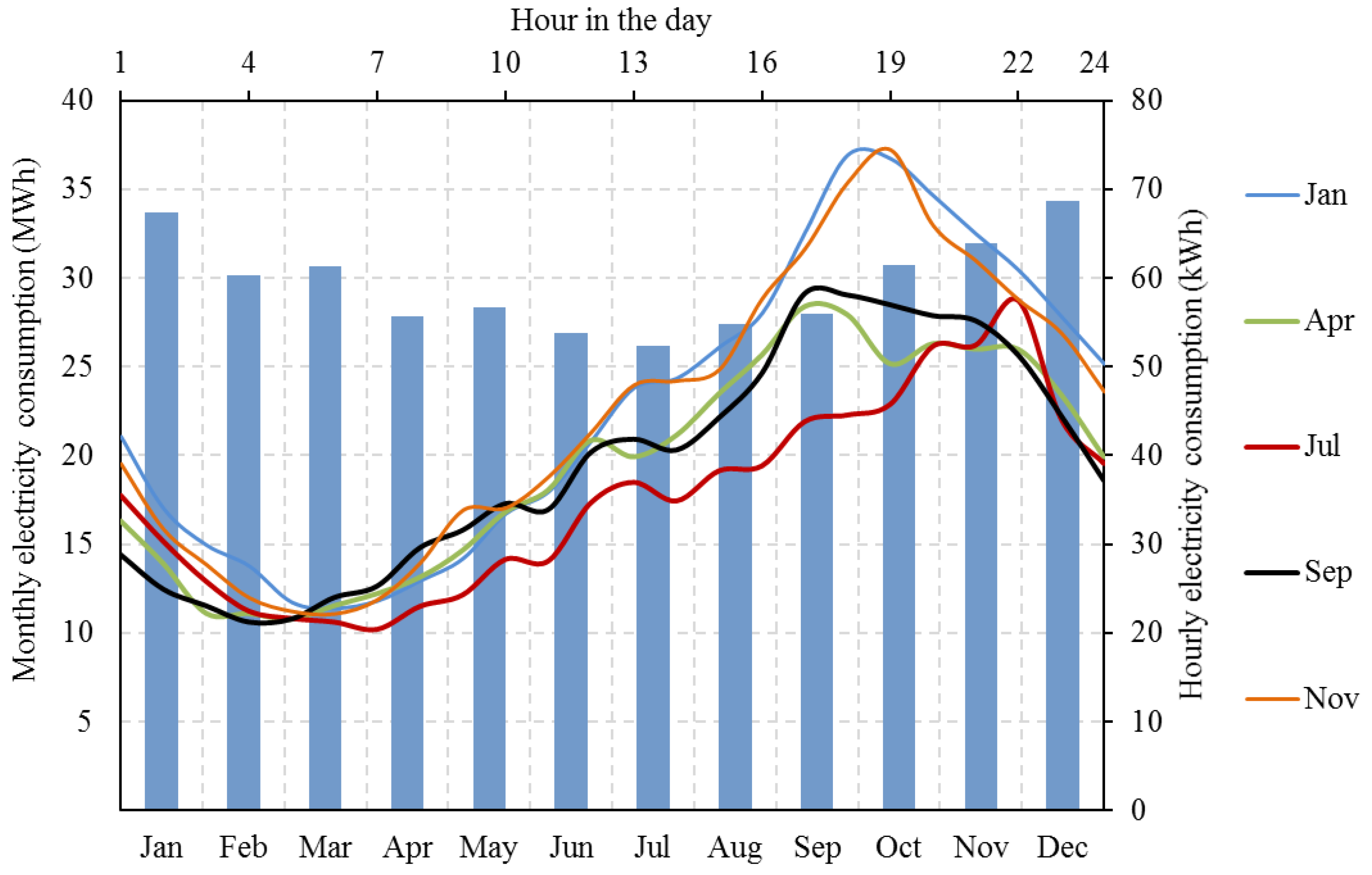
2.1. Electricity Consumption of the Case Study
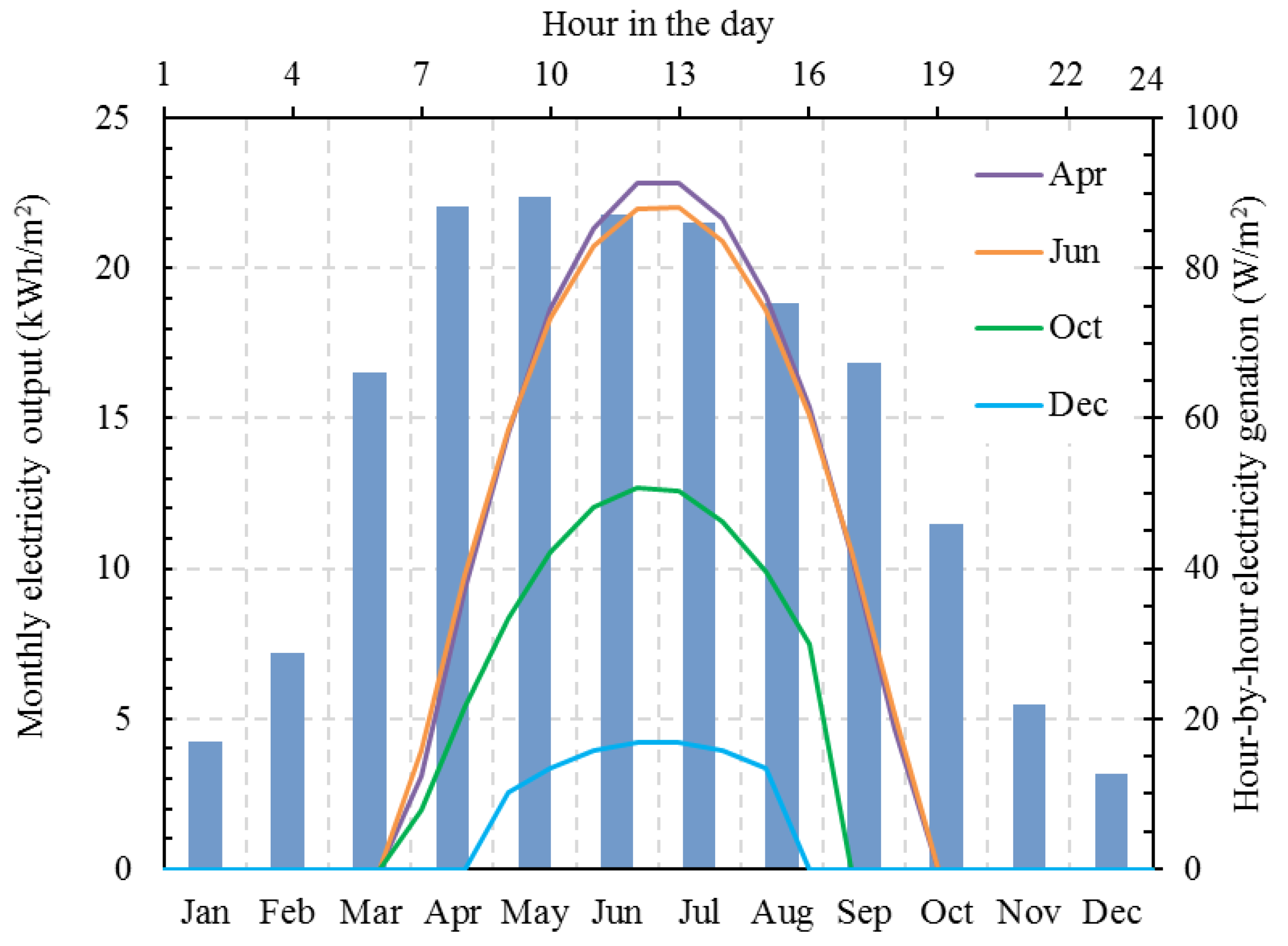
2.2. Determination of Available Solar Energy
2.3. Design of the System
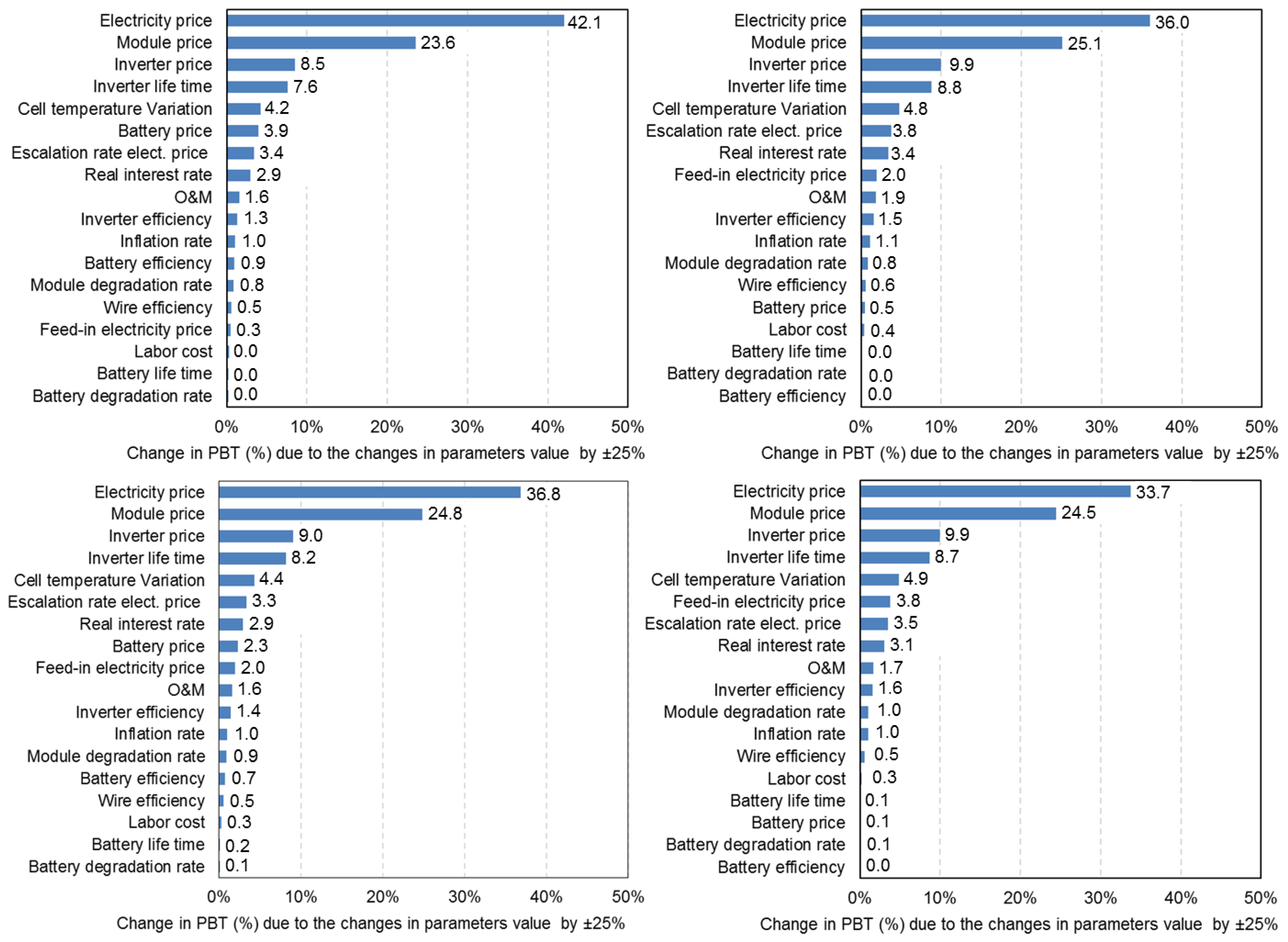
2.4. Sensitivity Analysis
3. Results and Discussion
4. Conclusions
Author Contributions
Funding
Conflicts of Interest
References
- Clerici, A.; Alimonti, G. World energy resources. EPJ Web Conf. 2015, 98, 01001. [Google Scholar] [CrossRef]
- Molar-Candanosa, R. 2015 State of the Climate: Carbon Dioxide; National Centers for Environmental Information: Asheville, NC, USA, 2016.
- Moomaw, W.; Yamba, F.; Kamimoto, M.; Maurice, L.; Nyboer, J.; Urama, K.; Weir, T. Introduction. In IPCC Special Report on Renewable Energy Sources and Climate Change Mitigation; IPCC: Geneva, Switzerland, 2011. [Google Scholar]
- Bilgili, M. Hourly simulation and performance of solar electric-vapor compression refrigeration system. Sol. Energy 2011, 85, 2720–2731. [Google Scholar] [CrossRef]
- Wrobel, J.; Sanabria Walter, P.; Schmitz, G. Performance of a solar assisted air conditioning system at different locations. Sol. Energy 2013, 92, 69–83. [Google Scholar] [CrossRef]
- Lang, T.; Ammann, D.; Girod, B. Profitability in absence of subsidies: A techno-economic analysis of rooftop photovoltaic self-consumption in residential and commercial buildings. Renew. Energy 2016, 87 Pt 1, 77–87. [Google Scholar] [CrossRef]
- Nyholm, E.; Goop, J.; Odenberger, M.; Johnsson, F. Solar photovoltaic-battery systems in Swedish households—Self-consumption and self-sufficiency. Appl. Energy 2016, 183, 148–159. [Google Scholar] [CrossRef]
- EIA (Energy Information Administration). Annual Energy Outlook; DOE/EIA-0383 (2010); EIA (Energy Information Administration): Washington, DC, USA, 2016.
- Taylor, M.; Daniel, K.; Ilas, A.; So, E. Renewable Power Generation Costs in 2014; International Renewable Energy Agency: Masdar City, Abu Dhabi, UAE, 2015. [Google Scholar]
- Hill, J.S. GTM Forecasting More Than 85 Gigawatts of Solar PV to Be Installed in 2017|CleanTechnica; CleanTechnica Comment Policy: Melbourne, Australia, 2017; Volume 2017. [Google Scholar]
- Cucchiella, F.; D’Adamo, I.; Gastaldi, M. The economic feasibility of residential energy storage combined with PV panels: The role of subsidies in Italy. Energies 2017, 10, 1434. [Google Scholar] [CrossRef]
- Luthander, R.; Widén, J.; Nilsson, D.; Palm, J. Photovoltaic self-consumption in buildings: A review. Appl. Energy 2015, 142, 80–94. [Google Scholar] [CrossRef]
- Thygesen, R.; Karlsson, B. Simulation and analysis of a solar assisted heat pump system with two different storage types for high levels of PV electricity self-consumption. Sol. Energy 2014, 103, 19–27. [Google Scholar] [CrossRef]
- Luthander, R.; Widén, J.; Munkhammar, J.; Lingfors, D. Self-consumption enhancement and peak shaving of residential photovoltaics using storage and curtailment. Energy 2016, 112, 221–231. [Google Scholar] [CrossRef]
- Mulder, G.; Ridder, F.D.; Six, D. Electricity storage for grid-connected household dwellings with PV panels. Sol. Energy 2010, 84, 1284–1293. [Google Scholar] [CrossRef]
- Castillo-Cagigal, M.; Caamaño-Martín, E.; Matallanas, E.; Masa-Bote, D.; Gutiérrez, A.; Monasterio-Huelin, F.; Jiménez-Leube, J. PV self-consumption optimization with storage and Active DSM for the residential sector. Sol. Energy 2011, 85, 2338–2348. [Google Scholar] [CrossRef]
- Kharseh, M.; Wallbaum, P.H. The effect of different working parameters on the optimal size of a battery for grid-connected PV systems. Energy Procedia 2017, 122, 595–600. [Google Scholar] [CrossRef]
- Klingler, A.-L.; Schuhmacher, F. Residential photovoltaic self-consumption: Identifying representative household groups based on a cluster analysis of hourly smart-meter data. Energy Effic. 2018, 11, 1689–1701. [Google Scholar]
- Islam, H.; Mekhilef, S.; Shah, N.B.M.; Soon, T.K.; Seyedmahmousian, M.; Horan, B.; Stojcevski, A. Performance evaluation of maximum power point tracking approaches and photovoltaic systems. Energies 2018, 11, 365. [Google Scholar] [CrossRef]
- Subramani, G.; Ramachandaramurthy, V.K.; Padmanaban, S.; Mihet-Popa, L.; Blaabjerg, F.; Guerrero, J.M. Grid-tied photovoltaic and battery storage systems with Malaysian electricity tariff—A review on maximum demand shaving. Energies 2017, 10, 1884. [Google Scholar] [CrossRef]
- Hesse, H.C.; Martins, R.; Musilek, P.; Naumann, M.; Truong, C.N.; Jossen, A. Economic optimization of component sizing for residential battery storage systems. Energies 2017, 10, 835. [Google Scholar] [CrossRef]
- Bouly de Lesdain, S. The photovoltaic installation process and the behaviour of photovoltaic producers in insular contexts: The French island example (Corsica, Reunion Island, Guadeloupe). Energy Effic. 2018, 1–12. [Google Scholar] [CrossRef]
- Yoon, K.; Yun, G.; Jeon, J.; Kim, K.S. Evaluation of hourly solar radiation on inclined surfaces at Seoul by Photographical Method. Sol. Energy 2014, 100, 203–216. [Google Scholar] [CrossRef]
- Duffie, J.A.; Beckman, W.A. Solar Engineering of Thermal Processes; Wiley: Hoboken, NJ, USA, 2006. [Google Scholar]
- El Chaar, L.; Lamont, L.A. Global solar radiation: Multiple on-site assessments in Abu Dhabi, UAE. Renew. Energy 2010, 35, 1596–1601. [Google Scholar] [CrossRef]
- Basunia, M.A.; Yoshiob, H.; Abec, T. Simulation of solar radiation incident on horizontal and inclined surfaces. J. Eng. Res. 2012, 9, 27–35. [Google Scholar] [CrossRef]
- Al-Sabounchi, A.M.; Yalyali, S.A.; Al-Thani, H.A. Design and performance evaluation of a photovoltaic grid-connected system in hot weather conditions. Renew. Energy 2013, 53, 71–78. [Google Scholar] [CrossRef]
- Al-Khawaja, M.J. Determination and selecting the optimum thickness of insulation for buildings in hot countries by accounting for solar radiation. Appl. Therm. Eng. 2004, 24, 2601–2610. [Google Scholar] [CrossRef]
- Tukiainen, M. Sunrise, Sunset, Dawn and Dusk Times around the World. Available online: www.gaisma.com (accessed on 14 June 2018).
- METEONORM Global Meteorological Database for Engineers, Planners and Education; V7.0.22.8; Meteotest Genossencschaft: Bern, Switzerland, 2004.
- Das, U.K.; Tey, K.S.; Seyedmahmoudian, M.; Idna Idris, M.Y.; Mekhilef, S.; Horan, B.; Stojcevski, A. SVR-based model to forecast PV power generation under differentweather conditions. Energies 2017, 10, 876. [Google Scholar] [CrossRef]
- SAM 2016.3.14 System Advisor Model Version 2016.3.14 (SAM 2016.3.14); National Renewable Energy Laboratory: Golden, CO, USA. Available online: https://sam.nrel.gov/content/downloads (accessed on 31 October 2016).
- Harder, E.; Gibson, J.M. The costs and benefits of large-scale solar photovoltaic power production in Abu Dhabi, United Arab Emirates. Renew. Energy 2011, 36, 789–796. [Google Scholar] [CrossRef]
- Khalid, A.; Junaidi, H. Study of economic viability of photovoltaic electric power for Quetta—Pakistan. Renew. Energy 2012, 50, 253–258. [Google Scholar] [CrossRef]
- Chandel, M.; Agrawal, G.D.; Mathur, S.; Mathur, A. Techno-economic analysis of solar photovoltaic power plant for garment zone of Jaipur city. Case Stud. Therm. Eng. 2014, 2, 1–7. [Google Scholar] [CrossRef]
- Dalenbäck, J. (Jan-Olof Dalenbäck, Professor in Building Services Engineering/Project manager CIT Energy Management AB). Personal communication, 2017.
- Paudel, A.M.; Sarper, H. Economic analysis of a grid-connected commercial photovoltaic system at Colorado State University-Pueblo. Energy 2013, 52, 289–296. [Google Scholar] [CrossRef]
- Kaplanis, S.; Kaplani, E. Energy performance and degradation over 20 years performance of BP c-Si PV modules. Simul. Model. Pract. Theory 2011, 19, 1201–1211. [Google Scholar] [CrossRef]
- CIA World Factsbook. The world Factbook: Sweden. Available online: https://www.cia.gov/library/publications/the-world-factbook/geos/print_sw.html (accessed on 15 July 2016).
- Skoczek, A.; Sample, T.; Dunlop, E.D. The results of performance measurements of field-aged crystalline silicon photovoltaic modules. Prog. Photovolt. Res. Appl. 2009, 17, 227–240. [Google Scholar] [CrossRef]
- Sánchez-Friera, P.; Piliougine, M.; Pelaez, J.; Carretero, J.; Sidrach de Cardona, M. Analysis of degradation mechanisms of crystalline silicon PV modules after 12 years of operation in Southern Europe. Prog. Photovolt. Res. Appl. 2011, 19, 658–666. [Google Scholar] [CrossRef]
- Flowers, M.E.; Smith, M.K.; Parsekian, A.W.; Boyuk, D.S.; McGrath, J.K.; Yates, L. Climate impacts on the cost of solar energy. Energy Policy 2016, 94, 264–273. [Google Scholar] [CrossRef]
- Eurostat Statistics Explained Electricity Prices for Household Consumers; Eurostat Statistics Explained: Luxembourg, 2016.
- The Global Economy Sweden: Real Interest Rate; The Global Economy: Atlanta, GA, USA, 2016.
- Tom, J.; Alice, L. (JA Energy Co., Limited). Personal communication, September 2016.
- Passer, A.; Ouellet-Plamondon, C.; Kenneally, P.; John, V.; Habert, G. The impact of future scenarios on building refurbishment strategies towards plus energy buildings. Energy Build. 2016, 124, 153–163. [Google Scholar] [CrossRef]


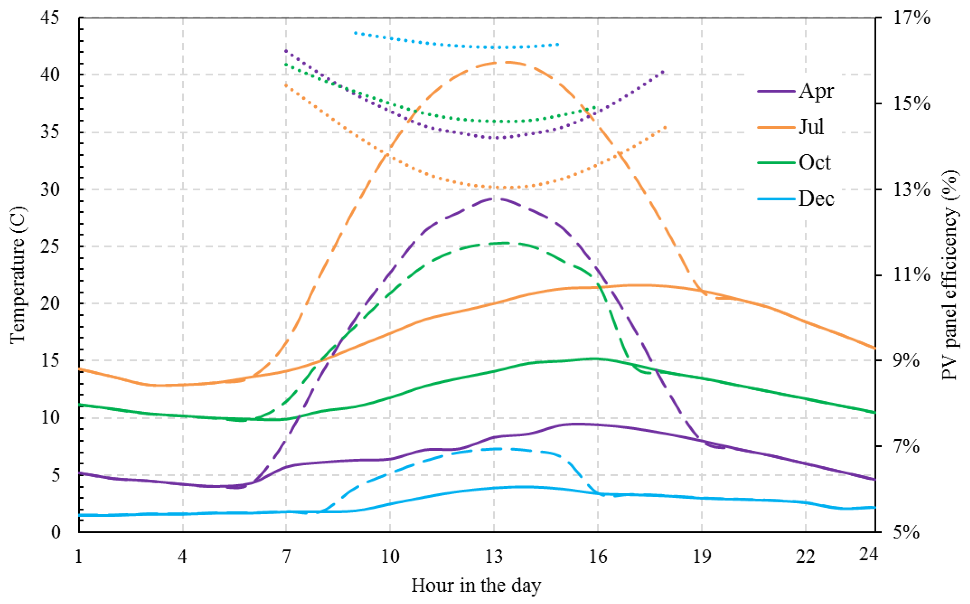
 ) outdoor air temperature, (
 ) the corresponding cell temperature of the PV module, along with (
 ) the matching PV panel efficiency.
) outdoor air temperature, () the corresponding cell temperature of the PV module, along with () the matching PV panel efficiency.
) the matching PV panel efficiency.
) outdoor air temperature, () the corresponding cell temperature of the PV module, along with () the matching PV panel efficiency.
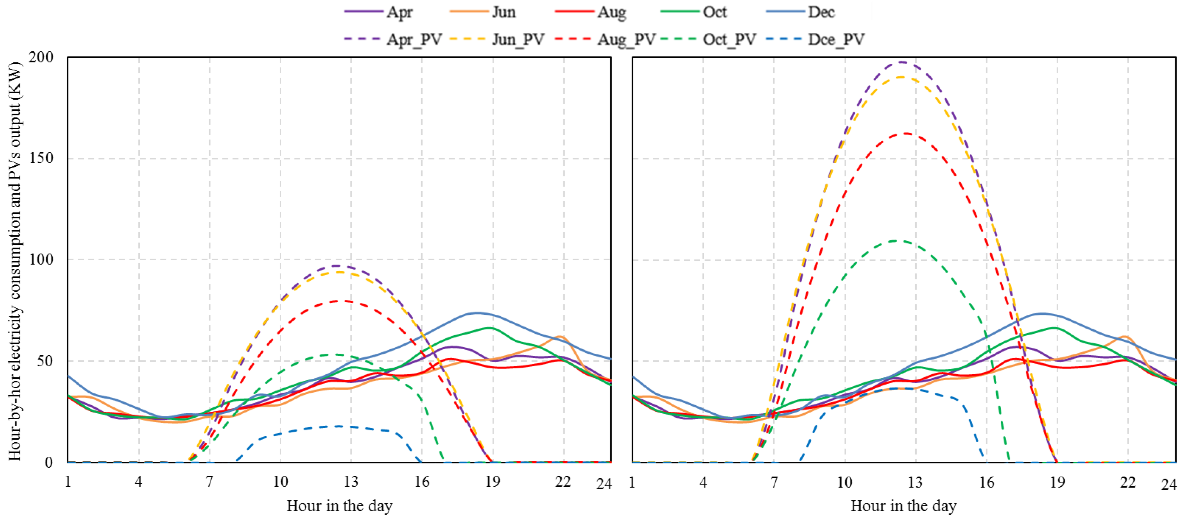
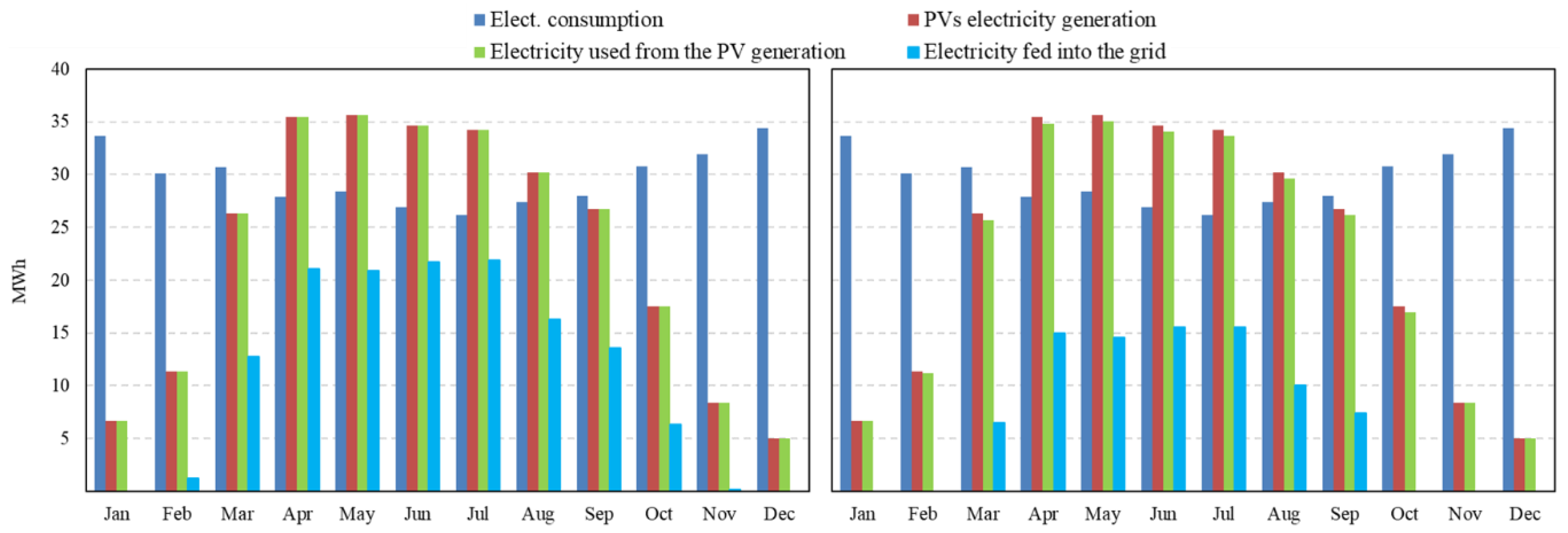
 ) energy needs of the buildings and, () the power output of the PV system of 50% saving target (left), and 100% saving target (right).
) energy needs of the buildings and, () the power output of the PV system of 50% saving target (left), and 100% saving target (right).
) energy needs of the buildings and, () the power output of the PV system of 50% saving target (left), and 100% saving target (right).


| Factor | Value |
|---|---|
| Fill factor (FF) | 0.748 |
| Derating factor | 0.891 |
| Short circuit current (A) | 9.48 |
| Open circuit voltage (V) | 46.1 |
| Voltage temperature coefficient (%/C) | −0.304 |
| Nominal operating temperature (C) | 46.0 |
| Panel capacity (W) | 325 |
| Panel price (US$) | 310 |
| Area (m2) | 1.995 |
| Factor | Value | Factor | Value | Factor | Value |
|---|---|---|---|---|---|
| inflation rate | 0.79% | Module degradation rate | 1%/y | labor cost | 18 $/kW |
| real interest rate | 2.5% | Battery degradation rate | 1%/y | Operation | 10 $/kW·y |
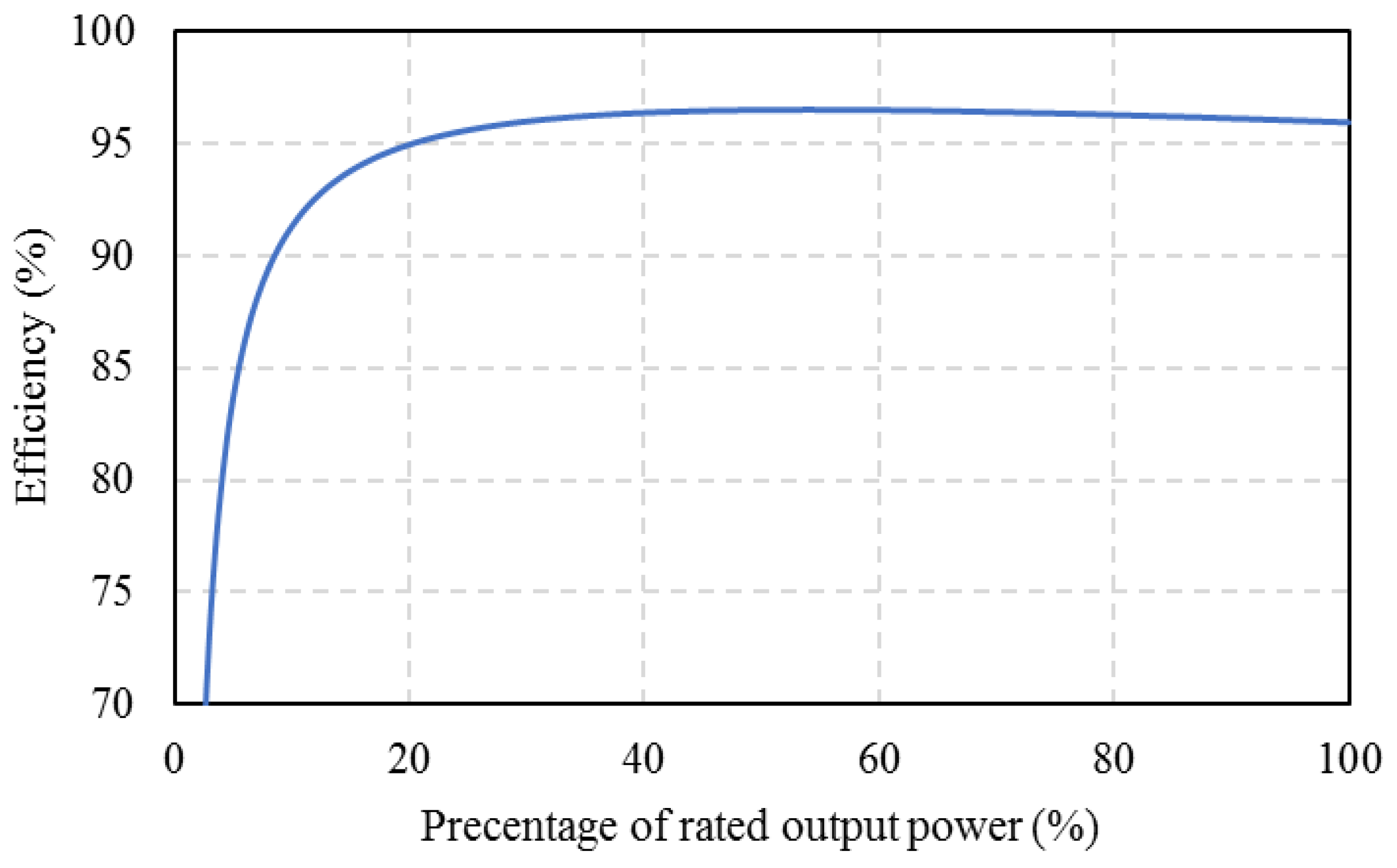
| Elec. price | 20.7 ₵/kWh | Inverter lifetime | 9 y | Inverter efficiency | Figure 3 |
| Feed-in tariff | 6.7 ₵/kWh | Battery lifetime | 8 y | Battery efficiency | 90% |
| Elec. price escalation rate | 2.3% | Lifetime of the project | 25 y | Wire efficiency | 98% |
| Module price | Table 1 | Inverter price | 322 $/kW | Battery price | 128.3 $/kWh |
| - | Cell temperature | ||||
| Factor | Range | Factor | Range |
|---|---|---|---|
| Inflation rate | 1.4%–2.4% | labor cost | 13.3–22.5 |
| Real interest rate | 0.75%–1.25% | O&M | 7.5–12.5 |
| Escalation rate of elect. | 0.75%–1.25% | module price | 93.75–156.25 |
| module degradation rate | 0.75%–1.25% | Inverter price | 241.5–402.5 |
| Cell tempe. corrector | ±25% | Electricity price | 6.9–11.6 |
| Wire efficiency | 97.5%–98.5% | Feed-in tariff | 6.9–11.6 |
| Inverter efficiency | (1 ± 25%) x each single data point in Figure 3 | Inverter lifetime | 7.5–12.5 |
© 2018 by the authors. Licensee MDPI, Basel, Switzerland. This article is an open access article distributed under the terms and conditions of the Creative Commons Attribution (CC BY) license (http://creativecommons.org/licenses/by/4.0/).
Share and Cite
Kharseh, M.; Wallbaum, H. How Adding a Battery to a Grid-Connected Photovoltaic System Can Increase its Economic Performance: A Comparison of Different Scenarios. Energies 2019, 12, 30. https://doi.org/10.3390/en12010030
Kharseh M, Wallbaum H. How Adding a Battery to a Grid-Connected Photovoltaic System Can Increase its Economic Performance: A Comparison of Different Scenarios. Energies. 2019; 12(1):30. https://doi.org/10.3390/en12010030
Chicago/Turabian StyleKharseh, Mohamad, and Holger Wallbaum. 2019. "How Adding a Battery to a Grid-Connected Photovoltaic System Can Increase its Economic Performance: A Comparison of Different Scenarios" Energies 12, no. 1: 30. https://doi.org/10.3390/en12010030
APA StyleKharseh, M., & Wallbaum, H. (2019). How Adding a Battery to a Grid-Connected Photovoltaic System Can Increase its Economic Performance: A Comparison of Different Scenarios. Energies, 12(1), 30. https://doi.org/10.3390/en12010030