Abstract
To improve the energy efficiency of a mobile robot, a novel energy modeling method for mobile robots is proposed in this paper. The robot can calculate and predict energy consumption through the energy model, which provides a guide to facilitate energy-efficient strategies. The energy consumption of the mobile robot is first modeled by considering three major factors: the sensor system, control system, and motion system. The relationship between the three systems is elaborated by formulas. Then, the model is utilized and experimentally tested in a four-wheeled Mecanum mobile robot. Furthermore, the power measurement methods are discussed. The energy consumption of the sensor system and control system was at the milliwatt level, and a Monsoon power monitor was used to accurately measure the electrical power of the systems. The experimental results showed that the proposed energy model can be used to predict the energy consumption of the robot movement processes in addition to being able to efficiently support the analysis of the energy consumption characteristics of mobile robots.
1. Introduction
Robotics is undergoing a major transformation in scope and dimension. From a largely dominant industrial focus, robotics is rapidly expanding into human environments and is vigorously engaged in new challenges [1,2]. In order to work better in complex situations, these robots are mobile and driven by batteries [3]. Mobile robots are widely used in modern manufacturing systems, while their use is also extending into human daily life [4].
Mobile robots are limited by heavy and expensive batteries, which makes energy efficiency a key constraint on robot performance. Thus, modeling and managing energy consumption is of vital importance to predict the lifetime and range of autonomous platforms. It is of great significance to study the energy consumption of mobile robots [5,6]. The energy problem of mobile robots has been paid more attention in order to meet requirements of reducing energy consumption. The energy consumption modeling of mobile robots [7] based on mathematical formulas can be more scientific to study the influence of operation states on energy consumption, which provides a guide to facilitate energy-efficient strategies [8]. Firstly, the robot itself can clearly understand the energy required for the robot’s motion and the specific energy consumption of each part; therefore, the energy consumption can be reduced according to different situations and the existing energy support can be estimated. Still, recent publications have adopted very different methods when it comes to the calculation of energy consumption. Many authors have attempted to achieve this through modifications in trajectory planning, control, or mechanical design [9,10,11,12,13].
A novel method of energy consumption modeling is proposed in this paper. The method involves dividing the energy consumption of the robot into three parts: the sensor system, control system, and motion system. The block diagram of the system is shown in Figure 1. Figure 1a represents the electrical energy transmission and Figure 1b represents the signal transmission during the robot’s work.
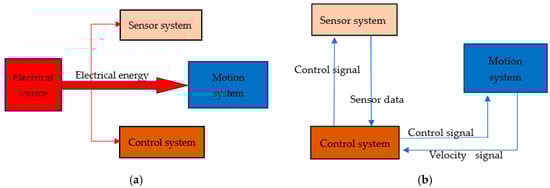
Figure 1.
Block diagram of the system. (a) Electrical energy transmission; (b) Signal transmission.
The electrical power measurement tools accurately measure the specific electrical power of the three parts and then give a complete mathematical formula to summarize the energy consumption of the robot in various situations.
This model was utilized and experimentally tested in a four-wheeled Mecanum mobile robot. These types of robots can move sideways, turn on the spot, and follow complex trajectories [14]. These robots are capable of easily performing tasks in environments with static and dynamic obstacles and narrow aisles [15]. The electrical power of the sensor system and control system was at the milliwatt level, and a Monsoon power monitor was used to accurately measure the electrical power of the systems. The electrical power of the motion system was at the watt level, and a Rigol DP1308A programmable direct current (DC) power supply (RIGOL Technology Co., Ltd., Beijing, China) was used to measure the motion system.
2. Related Works
With the aim of energy consumption minimization in robots, many published works have described effective methods to achieve this goal.
An energy modeling method by measuring the total power for an industry robot was proposed by Xu et al. [8]. This method avoids the problem of directly measuring relevant parameters inside the robot. The main content of this method is joint torque modeling, and the parameter estimation is one of the most important steps in the process of the torque modeling.
Verstraten et al. [9] studied how well different modeling approaches commonly found in the literature can predict the energy consumption of a geared DC motor performing a dynamic task. The results from their work serve to aid designers in deciding which elements to include in their model, whether their purpose is to compare designs or to obtain an actual estimate of the consumed power.
In References [16,17], energy optimization was investigated by hardware replacements. Using low power hardware can reduce the overall electrical energy consumption of the robot.
Bukata et al. [18] studied the energy optimization of industrial robotic cells, which is essential for sustainable production in the long term. A holistic approach that considers a robotic cell as a whole robot was proposed in order to minimize energy consumption. The mathematical model, which considers various robot speeds, positions, power-saving modes, and alternative orders of operations, can be transformed into a mixed-integer linear programming formulation that is, however, suitable only for small instances. To optimize complex robotic cells, a hybrid heuristic accelerated method using multicore processors and the Gurobi simplex method for piecewise linear convex functions was implemented.
A European Commission-funded research project developed a novel generation method for energy-efficient direct current (DC)-supplied robots to overcome current industrial robots’ energetic limitations and to leverage the exchange, storage, and recovery of energy at the factory level. The novel DC-supplied robots developed with the AREUS project (www.areus-project.eu) may enable DC industrial smart grids with full regenerative bidirectional DC power flow and the seamless integration of renewable energy sources [19].
Many research works have achieved the goal of saving energy through trajectory optimization [20,21,22]. Xie. et al. studied the online minimum-energy trajectory planning of both nonholonomic and holonomic drives on a straight-line path. Their energy cost function is the sum energy drawn from the onboard batteries and includes energy dissipation by the motor armature, the energy over-coming frictions, and the kinetic energy of the robot. A closed-form solution of the minimum-energy rotational velocity trajectory was found using Pontryagin’s minimum principle, and the minimum-energy translational velocity trajectory was found using a new researching algorithm. Their results showed that following the same straight-line path via different velocity profiles consumed different amounts of energy. However, their studies were restricted to straight-line paths and stationary states in the beginning and at the end, and hence became less practical for autonomous navigation [21]. Bartlett et al. proposed a probabilistic, data-driven approach to estimating the energy consumption of a mobile robot on a set of trajectories, whether they have been traversed or not. In particular, the robot was treated as a black box, thereby removing the reliance on often unavailable system characteristics. They measured the consumption directly on the routes traversed and utilized features derived from publicly available maps to extrapolate to energy consumption on real-world routes [22]. A self-supervised approach was presented which considers terrain geometry and soil types. In particular, this paper analyzed soil types which affect energy usage models, then proposed a prediction scheme based on terrain type recognition and simple consumption modeling [23].
Many articles have discussed the energy consumption of a robot’s mechanical structure [24,25,26]. The total energy consumption of the robot consists of the energy consumption of the mechanism and the subsidiary electrical power loss. Caponetto et al. [27] used a neural network to develop a nonlinear dynamical model of a fuel cell stack that can be exploited as a component of complex control systems to manage the energy flows between the fuel cell stack, battery pack, auxiliary systems, and electric engine.
3. Practical Energy Modeling Method
In order to optimize the energy consumption model, researchers focused on single-component as well as system-level energy optimization through dynamic power management. The energy consumption model of the mobile robot is divided to three parts: the sensor system, control system, and motion system.
3.1. Energy Consumption of the Sensor System
Firstly, the energy consumption of the sensor part is almost stable. Thus, the energy consumption of the sensor part is multiplied by the electrical power and time.
is the electrical power of the sensor system and is the electrical energy consumption.
Secondly, the energy consumption of sensors is related to the speed of the robot. Because the sensor’s transmission speed is fast, it can quickly model the surrounding environment. The speed of a mobile robot changes from low to high. If the robot is moving slowly, instead of working all the time, the sensor can wait for the robot to move for a while and then re-model the surrounding environment. Similarly, when the robot is in a standby state, there is no need to model its surroundings, so the sensor is dormant. When the robot reaches its maximum speed, the speed is very fast, and the surrounding environment changes very quickly, thus the sensor needs to work continuously. Thus, the overall energy consumption of the sensor is proportional to the speed.
is the maximum speed of the mobile robot. Obviously, this method can reduce the energy consumption of sensors compared with the scenario in which the sensors are working all the time.
3.2. Energy Consumption of the Control System
The energy consumption of the control system depends on the power of the control circuit boards [21], which is related to the running state of the robot. The energy modeling of the control system is mainly divided into the following three parts: the energy consumption in the standby state, the energy consumption when the robot just starts to move, and the energy consumption when the robot runs smoothly.
represents the power of the control part in the standby state. It is determined that the control system only accepts the signal of the sensor during standby, so the power is a constant. is the starting factor of the robot; this factor determines the energy demand for the controller during the start of the robot. is the rate of change of the current moment and t is the time when the robot starts moving.
3.3. Energy Consumption of the Motion System
Concerning the motion system, the energy consumption can be divided into four parts: the traction energy consumption, increase of kinetic energy, friction energy dissipation, and energy dissipated in thermal form. The motion of a robot is divided into three stages: standby, startup, and stable operation. The power is constant in the standby stage. In the startup stage, there is an instantaneous pulse, which is needed to send the start signal to the electric motors. When a robot moves, it enters the stable operation stage.
is the energy consumed to attain and sustain robotic motion, while the motion power is motion-dependent [14]. is the kinetic energy of the robot, is the mass of the mobile robot, and is the speed of the current moment of the robot.
is the friction dissipation during the movement of the robot; is the friction coefficient between the wheel and the ground.
is the energy dissipation as heat in the armatures of motors; and are the time-heat constants; is the speed-heat constant of the robot.
is the mechanical dissipation caused by overcoming the friction torque in the actuators. is the drag coefficient of the robot itself; the coefficient is only related to the robot itself. is the vibration velocity coefficient of the robot.
Consequently, the energy behavior of the motion system can be expressed by Equation (9):
The specific parameter values of Equations (5)–(8) are listed in Table 1. The value of each parameter was obtained through the estimation method. The energy model was simulated through MATLAB software. The graphics in Figure 2, Figure 3, and Figure 4 represent the simulation results of the model.

Table 1.
Value of each parameter.
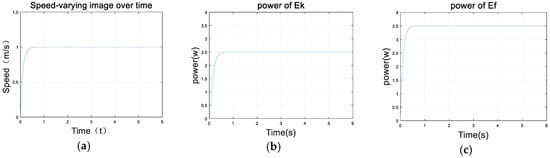
Figure 2.
Speed, , and change versus time. (a) Speed change versus time; (b) Kinetic energy changes; (c) Friction dissipation.
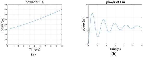
Figure 3.
Thermal dissipation and mechanical dissipation. (a) Thermal dissipation; (b) Mechanical dissipation.
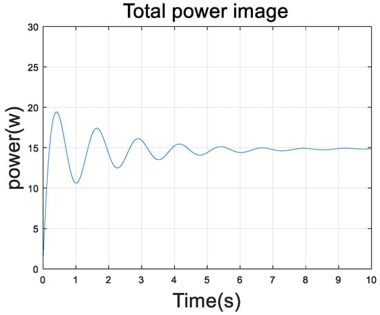
Figure 4.
Total power of the motion system.
The speed change of the robot is shown as a function of time in Figure 2a and the maximum is 1 m per second. Bringing the speed value v into Equation (5), the kinetic energy of the robot can be calculated as shown in Figure 2b. Bringing the speed value v into Equation (6), the friction dissipation is shown as in Figure 2c.
Figure 3a shows the energy dissipation as heat. Figure 3b shows the variation of the mechanical energy consumption over time.
In the end, we can obtain the total power of the motion system from Equation (4) as shown in Figure 4, and the power is convergent.
3.4. The Connection between the Three Systems
The energy consumption model of mobile robots consists of three parts: the sensor system, control system, and motion system. Concerning the energy consumption, there are mutual constraints between the three systems. Firstly, when a robot is in a standby state, the energy consumption of the control part, the moving part, and the sensor part is very low. Thus, the total energy consumption can be considered as the sum of the idle energy () and the motional energy ().
When a robot starts to move, the control system of the robot starts sending and receiving data and it takes time to accelerate from zero to maximum speed. At first the robot does not move very fast, so the sensors do not need to be working all the time. The higher the speed, the higher electrical power required by the sensor system. Once the robot starts to move, the control system of the robot must keep working, as this system is responsible for accepting the sensor signals as well as motion feedback signals, calculating data, and sending out control signals. Thus, the power required by the control system will increase. As the speed of the robot increases, the frequency of data received, processed, and transmitted by robots will increase, and more power will be required by the systems. When the robot reaches its maximum speed, sensor and motion systems work with the highest power.
3.5. Energy Consumption of the Whole System
Because mobile robots are driven by lithium batteries, following the basic relationship between power and energy, we can calculate the electrical energy consumption () from the source power () by the integration of time [9].
4. Electrical Energy Consumption Evaluation and Result Analysis
The model was utilized and experimentally tested in a four-wheel-drive Mecanum mobile robot, as shown in Figure 5.
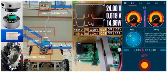
Figure 5.
Four-wheel-drive Mecanum mobile robot and power measurement.
A Monsoon solution AAA10F power monitor (Monsoon Solutions Inc., Bellevue, WA, USA) was used to measure the electrical power of the sensor and controller. A Rigol DP1308A (RIGOL Technology Co., Ltd., Beijing, China) was used to measure the electrical power of the motion system as well as the total power consumption. The power of the system can also be monitored by measuring the real-time voltage and current of the battery.
The experimental environment was a common laboratory environment. The chassis of the McNam’s wheeled car moved across the ceramic tile floor of the laboratory. The experimental method was as follows: a mobile phone app was used to remotely move the robot forward 4 m; then, the energy consumption of this process was calculated.
4.1. Power Measurement of the Sensor System
Measuring the power of the sensor using a power monitor, as shown in Figure 6b, the power consumption of the sensor was between 600 and 700 mW. It exhibited a stable curve with almost no fluctuation. This result which is shown in Figure 7 conforms to the sensor power model.
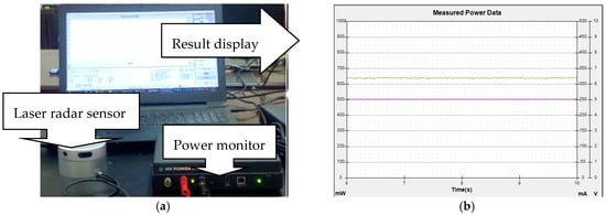
Figure 6.
Power measurement of the sensor. (a) Sensor power measurement; (b) Power result display.
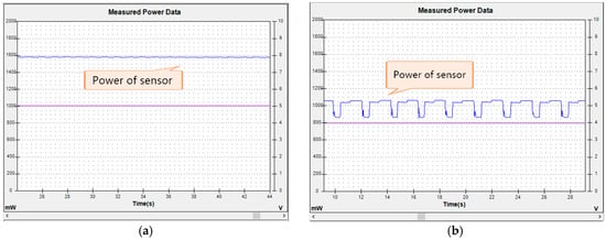
Figure 7.
Sensor system power. (a) Sensor power sampled every 0.02 s; (b) Sensor power sampled every 0.04 s.
Comparing the power from different sampling frequencies, it was found that when the sampling frequency was reduced, the power of the sensor also decreased.
As shown in Table 2, the lower the robot speed, the lower the power of the sensor system, and the error between the measured value and the modeled value was within 7%.
Table 2.
Sensor power comparison between model and measurement.
4.2. Power Measurement of the Control System
Selecting the low power control chip and interface circuit can reduce the total power of the control system. The mobile robot used an STM32F103 chip as the main control chip, as shown in Figure 8.
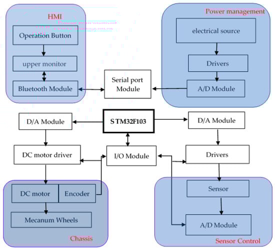
Figure 8.
Block diagram of the control system.
Figure 9 displays the power measurement of the controller board and the result. Not only hardware but also software makes a significant contribution to the overall power consumed by small-size embedded systems [28]. In order to accurately study the power situation of the control system at each stage, it needed to be ensured that there was sufficient time to sample the power. Therefore, in the setting stage, we set the acceleration of the robot to a relatively small value. Figure 10a shows the power of the control system during startup. Figure 10b shows the power of the control system after the robot runs smoothly. It was found through the comparison that the faster the acceleration, the higher the frequency of the pulse signal emitted by the control part. Thus, the pulse signal can be regarded as the acceleration signal sent by the control part to the moving part. After stabilization, the control part keeps the original power almost unchanged, but there is no pulse signal.
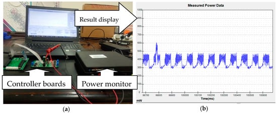
Figure 9.
Power measurement of the controller boards. (a) Control boards power measurement; (b) Power result.
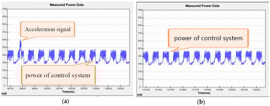
Figure 10.
Power of the control system. (a) Start process power; (b) Smooth running power.
4.3. Power Measurement of the Motion System
Accurate measurement and analysis of energy consumption are essential for the evaluation of the hardware- and software-related energy consumption of a processing system [28,29]. The model of the control system can affect the energy consumption of the whole system [30]. Therefore, the robot was set to run by a specific program, the flowchart of which is shown in Figure 11.
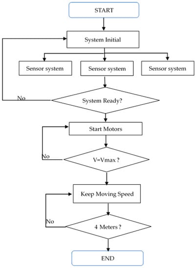
Figure 11.
Flowchart of the robot’s motion.
In order to ensure the accuracy of the experimental measurement, we set the maximum speed of the robot at 1 m/s through the program. When the speed of the robot reached 1 m/s, the robot stopped accelerating. The robot was closed-loop controlled. Photoelectric encoders on the motors measured the speed of the motor and provided feedback data in real time to the control system of the robot. When the control system detected that the speed of the robot had reached the set value, it stopped accelerating and maintained that speed. Otherwise, it continued to accelerate.
Table 3 shows the comparison between the real data we measured and the data we obtained using the proposed model. The difference between the modeled data and the actual measured data was small, reaching no more than 3%.
Table 3.
Motion power comparison between model and measurement.
Figure 12 shows the power of the motion system obtained by the model. The power changed rapidly at the beginning, then the power converged to a smaller interval, and remained almost constant in the end.
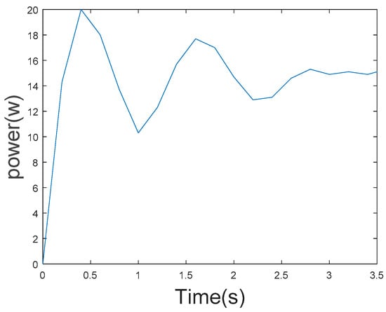
Figure 12.
Power of the motion system obtained by the model.
In Table 4, the maximum deviation means the degree of deviation from the maximum motion power and the stable deviation means the degree of deviation from the stable motion power when the robot runs smoothly. The robot’s motion electrical power tends to stabilize over time.
Table 4.
Motion electrical power.
4.4. Robot’s Total Power Comparison between the Model and Measurements
Table 5 shows the results of the five experiments. DP1308A was employed to record the power consumption as the robot was run through the power meter, which was then imported into MATLAB for analysis. Ghost power represents the power of the robot when it was not moving.
Table 5.
Total power of experiment results.
As seen from Figure 13, the power calculated by the model and the actual measured power error were both within an acceptable range.
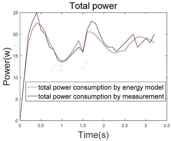
Figure 13.
Comparison between energy model and measurement.
Figure 14a shows the change in the percentage of electrical power of the three parts of the robot from the startup to 1 m/s of robot movement. Figure 14b shows the electrical power percentage of the robot’s three parts during the smooth-running state of the robot. The proportion of the motion system to the total power far exceeds that of the sensor system and control system.
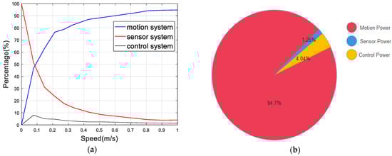
Figure 14.
Percentage of power. (a) Power percentage of the three systems; (b) Smooth running power percentage.
5. Conclusions and Future Work
The energy modeling method for mobile robots presented in this paper can be used to calculate and predict energy consumption, providing a guide to facilitate energy-efficient strategies as well as avoiding action obstacles due to lack of energy. The operation of robots can be divided into three states: standby, startup, and running. Compared with the other modeling methods, this model does not consider the path of the robot. The electrical power calculation method is related to the speed of the robot and the characteristics of the robot itself. By dividing the energy consumption of the robot into three parts, the model can be simplified. Therefore, very complicated parameters in the process of motion are not needed, and the calculation of electrical power becomes very simple. It is convenient for us to put this model into our program so that the robot has the ability of self-perception. Through our model, we established the relationship and connection among the three parts, which can make the model of the robot more complete.
Experiments showed that the power model created in this paper is feasible and effective. However, the experiments were carried out on horizontal roads only. The operation of robot involves stopping, accelerating, slowing down, turning, movement uphill and downhill, and so on, all of which is not entirely covered by the proposed energy model. Thus, further research should aim to complete the energy model according to all robot actions, using a better and more comprehensive experimental field. Moreover, the battery energy model is very important and should be included in a complete energy model for mobile robots.
Author Contributions
Conceptualization, L.Z. and J.K.; Methodology, L.Z.; Software, L.H.; Validation, L.H., L.Z.; Formal Analysis, L.H.; Investigation, L.Z.; Resources, L.H.; Data Curation, L.H.; Writing-Original Draft Preparation, L.H.; Writing-Review & Editing, J.K.; Visualization, J.K.; Supervision, L.Z.; Project Administration, L.Z.; Funding Acquisition, L.Z.
Funding
This research received no external funding.
Conflicts of Interest
The authors declare no conflict of interest.
References
- Burghardt, A.; Kurc, K.; Szybicki, D.; Muszyńska, M.; Szczęch, T. Monitoring the parameters of the robot-operated quality control process. Adv. Sci. Technol. Res. J. 2017, 11, 232–236. [Google Scholar] [CrossRef]
- Cafolla, D.; Ceccarelli, M. An experimental validation of a novel humanoid torso. Robot. Auton. Syst. 2017, 91, 299–313. [Google Scholar] [CrossRef]
- Tampubolon, M.; Pamungkas, L.; Chiu, H.J.; Liu, Y.C.; Hsieh, Y.C. Dynamic Wireless Power Transfer for Logistic Robots. Energies 2018, 11, 527. [Google Scholar] [CrossRef]
- Clotet Bellmunt, E.; Martínez Lacasa, D.; Moreno Blanc, J.; Tresánchez Ribes, M.; Palacín Roca, J. Assistant Personal Robot (APR): Conception and Application of a Tele-Operated Assisted Living Robot. Sensors 2016, 16, 610. [Google Scholar] [CrossRef] [PubMed]
- Canfield, S.L.; Hill, T.W.; Zuccaro, S.G. Prediction and Experimental Validation of Power Consumption of Skid-Steer Mobile Robots in Manufacturing Environments. J. Intell. Robot. Syst. 2018, 1–15. [Google Scholar] [CrossRef]
- Chuy, O.; Collins, E.G.J.; Yu, W.; Ordonez, C. Power modeling of a skid steered wheeled robotic ground vehicle. In Proceedings of the IEEE International Conference on Robotics and Automation, Kobe, Japan, 12–17 May 2009; pp. 4118–4123. [Google Scholar] [CrossRef]
- Liu, S.; Sun, D. Modeling and experimental study for minimization of energy consumption of a mobile robot. In Proceedings of the International Conference on Advanced Intelligent Mechatronics, Kachsiung, Taiwan, 11–14 July 2012; pp. 708–713. [Google Scholar] [CrossRef]
- Xu, W.; Liu, H.; Liu, J.; Zhou, Z.; Pham, D.T. A Practical Energy Modeling Method for Industrial Robots in Manufacturing. In Challenges and Opportunity with Big Data; Monterey Workshop 2016. Lecture Notes in Computer Science; Zhang, L., Ren, L., Kordon, F., Eds.; Springer: Cham, The Netherlands, 2017; Volume 10228. [Google Scholar]
- Verstraten, T.; Furnémont, R.; Mathijssen, G.; Vanderborght, B.; Lefeber, D. Energy Consumption of Geared DC Motors in Dynamic Applications: Comparing Modeling Approaches. IEEE Robot. Autom. Lett. 2016, 1, 524–530. [Google Scholar] [CrossRef]
- Lu, B.; Jan, L.; Jan, Y.N. Control of cell divisions in the nervous system: Symmetry and asymmetry. Annu. Rev. Neurosci. 2000, 23, 531. [Google Scholar] [CrossRef] [PubMed]
- Martin, D.; Caballero, B.; Haber, R. Optimal Tuning of a Networked Linear Controller Using a Multi-Objective Genetic Algorithm. Application to a Complex Electromechanical Process. In Proceedings of the International Conference on Innovative Computing Information and Control, Dalian, China, 18–20 June 2008; Volume 91. [Google Scholar] [CrossRef]
- Haidegger, T.; Kovács, L.; Precup, R.E.; Benyó, B.; Benyó, Z.; Preitl, S. Simulation and control for telerobots in space medicine. Acta Astronaut. 2012, 81, 390–402. [Google Scholar] [CrossRef]
- Vrkalovic, S.; Teban, T.-A.; Borlea, I.-D. Stable Takagi-Sugeno fuzzy control designed by optimization. Int. J. Artif. Intell. 2017, 15, 17–29. [Google Scholar]
- Doroftei, I.; Grosu, V.; Spinu, V. Design and Control of an Omni-directional Mobile Robot. In Novel Algorithms and Techniques In Telecommunications, Automation and Industrial Electronics; Springer: Dordrecht, The Netherlands, 2008; pp. 105–110. [Google Scholar]
- Qian, J.; Zi, B.; Wang, D.; Ma, Y.; Zhang, D. The design and development of an omni-directional mobile robot oriented to an intelligent manufacturing system. Sensors 2017, 17, 2073. [Google Scholar] [CrossRef]
- Saidur, R. A review on electrical motors energy use and energy savings. Renew. Sustain. Energy Rev. 2010, 14, 877–898. [Google Scholar] [CrossRef]
- Yang, A.; Pu, J.; Wong, C.B.; Moore, P. By-pass valve control to improve energy efficiency of pneumatic drive system. Control Eng. Pract. 2009, 17, 623–628. [Google Scholar] [CrossRef]
- Bukata, L.; Sucha, P.; Hanzalek, Z.; Burget, P. Energy optimization of robotic cells. IEEE Trans. Ind. Inf. 2017, 13, 92–102. [Google Scholar] [CrossRef]
- Grebers, R.; Gadaleta, M.; Paugurs, A.; Senfelds, A.; Avotins, A.; Pellicciari, M. Analysis of the energy consumption of a novel dc power supplied industrial robot. Procedia Manuf. 2017, 11, 311–318. [Google Scholar] [CrossRef]
- Xie, L.; Henkel, C.; Stol, K.; Xu, W. Power-minimization and energy-reduction autonomous navigation of an omnidirectional Mecanum robot via the dynamic window approach local trajectory planning. Int. J. Adv. Robot. Syst. 2018, 15. [Google Scholar] [CrossRef]
- Bartlett, O.; Gurau, C.; Marchegiani, L.; Posner, I. Enabling intelligent energy management for robots using publicly available maps. In Proceedings of the 2016 IEEE/RSJ International Conference on Intelligent Robots and Systems (IROS), Daejeon, Korea, 9–14 October 2016; pp. 2224–2229. [Google Scholar] [CrossRef]
- Kang, H.; Liu, C.; Jia, Y.-B. Inverse dynamics and energy optimal trajectories for a wheeled mobile robot. Int. J. Mech. Sci. 2017, 134, 576–588. [Google Scholar] [CrossRef]
- Otsu, K.; Kubota, T. Energy-Aware Terrain Analysis for Mobile Robot Exploration. In Field and Service Robotics; Springer International Publishing: New York, NY, USA, 2016. [Google Scholar]
- Halevi, Y.; Carpanzano, E.; Montalbano, G.; Koren, Y. Minimum energy control of redundant actuation machine tools. CIRP Ann.-Manuf. Technol. 2011, 60, 433–436. [Google Scholar] [CrossRef]
- Lee, G.; Park, S.; Lee, D.; Park, F.C.; Jeong, J.I.; Kim, J. Minimizing energy consumption of parallel mechanisms via redundant actuation. IEEE/ASME Trans. Mech. 2015, 20, 2805–2812. [Google Scholar] [CrossRef]
- Han, G.; Xie, F.; Liu, X.J. Evaluation of the power consumption of a high-speed parallel robot. Front. Mech. Eng. 2018, 13, 1–12. [Google Scholar] [CrossRef]
- Caponetto, R.; Fortuna, L.; Rizzo, A. Neural network modelling of fuel cell systems for vehicles. In Proceedings of the IEEE Conference on Emerging Technologies and Factory Automation, Catania, Italy, 19–22 September 2005; Volume 6, p. 192. [Google Scholar] [CrossRef]
- Innovation, B. Measurement of Power Consumption in Digital Systems. IEEE Trans. Instrum. Meas. 2005, 55, 1662–1670. [Google Scholar] [CrossRef]
- Laopoulos, T.; Neofotistos, P.; Kosmatopoulos, K.; Nikolaidis, S. Measurement of current variations for the estimation of software-related power consumption. IEEE Trans. Instrum. Meas. 2003, 52, 1206–1212. [Google Scholar] [CrossRef]
- Caponetto, R.; Dongola, G.; Fortuna, L. A new class of fault-tolerant systems: FPGA implementation of bio-inspired self-repairing system. In Proceedings of the 2007 Mediterranean Conference on Control & Automation, Athens, Greece, 27–29 June 2007; pp. 1–4. [Google Scholar] [CrossRef]
© 2018 by the authors. Licensee MDPI, Basel, Switzerland. This article is an open access article distributed under the terms and conditions of the Creative Commons Attribution (CC BY) license (http://creativecommons.org/licenses/by/4.0/).