Short-Term Load Forecasting in Smart Grids: An Intelligent Modular Approach

Abstract

Daily operations and planning in a smart grid require a day-ahead load forecasting of its customers. The accuracy of day-ahead load-forecasting models has a significant impact on many decisions such as scheduling of fuel purchases, system security assessment, economic scheduling of generating capacity, and planning for energy transactions. However, day-ahead load forecasting is a challenging task due to its dependence on external factors such as meteorological and exogenous variables. Furthermore, the existing day-ahead load-forecasting models enhance forecast accuracy by paying the cost of increased execution time. Aiming at improving the forecast accuracy while not paying the increased executions time cost, a hybrid artificial neural network-based day-ahead load-forecasting model for smart grids is proposed in this paper. The proposed forecasting model comprises three modules: (i) a pre-processing module; (ii) a forecast module; and (iii) an optimization module. In the first module, correlated lagged load data along with influential meteorological and exogenous variables are fed as inputs to a feature selection technique which removes irrelevant and/or redundant samples from the inputs. In the second module, a sigmoid function (activation) and a multivariate auto regressive algorithm (training) in the artificial neural network are used. The third module uses a heuristics-based optimization technique to minimize the forecast error. In the third module, our modified version of an enhanced differential evolution algorithm is used. The proposed method is validated via simulations where it is tested on the datasets of DAYTOWN (Ohio, USA) and EKPC (Kentucky, USA). In comparison to two existing day-ahead load-forecasting models, results show improved performance of the proposed model in terms of accuracy, execution time, and scalability.

1. Introduction

An existing/traditional grid system needs renovation to bridge the ever-increasing gap between demand and supply and also to meet essential challenges such as grid reliability, grid robustness, customer electricity cost minimization, etc. [1]. In this regard, recent integration of advanced communication technologies and infrastructures into traditional grids have led to the formation of so called smart grids (SGs) [2]. The national national institute of standards and technology (NIST) [3] conceptual diagram of smart grid (SG) is shown in Figure 1. This conceptual diagram can be used as a reference model for standardization works in seven SG domains: generation, transmission, distribution, end users, markets, operations, and service providers. Each domain involves one or more SG actors (e.g., devices, systems, programs, etc.) to make decisions for realizing an application based on exchange of information. Further details on each domain, its involved actors, and respective applications can be found in [3]. One of the advantages of this integration is customer engagement, which plays a key role in the economies of energy trade. In other words, the old concept of uni-directional energy flow is replaced by the new and smart concept of bi-directional energy flow—transformation from traditional consumer to a smart prosumer [4].

The resulting/new grid, integrated with advanced metering infrastructure, faces many challenges such as [5]: (i) designing new techniques to meet the load while not increasing the generation capacity; and (ii) devising new ways/policies to ensure customer engagement with utility. When installing new technologies, utilities aim for a maximum possible return on an investment. However, this maximization would require that the daily operations of an SG utility (such as strategic decisions to bridge the gap between demand and supply, and fuel resource planning) are properly conveyed. All these decisions are highly influenced by load forecast strategy(ies) [6]. Accurate load forecast means that both utility and prosumer can maximize their electricity price savings due to spot price establishment—one of the major reasons that utilities show growing interest towards SG implementation. The concerned utility forecasts the future price/load signal which is based on the past activities of users’ energy consumption patterns. In response to the forecast price/load signal, the users adjust their energy consumption schedules subject to minimization of electricity cost and/or their comfort level [7]. In reference [8], Hippert et al. classify load forecast based on time to be predicted (Figure 2): short-term, medium-term and long-term. Short-term load forecasting is further categorized into two types: (i) very short-term; and (ii) short-term forecasting. The first one has a prediction duration from seconds/minutes to hours and model applications in flow control. The second one has prediction horizon from hours to weeks and model applications in adjusting generation and demand, therefore, used to launch offers to the electrical market. The short-term forecasting models are vital in day-to-day operations, evaluation of net interchange, unit commitment and scheduling functions, and system security analysis. In medium term forecasting, the prediction horizon is typically between months. These models are used by utilities for fuel scheduling, maintenance planning, and hydro reservoir management. In long-term forecasting, the prediction horizon is for years. Utilities use these types of models for planning capacity of the grid and maintenance scheduling. Since accurate load forecast is needed by utilities to properly plan the ongoing grid operations for efficient management of their resources, this paper aims at an accurate load-forecasting model. However, the scope of this paper is limited to short-term load forecasting with a day-ahead prediction horizon only. In the literature, two types of day-ahead load forecasting (DALF) models have been presented: linear and non-linear [9]. Also, [10] has highlighted the relative limitation(s) of linear models as compared to non-linear models. In reference [9], the non-linear models are investigated in five classes: (i) support vector machine-based models; (ii) Markov chain-based models; (iii) artificial neural network (ANN)-based models; (iv) fuzzy ANN-based models; and (v) stochastic distribution-based models. The support vector machine-based models [11,12,13] achieve relatively moderate accuracy, but at the cost of high execution time (slow convergence rate) due to high complexity. Whereas, the Markov chain-based models [14,15,16] have low execution time, but at the cost of reduced forecast accuracy. Furthermore, the stochastic distribution-based models [17,18,19,20] need improvement in terms of both accuracy and execution time. The fuzzy ANN-based models [21,22,23,24,25,26] achieve moderate accuracy, but at the cost of high execution time. Finally, hybrid ANN-based models improve the accuracy of ANN-based models to an extent, but at the cost of high execution time. Among the hybrid ANN-based models, reference [27] selects features via MI technique and ANN-based prediction to forecast the day-ahead load (DAL) of SGs. To improve the accuracy of [27], the authors in [28] add a heuristic optimization-based technique with [27]. Similarly, another hybrid strategy is presented in [29] subject to DALF of SGs. However, reference [27,29] achieve relatively high forecast accuracy while taking high time to execute the algorithm. Furthermore, the forecast error of the existing works [28,29] significantly increases due to meteorological variables (such as dew point temperature, dry bulb temperature, etc.), and exogenous variables (such as cultural and social events, human impact, etc.). Thus, we aim at improving the forecast accuracy of DALF models without increasing their execution time, and in the presence of meteorological and exogenous variables.

In our proposed work, a hybrid ANN-based DALF model for SGs is presented which is a multi-model forecasting ANN with a supervised architecture and MARA for training. The proposed model follows a modular structure (it has three functional modules): a pre-processor, a forecaster, and an optimizer. Given the correlated lagged load data along with influential meteorological and exogenous variables as inputs, the first module removes two types of features from it: (i) redundant; and (ii) irrelevant. Given the selected features, the second module employs ANN to predict future values of load. The AN is activated by sigmoid function and the ANN is trained by MARA. We further minimize the forecast/prediction error by using an optimization module in which a a heuristics-based optimization technique is implemented. The proposed DALF strategy for SGs is validated via simulations which show that our proposed strategy forecasts the future load of SGs with approximately $98.76\%$ accuracy. To sum up, this paper has the following contributions/advantages:

• The proposed model takes into account external DALF influencing factors such as meteorological and exogenous variables.
• Due to better accuracy and less execution time, we have used MARA for training which none of the existing forecast models has used for training.
• To improve the forecast accuracy and minimize the execution of the forecast model, we have performed local training which none of the existing forecast models has used.
• We have used our modified version of the EDE in the error minimization module. The existing Bi-level strategy [28] has used EDE algorithm in the error minimization module.
• We have tested our proposed model on the datasets of two USA grids: DAYTOWN and EKPC. For evaluation and validation purposes, we have compared our proposed model with two existing forecast models (bi-level forecast and MI+ANN forecast) and provided extensive simulation results.

Please note that this work is continuation of our previous work in [30,31], where in both [30,31] we have not considered exogenous and meteorological variables. The rest of the paper is organized as follows. Section 2 discusses recent/relevant DALF works, Section 3 briefly describes the newly proposed ANN and modified evolutionary algorithm-based DALF model for SGs, simulation results are discussed in Section 4, and Section 5 states the concluding points drawn from this work along with future work.

2. Related Work

For the sake of better understanding, the existing techniques are discussed in two classes (linear and non-linear) according to the type of model used [9]. The model to be used is totally the choice of researcher due to specific design considerations.

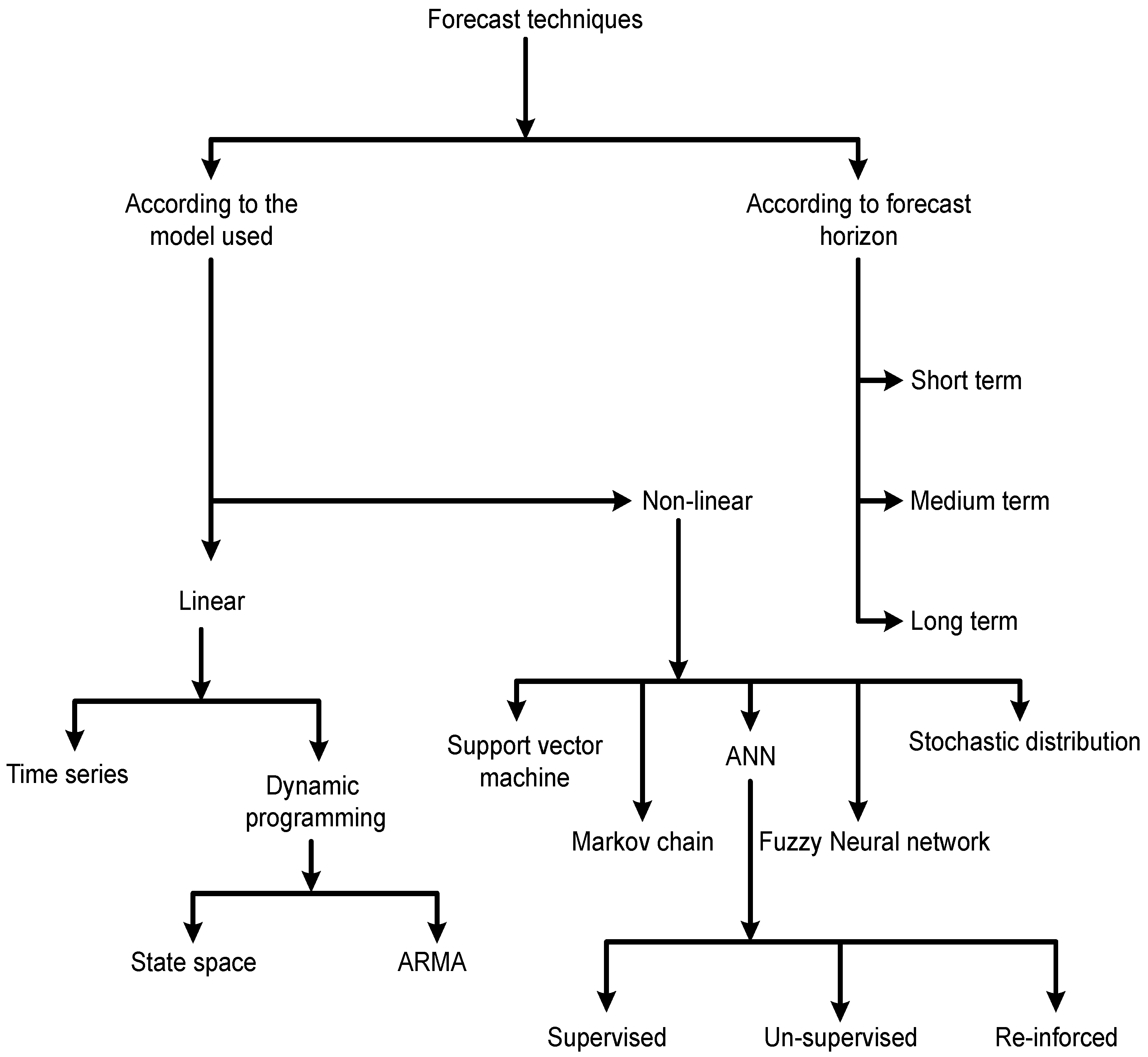
2.1. Linear Models

Linear models give continuous response which is a function or linear combination of one or more prediction variables. These models depend on the synthesis of all features of a problem that is more or less solved by complex equations. Examples of these models include spectral decomposition-based models, ordinary least square-based models, ARMA, etc. Since the prediction of demand is complex due non-linearities, the linear forecast models predict with high relative errors due to their inability to map the complex relationship between input and output. Thus, development of linear models is highly challenging. Furthermore, Hagan et al. [10] highlighted the relative limitation(s) of linear models as compared to non-linear models. Therefore, this research work is focused towards the discussion of non-linear models only.

2.2. Non-Linear Models

When the observational data is modeled by non-linear combination of one or more prediction variables, the model is said to be non-linear. To describe the relation between residual and periodical components, Bunn and Farmer [32] realize/conclude the ability of non-linear models to overcome the limitation(s) of linear models. In reference [9], the non-linear models are further categorized into five classes: (i) support vector machine-based models; (ii) Markov chain-based models; (iii) ANN-based models; (iv) fuzzy neural network-based models; and (v) stochastic distribution-based models. These models are discussed as follows.

(i) Support vector machine-based models: In reference [11], Niu et al. propose support vector machine and ant colony optimization-based load-forecasting technique for an SG. The authors use ant colony optimization technique for preprocessing of the input data. In this paper, system mining technique is used for feature selection. The selected features are fed into the forecaster which is a support vector machine-based predictor. Another important work has been presented by Li et al. in [12]. This varied version of the authors is least squares-based support vector machine. Similarly, reference [13] models the cyclic nature of demand by support vector machine-based linear regression. In conclusion, the support vector machine-based works are better in terms of accuracy; however, development of these models is highly challenging due to high complexity.

(ii) Markov chain-based models: Subject to robustness of DALF forecast strategy, authors in [14] propose a Markov chain-based strategy. This stochastic strategy aims to tackle load-time series fluctuations associated with energy consumption of users in a heterogeneous environment. The Markov chains are used to predict the future duty cycles of appliances. The technique is robust due to their memoryless nature (predicted pattern only depends on the current states; past states are not considered). In reference [15], Markov chain Monte Carlo method is used to model the switching pattern of household appliances. In simulations, they consider 100 households for one weak. However, this model limited in scope as it applies to situations in the Netherlands only. Another work in [16] proposes explicit duration hidden Markov model along with differential observation-based model to predict individual load of appliances. The authors collect the aggregated power signals by ordinary smart meters. The memoryless nature of Markov chains not only makes the DALF strategy robust but also relatively less complex in comparison to the aforementioned techniques. However, the memory less nature of Markov chains also has a drawback; less accuracy.

(iii) ANN-based models: ANNs learn from experience/training to predict future values while being fed with relevant input information. The advantages of these networks include but are not limited to self-organization, adaptive learning, fault tolerance, ease of integration with existing network/technology, and real time operation. The abilities to generalize and to capture non-linearity in complex environments make ANNs very attractive in problems of load forecasting. There are two basic architectures of ANN; feed forward and feedback. The former one carries information from input to output via hidden layer in forward direction only, i.e., the information of each layer is independent from that of the others. Feed forward ANNs are widely used for pattern recognition and forecasting problems. The later one carries information in both directions, forward and feedback, such that the information of each layer is dependent on that of the others. Feedback ANNs are appropriate for complex and time varying problems [33,34,35]. On the other hand, the learning modes of ANNs fall under three categories: supervised [36], unsupervised [37], and re-enforced [38]. In the first category, the ANN attempts to minimize minimum square error (MSE) for known target vector (i.e., the input/output vectors are specified). For a given input/output, error is calculated between output and the target values. This error is used to update the weights and biases of the ANN to minimize the MSE to a certain threshold. In the second category, the ANN does not need explicit target data. The system adjusts its output based on self-learning from different input patterns. In the third category, the connections between ANs are reinforced every time these are activated. Since this research work is limited in scope to supervised learning only, we discuss some of these latest/relevant works as follows.

In reference [27], authors present a hybrid technique subject to short-term price forecasting of SGs. This hybrid technique comprises two steps; feature selection and prediction. In the first step, a mutual information-based technique is implemented to remove redundancy and irrelevancy from the input load-time series. In the second step, ANN along with evolutionary algorithm is used to forecast the time series of the future load. In this process, the authors assume sigmoid activation function for artificial neurons (ANs), and Levenburg-Marquardt algorithm for training. In addition, the authors fine-tune some adjustable parameters during the first and second steps via an iterative search procedure which is part of their work. Subject to forecast accuracy, this technique is efficient as it embeds various techniques; however, the cost paid is high execution time. In reference [28], the authors investigate stochastic characteristics of SG’s load. More importantly, the authors present a bi-level DALF technique for SGs. In the first/lower level, ANN and evolutionary algorithm are implemented to forecast the future load/price curve. In the second/upper level, an EDE algorithm is implemented to further minimize the prediction errors. Effectiveness of this work is reflected via MATLAB simulations which demonstrate that the proposed strategy performs DALF in SGs with a reasonable accuracy by paying the cost of high execution time. The hybrid methodology in [39] completes the DALF task in four steps: (i) data selection; (ii) transformation; (iii) forecast; and (iv) error correction. In step one, some well-known techniques of data selection are used to minimize the high dimensionality curse of input load-time series characteristics. Step two deals wavelet transformation of the selected characteristics of input load-time series to enable redundancy and irrelevancy filter implementation. Followed by step three, which uses ANN and a training algorithm subject to DALF in SGs. More importantly, they choose sigmoid activation function for ANs due non-linear capturability. Finally, error correcting functions are used in step four to improve the proposed DALF methodology in terms of accuracy. In simulations, this methodology is tested against practical household load which demonstrates that this methodology is very good for improving the accuracy by paying the cost of high complexity. Another novel strategy is presented in [40] to predict the occurrence of price spikes in SGs. The proposed strategy uses wavelet transformation for input feature selection. An ANN is then used to predict future price spikes based on the training of the selected inputs.

(iv) Fuzzy neural network-based models: Doveh et al. [21] present fuzzy ANN-based model for load forecasting. In their work, the input variables are heterogeneous. They also model the seasonal effect via a fuzzy indicator. In reference [22], the authors present a self-adaptive load-forecasting model for SGs. To correlate demand profile information and the operational conditions, a knowledge-based feedback fuzzy system is proposed. For optimization of error, a multilayered perceptron ANN structure is used where training is done via back propagation method. Some other hybrid strategies such as [23,24] focus on fuzzy ANN as well. Wang [23] presents electric demand forecasting model using fuzzy ANN model, whereas, Che et al. [24] present an adaptive fuzzy combination model. Che et al. iteratively combine different subgroups while calculating fuzzy functions for all the subgroups. A few more works combining fuzzy ANN with other schemes are presented in [25,26]. Subject to fuzzy neural network controller design for improving prediction accuracy, membership functions to express the inference rules by linguistic terms need proper definitions. As fuzzy systems lack such formal definitions, optimization of these functions is thus a potential research area. However, the integration of optimization technique further complicates the overall methodology.

(v) Stochastic distribution-based models: The model in [17] predicts the power usage time series by using a probability-based approach. The model also configures household appliances between holidays and working days. A major assumption in this work is the gaussian distribution-based on-off cycles of household appliances, number of appliances, and power consumption pattern of appliances. In this work, not only a wide range of appliances is considered but also high flexibility degree of appliances is considered. However, absence of closed form solution makes the gaussian-based forecast strategy very complex. Moreover, these assumptions cannot be always true, thus, accuracy of the predicted load-time series is highly questionable. An improvement over [17] is presented in [18]. This research work uses $\frac{1}{2}$ regulizer to overcome the computational complexity of gaussian distribution-based DALF strategy in [17]. Moreover, the proposed DALF strategy can capture heteroscedasticity of load in a more efficient way as compared [17]. Simulations are conducted to prove that the proposed DALF strategy performs better than the existing one. To sum up, we conclude that [18] has overcome the complexity of [17] to some extent; however, the basic assumptions (gaussian distribution-based on-off cycles of household appliances, number of appliances, and power consumption pattern of appliances) still hold the bases and thus make the proposal highly questionable in terms of accuracy. A semi-parametric additive forecast model is presented in [19]. This work is based on point forecast and calculates the prediction intervals via a modified bootstrap algorithm. Similarly, another semi-parametric generalized additive load forecast model is presented in [20]. In terms of forecast horizon, the generalized additive forecast model is better than the non-generalized one due to its dual forecast capability; short-term and middle term. However, both the forecast models are not sufficient in terms of accuracy when compared to the ANN-based models. The overall classification hierarchy of forecast techniques is shown in Figure 2, and their summary is given in

Table 1. Performance analyses of the selected forecast classes.

Forecast Class	Accuracy	Execution Time	Convergence Rate	Remarks
Support vector machine-based models [11,12,13]	Moderate	High	Slow	These models achieve relatively moderate accuracy, however, at the cost of high execution time (slow convergence rate) due to high complexity.
Markov chain-based models [14,15,16]	Low	Low	Fast	Forecast accuracy of these models needs improvement.
ANN-based models [27,28,39,40]	Low to moderate	Low to high	Fast to slow	Hybrid ANN-based models improve the forecast accuracy of ANN-based models, but at the cost of high execution time (slow convergence rate).
Fuzzy ANN-based models [21,22,23,24,25,26]	Low to moderate	High	Slow	Execution time (convergence rate) need improvement.
Stochastic distribution-based models [17,18,19,20]	Low	High	Slow	Both forecast accuracy, and execution time (convergence rate) need improvement.

.

3. The Proposed Forecast Strategy

ANNs are widely used as forecasters because these networks can predict the non-linearities of SGs’ load with low convergence time. However, sometimes the achieved prediction accuracy is not up to the mark. Thus, leading to the adoption of optimization techniques that can significantly enhance the prediction accuracy of ANNs. However, the cost paid to achieve high accuracy is increased convergence time. Therefore, we aim towards the development of a new DALF strategy using the concept of hybrid integration subject to: (i) improvement of prediction accuracy; and (ii) reduction of convergence time.

Our proposed DALF strategy is implemented in three interconnected modules: (i) a pre-processing module; (ii) a forecast module; and (iii) an optimization module. Given the input data, the pre-processing module removes redundant and irrelevant samples from the input data. Using sigmoid activation function and MARA, the hybrid ANN-based forecast module predicts the DAL of an SG. Finally, the optimization module minimizes prediction errors to improve accuracy of the overall DALF strategy. Block diagram of the proposed model is shown in Figure 3. Detailed description of each module is as follows.

3.1. Pre-Processing Module

Since the ANN-based forecaster predicts load of the next day, the input data must be pre-processed subject to removal of redundant and irrelevant samples due to two reasons: (i) redundant features do not provide more information and thus unnecessarily increase the execution time during the training process (will be later discussed in the forecast module); and (ii) irrelevant features do not provide useful information and act as outliers. Detailed description of the pre-processor module is as follows.

As mentioned earlier, the data preparation module receives the input load-time series (historical). Suppose, following is the input load data:

$$P=\left[\begin{array}{ccccc}p(h_1,d_1)& p(h_2,d_1)& p(h_3,d_1)& \dots & p(h_m,d_1)\\ p(h_1,d_2)& p(h_2,d_2)& p(h_3,d_2)& \dots & p(h_m,d_2)\\ p(h_1,d_3)& p(h_2,d_3)& p(h_3,d_3)& \dots & p(h_m,d_3)\\ p(h_1,d_4)& p(h_2,d_4)& p(h_3,d_4)& \dots & p(h_m,d_4)\\ p(h_1,d_5)& p(h_2,d_5)& p(h_3,d_5)& \dots & p(h_m,d_5)\\ ⋮& ⋮& ⋮& \ddots & ⋮\\ p(h_1,d_n)& p(h_2,d_n)& p(h_3,d_n)& \dots & p(h_m,d_n)\end{array}\right]$$

(1)

where, $d_n$ is the nth day, $h_m$ is the mth hour of the day, and $p(h_m,d_n)$ is power usage value of the of the nth day at the mth hour. Similarly, we have input dew point temperature data in a matrix $T_{DP}$, input dry bulb temperature data in a matrix $T_{DB}$, and the input type of day (working day or holiday) data in a matrix $D_T$. Choosing n is totally dependent on the choice of designer. Greater value of n means that more historical lagged samples are available (fine tuning). This fine tuning however results in greater time during execution of the algorithm. Thus, there is a trade-off between convergence rate and accuracy. Before feeding the forecast/prediction module with P, the values of P are normalized. In this process, a local maximum value ‘$p_{max}^{c_i}$’ is computed in each column of P:

$$\begin{array}{c}\hfill p_{max}^{c_i}=max(p(h_i,d_1),p(h_i,d_2),p(h_i,d_3),\dots \\ \hfill ,p(h_i,d_n)),\forall i\in \{1,2,3,\dots ,m\}\end{array}$$

(2)

By local normalization we mean normalization of each P’s column by local maxima (one maximum in each column); results are saved in $P_{nrm}$ (range of $P_{nrm}$∈$[0,\dots ,1]$). Similarly, the matrices $T_{DP,nrm}$, $T_{DB,nrm}$ and $D_{T,nrm}$ are normalized forms of $T_{DP}$, $T_{DB}$ and $D_T$, respectively.

These input matrices $P_{nrm}$, $T_{DP,nrm}$, $T_{DB,nrm}$ and $D_{T,nrm}$ not only contain irrelevant features but also contain redundant features. To remove these two types of features, we use mutual information technique that is proposed in [27] and later used in [28] as well. According to this technique, the relative amount of mutual information between two quantities; input K and target G, is as follows:

$$MI(K,G)=\sum _i\sum _{j}p(K_i,G_j)lo{g}_2\left(\frac{p(K_i,G_j)}{p\left(K_i\right)p\left(K_i\right)}\right)$$

(3)

In reference (3), MI$(K,G)=0$ reflects that the input and target variables and independent, high value of MI$(K,G)$ reflects that there is a strong relation between K and G two and low value of $MI(K,G)$ reflects that there is loose relation between K and G.

By using (3), we calculate MI$(K,G)$ with the help of which two types of samples (redundant plus irrelevant) are discarded from the given input data matrices $P_{nrm}$, $T_{DP,nrm}$, $T_{DB,nrm}$ and $D_{T,nrm}$. According to [27,28], this MI technique achieves acceptable accuracy while not taking high time for execution.

Remark 1.

The data set used for training is historical, i.e., for tomorrow’s load forecast we need measured load values of previous days. Yes! The historical data was time dependent however with respect to the current day these values do not undergo any change. In other words, we deal with previously recorded data which means that the stationary assumption is not violated. Thus, the computation of MI is applicable here.

Remark 2.

The power consumption/demand of a user is different for days such as holidays or working days. It even shows variation for different hours such as on-peak and off-peak hours. To better explain our choice, let us consider the following example:

Considering matrix P in Equation (1), let $p(h_1,d_1)$ be the prediction variable. Then there are two possible cases for training:

(a) 

The ANN is trained by all elements of the matrix P except the first row.

(b) 

The ANN is trained only by the 1st column of the matrix P except $p(h_1,d_1)$.

The training samples in case (a) lead to greater prediction error due to the presence of outliers. Whereas, the training samples in case (b) lead to smaller prediction error because the outliers are removed.

Remark 3.

To improve accuracy of a forecast/prediction model, the samples used for training must be a-priori made relevant. Also, minimized number of samples will decrease algorithm’s execution time. Due to these two reasons, we prefer/chose local training for each hour. In our approach, the historical load values are locally normalized by local maxima. Then the normalized values are binary encoded with respect to local median. This encoding represents two classes of values: high and low. The classes are used for selecting features only, i.e., the mutual information is easily calculated for binary variables. This selection reduces the computational complexity of the mutual information-based feature selection strategy. Once we get rid of redundant and irrelevant samples are removed from the data set, the actual values against the binary encoded values are used for training and optimization in the rest of the modules to prevent information loss. Thus, we have used a compromising approach between computational complexity and information loss.

Remark 4.

Feature selection is done at beginning, and the selected features are then used for training during the operational life of the technique. From simulations, we conclude the following:

(i) 

If the data set size is small (≤1 month), feature selection has no significant impact on the computational complexity of the overall strategy.

(ii) 

If the data set size is moderate (≥1 month and ≤3 months), feature selection somehow affects the computational complexity of the overall strategy.

(iii) 

If the data set size is large (≥3 months), feature selection has a significant impact on the computational complexity of the overall strategy.

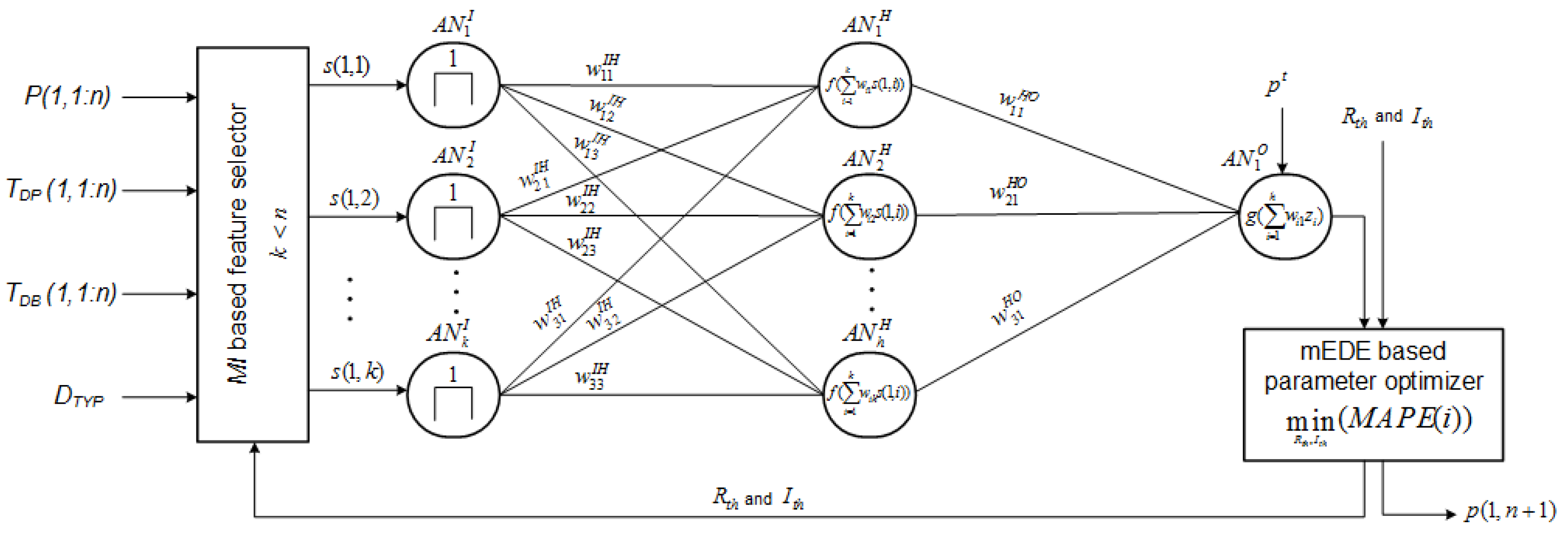
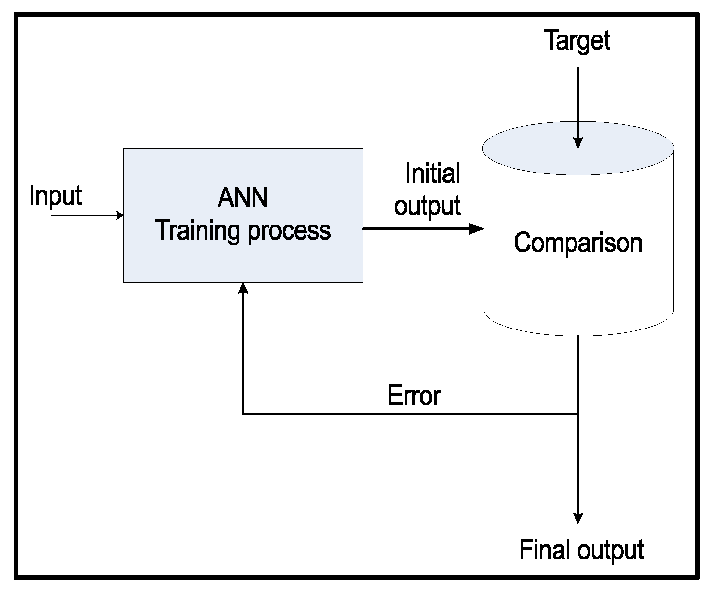
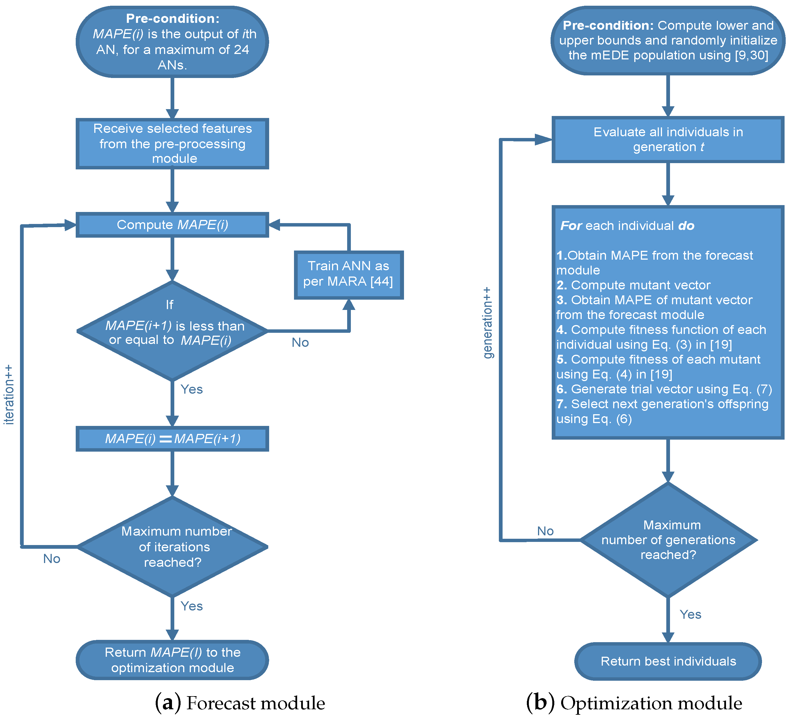
3.2. Forecast Module

From the works discussed in Section 2, it is concluded that any DALF strategy must ensure non-linear prediction capability. Therefore, we choose ANNs because these can capture the highly volatile characteristics of load-time series with reasonable accuracy.

For DALF, two strategies are used; direct forecasting and iterative forecasting [28]. However, it is discussed in [41] that the first strategy may introduce significant round off errors and the second one introduces large forecast errors. To overcome these imperfections, reference [28] has introduced the idea of cascaded strategy. Thus, our proposed forecast module implements the cascaded strategy. Our forecast module consists of an ANN; 24 consecutive cascaded forecasters such that each one of the 24 forecasters has an output for forecasting an hour’s load of the upcoming day. It is worth mentioning that the 24 h’ forecasters/predictors are modeled explicitly instead of a single implicit/complex one. These 24 one hour ahead forecasters allow improvement in terms of accuracy [28]. The cascaded ANN forecast structure is a combination of direct and iterative structures such that load of each hour of the next day is directly predicted and each forecaster yields exactly one output.

In the forecast module, each forecaster is an AN that implements sigmoid function for activation. We have chosen sigmoid activation function because for enabling ANs in terms of capturing the highly volatile (non-linear) SG’s time variant load characteristics. To update the weights during training process of the ANN, different algorithms have been used previously. For example, reference [42] include Gradient Descent Back Propagation algorithm. Similarly, references [27,28] suggest Levenberg-Marquardt algorithm as it can train the ANN 1–100 times faster than the Gradient Descent Back Propagation algorithm. We use multivariate auto regressive algorithm (MARA) [43] because it can train the ANN faster than Levenberg-Marquardt algorithm and Gradient Descent Back Propagation algorithm [42]. According to Kolmogrov theorem, if the ANN is provided with proper number of ANs then it can solve a problem by adopting one hidden layer. Thus, we have considered one hidden layer in the cascaded ANN structure of all 24 ANs. From the selected features $S_f(.)$ of the pre-processing module, the forecast module constructs training and validation samples, $S_T=S_f(i,j)$ and $S_V=S_f(1,j)$, respectively (where $i\in [2,m]$ and $j\in [1,n]$). These samples illustrate that the training of ANN by all the candidate inputs except the last/final one. The set of last samples of historical load-time series is used for validation purpose. In fact, the validation set is a part of the training load set constructed from it the training. Thus, the validation set becomes unseen for ANN. To make the validation error as a true representative of the forecast error, validation set needs to be as close to the forecast horizon as possible. While forecasting tomorrow’s load we choose one day backward samples due to two reasons: (i) daily periodicity; and (ii) short-run trend [44]. Thus, each of the 24 ANs is trained as per multi-variate MARA using the aforementioned training and validation sets. Further details of the training process to update the weights can be found in [43] and pictorial view of the learning process is shown in Figure 4.

For a set of finite input-target pairs, once the weights are adaptively adjusted as per MARA [43], the forecast module returns the forecast error signal; mean absolute percentage error ‘$MAPE\left(i\right)=\frac{1}{m}{\sum }_{j=1}^m\frac{|p^a(i,j)-p^f(i,j)|}{p^a(i,j)}$’, to the optimization module. Where $p^a(i,j)$ is the actual load value and $p^f(i,j)$ is the forecasted load value. Stepwise operations of the proposed forecast module are shown in Figure 5a.

3.3. Optimization Module

Based on the nature of the overall forecast strategy, the basic objective of optimization module is to minimize the forecast error, $E_F(.)$,

$$\underset{I_{th},R_{th}}{\mathit{minimize}}\mathrm{MAPE}\left(i\right)$$

(4)

where $i\in [1,m]$, $I_{th}$ and $R_{th}$ represent thresholds for irrelevancy and redundancy, respectively. Optimization module gives $I_{th}$’s and $R_{th}$’s optimized values to the $\mathrm{MI}$-based feature selection module which uses these threshold values for feature selection. For this purpose, various choices are available such as linear programming, non-linear programming, quadratic programming, convex optimization, heuristic optimization, etc. However, the first one is not applicable here because the problem is highly non-linear. The non-linear problem can be converted into a linear one; however, the overall process would become very complex. The second one is applicable here and gives accurate results by paying execution time’s cost. Similarly, the third and fourth ones suffer from slow convergence time. It is worth mentioning here that optimization does not imply exact reachability to optimum set of solutions, rather, near optimal solution(s) is(are) obtained. To sum up, heuristic optimization techniques are preferred in these situations because these provide near optimal solution(s) in relatively less execution time.

DE is one of the heuristic optimization techniques proposed in [45] and its enhanced version is used for forecast error minimization in [28]. In this paper, we modify the EDE algorithm for the sake accuracy improvement. Thus, in the upcoming paragraphs, detailed discussion is presented.

According to [28], in generation t, the jth trial vector y for ith individual is given as:

$$\begin{array}{c}\hfill y_{i,j}^{{}^{\prime }t}=\left\{\begin{array}{cc}{u}_{i,j}^t\hfill & \mathrm{if}rnd\left(j\right)\le F{F}_N\left(U_i^t\right)\hfill \\ x_{i,j}^t\hfill & \mathrm{if}rnd\left(j\right)>F{F}_N\left(U_i^t\right)\hfill \end{array}\right.\end{array}$$

(5)

where, $x_{i,j}^t$ and $u_{i,j}^t$ are the corresponding parent and mutant vectors, respectively. In (5), $F{F}_N(.)$ denotes the fitness function ($0<F{F}_N(.)<1$) and $Rand\left(j\right)\in [0,1]$ is a random number complying to uniform distribution. Between $X_i^t$ and $Y_i^t$, the corresponding offspring of the next generation $X_i^{(t+1)}$ is selected as follows:

$$\begin{array}{c}\hfill y_{i,j}^t=\left\{\begin{array}{cc}{y}_{i,j}^{{}^{\prime }t}\hfill & \mathrm{if}\mathrm{MAPE}\left(y_i^{{}^{\prime }t}\right)\le E_F\left(x_i^t\right)\hfill \\ x_{i,j}^t\hfill & \mathrm{otherwise}\hfill \end{array}\right.\end{array}$$

(6)

where, $\mathrm{MAPE}(.)$ is the objective function. From (5) and (6), it is clear that offspring selection depends on the trial vector which in turn depends on the random number and the fitness function. From this discussion, we conclude that the selected offspring is not the fittest. To make the fittest one, our approach eliminates the chances of offspring selection under the influence of random number, i.e., we modify (5) as follows:

$$\begin{array}{c}\hfill y_{i,j}^{{}^{\prime }t}=\left\{\begin{array}{cc}{u}_{i,j}^t\hfill & \mathrm{if}\frac{X_i^t}{X_{i_{max}}^t}<F{F}_N\left(U_i^t\right)\hfill \\ x_{i,j}^t\hfill & \mathrm{if}\frac{X_i^t}{X_{i_{max}}^t}\ge F{F}_N\left(U_i^t\right)\hfill \end{array}\right.\end{array}$$

(7)

From (7), it is clear that the trial vector no longer depends on the random number instead its dependence in now totally on the mutant vector which in turn depends on the parent vector. Offspring selection by this method will ensure selection of the fittest ones subject to accuracy improvement. Stepwise operations of the optimization module are shown in Figure 5b.

4. Simulation Results

For evaluation of our proposed model, we conduct simulations. For simulations, we have used MATLAB installed on Intel(R) Core(TM) i3-2370M CPU @ 2.4GHz and 2GB RAM with Windows 7. The proposed MI+ANN+mEDE-based forecast model is compared with two existing DALF models: MI+ANN forecast [27], and bi-level forecast [28]. For simulation purpose, traces of real time data for DAYTOWN and EKPC (the two USA grids) are taken from PJM electricity market. This data is freely available at [46]. We have used January–December 2014 load values for training the ANN, and January–December 2015 data for testing the ANN. Following are the simulation parameters that are used in our experiments (refer to

Table 2. Parameters used in simulations.

Parameter	Value
Forecasters	24
Hidden layers	1
Maximum iterations	100
Neurons (in the hidden layer)	5
Bias	0
Initial weights	$0.1$
Momentum	0
Load data (historical)	1 year
Maximum generations	100

). Justification of these parameters can be found in [27,28,42,43]. The newly proposed MI+ANN+mEDE model is tested against the two existing models in terms of three performance metrics: (i) accuracy; and (ii) execution time or convergence rate.

• Accuracy:$Accuracy(.)=100-\mathrm{MAPE}(.)$. We have measured this metric in %.
• Variance:$Var\left(i\right)=\frac{1}{m}{\sum }_{j=1}^m|p^f(i,j)-\overline{p^a(i,j)}|$. Where $\overline{p^a(i,j)}$ is the mean value of $p^a(i,j)$. Monthly variance is calculated by using the same formula while considering the calculated daily variances.
• Execution time: During simulations, the time taken by the system to completely execute a given forecast strategy. The strategy for which execution time is small converges more quickly and vice versa. In simulations, we have measured execution time in seconds.

Referring to Figure 6a–f and

Table 3. EKPC: Results for January 2015.

Day	Forecast Model
	MI+ANN		Bi-Level		MI+ANN+mEDE
	MAPE	Variance	MAPE	Variance	MAPE	Variance
1	3.99	1.89	2.40	1.50	1.04	1.12
2	3.42	1.78	1.97	1.46	1.32	0.97
3	4.10	2.08	2.61	1.26	1.15	1.09
4	3.67	1.91	2.13	1.41	1.44	0.96
5	3.79	1.70	1.97	1.37	1.16	1.05
6	3.62	1.88	2.43	1.48	1.29	0.97
7	3.93	1.73	2.62	1.39	1.40	1.11
8	3.97	1.94	1.92	1.28	1.19	1.03
9	3.54	2.04	2.18	1.42	1.39	0.90
10	3.46	1.79	2.21	1.36	1.10	1.03
11	4.05	1.72	1.85	1.39	1.25	1.05
12	4.21	1.84	1.97	1.29	1.29	0.90
13	3.89	2.00	1.94	1.33	1.07	1.03
14	3.62	1.75	1.84	1.46	1.36	1.10
15	3.79	1.99	2.11	1.26	1.14	0.93
16	3.47	1.81	2.44	1.38	1.36	1.07
17	4.24	2.10	2.26	1.26	1.20	1.04
18	4.20	1.74	2.61	1.41	1.23	1.08
19	3.86	1.97	2.44	1.46	1.07	0.96
20	3.61	1.80	2.52	1.42	1.18	0.98
21	3.82	1.95	2.29	1.48	1.36	1.12
22	3.77	2.03	2.62	1.45	1.42	0.99
23	4.23	1.86	2.53	1.51	1.34	1.01
24	3.94	1.77	2.38	1.29	1.11	0.92
25	3.44	1.73	2.20	1.47	1.32	1.14
26	3.56	1.94	2.23	1.34	1.10	0.97
27	3.81	1.78	2.29	1.40	1.24	1.11
28	3.39	1.82	1.94	1.29	1.39	1.03
29	4.19	2.05	2.43	1.32	1.08	0.98
30	3.52	1.77	1.98	1.42	1.12	1.06
31	4.01	1.99	1.82	1.42	1.33	0.99
Average	3.81	1.84	2.23	1.38	1.24	1.03

,

Table 4. EKPC: Results for 2015.

Month	Forecast Model
	MI+ANN		Bi-Level		MI+ANN+mEDE
	MAPE	Variance	MAPE	Variance	MAPE	Variance
January	3.81	1.84	2.23	1.38	1.24	1.03
February	3.85	1.75	2.15	1.44	1.20	0.99
March	4.76	1.90	2.26	1.39	1.26	1.05
April	3.84	1.76	2.19	1.41	1.29	1.00
May	3.80	1.71	1.20	1.47	1.23	1.02
June	3.73	1.73	2.16	1.35	1.21	1.01
July	3.72	1.81	2.29	1.40	1.24	1.07
August	3.84	1.70	1.28	1.40	1.25	1.03
September	3.82	2.90	2.22	1.33	1.20	0.99
October	3.82	1.88	2.15	1.36	1.30	1.01
November	4.77	1.75	1.17	1.48	1.22	1.06
December	4.80	1.82	1.27	1.32	1.27	1.02
Average	3.79	1.80	2.13	1.39	1.24	1.01

,

Table 5. DAYTOWN: Results for January 2015.

Day	Forecast Model
	MI+ANN		Bi-Level		MI+ANN+mEDE
	MAPE	Variance	MAPE	Variance	MAPE	Variance
1	3.72	1.70	2.59	1.36	1.20	1.02
2	3.60	1.86	2.38	1.30	1.31	1.10
3	3.54	1.90	2.20	1.51	1.35	0.97
4	3.81	1.88	1.77	1.27	1.25	0.95
5	3.78	1.92	2.57	1.41	1.32	1.07
6	4.07	1.83	2.65	1.33	1.21	0.96
7	3.88	1.79	2.58	1.43	1.35	1.11
8	3.62	1.81	2.25	1.28	1.22	1.01
9	4.30	1.88	2.25	1.50	1.15	0.90
10	3.71	1.93	2.43	1.44	1.27	1.03
11	3.59	1.77	2.27	1.30	1.34	1.12
12	3.82	1.74	2.34	1.37	1.24	0.95
13	3.77	1.84	2.50	1.25	1.29	1.06
14	4.15	1.83	2.64	1.31	1.16	1.13
15	3.69	1.91	1.88	1.40	1.28	0.93
16	3.87	1.89	2.47	1.52	1.30	1.12
17	4.27	2.76	2.60	1.33	1.29	1.10
18	3.64	1.78	2.15	1.42	1.31	1.00
19	4.18	1.84	1.86	1.40	1.21	1.12
20	3.75	1.99	2.31	1.28	1.19	0.99
21	3.58	1.97	2.05	1.39	1.18	1.05
22	3.83	2.72	2.70	1.30	1.32	0.98
23	4.88	1.99	2.60	1.38	1.37	1.09
24	3.73	1.88	2.44	1.29	1.18	1.12
25	4.21	2.01	1.91	1.47	1.33	0.92
26	3.59	1.76	1.79	1.32	1.21	1.04
27	3.80	1.96	2.20	1.37	1.24	1.10
28	3.66	1.89	1.97	1.27	1.22	1.03
29	4.25	1.81	2.33	1.49	1.15	0.98
30	3.51	1.92	1.90	1.24	1.36	1.03
31	4.03	1.95	1.88	1.43	1.20	1.06
Average	3.86	1.92	2.27	1.36	1.25	1.03

and

Table 6. DAYTOWN: Results for 2015.

Month	Forecast Model
	MI+ANN		Bi-Level		MI+ANN+mEDE
	MAPE	Variance	MAPE	Variance	MAPE	Variance
January	3.86	1.92	3.27	1.36	1.25	1.03
February	3.85	1.71	2.30	1.47	1.20	0.99
March	3.80	1.75	2.20	1.44	1.22	1.05
April	3.71	1.79	2.24	1.38	1.27	1.06
May	3.79	1.87	2.28	1.40	1.22	1.02
June	3.72	1.85	2.13	1.30	1.24	1.07
July	3.76	1.76	2.22	1.36	1.28	0.99
August	3.87	1.76	2.18	1.43	1.26	1.08
September	3.70	2.70	2.29	1.38	1.23	1.02
October	3.77	1.88	2.17	1.36	1.21	1.09
November	3.83	1.83	2.27	1.50	1.27	1.00
December	3.80	1.81	2.25	1.33	1.21	1.01
Average	3.78	1.88	2.31	1.39	1.23	1.03

, which are graphical/tabular illustrations/representations of the proposed MI+ANN+mEDE-based forecast model versus the two existing DALF models: MI+ANN and bi-level. From Figure 6a,b, it is clear that the proposed MI+ANN+mEDE model effectively predicts/forecasts the future load of the two selected SGs. The ANN-based forecaster captures the non-linearities in the history load-time series. This non-linear prediction capability is not only due to sigmoid activation function but also due to the selected training algorithm; MARA. When we look at the hourly forecast results in Figure 6c,d, the % error of the MI+ANN-based forecast model is $3.8\%$ and $3.81\%$ for DAYTOWN and EKPC, respectively. The % error of the bi-level forecast model is $2.2\%$ and $2.23\%$ for DAYTOWN and EKPC, respectively. The % error of the proposed MI+ANN+mEDE-based forecast model is $1.24\%$ for both DAYTOWN and EKPC, respectively. Similarly, the daily forecast results of the two simulated models for January 2015 are shown in Table 3 and Table 5 for the two selected USA grids, respectively. From these results, it is clear that the existing MI+ANN-based forecast model predicts the future load with the highest % error and the highest variance. Also, the monthly forecast results of the three simulated models for January–December 2015 are shown in Table 4 and Table 6 for EKPC and DAYTOWN, respectively. From Table 4 and Table 6, it is evident that the proposed MI+ANN+mEDE model forecasts the future load with the least prediction error and the least variance as compared to the other two existing models. This result is obvious due to absence of optimization module in MI+ANN-based forecast model. To minimize this forecast error, the bi-level forecast model uses EDE algorithm. Subject to further minimization of the forecast error, we have integrated an mEDE optimization technique. Please note that mEDE is our modified version of existing EDE algorithm for down scaling forecast error. Results show that integration of mEDE algorithm yields fruitful results; the MI+ANN+mEDE-based DALF model is relatively more accurate than the other two existing DALF models. These figures show the positive impact of optimization module on the forecast error minimization between target curve and the forecast curve. It is obvious that the error curve decreases as the number of generations of the mEDE algorithm are increased. As the proposed MI+ANN+mEDE forecast model compares the forecast curve’s error (next generation) with the existing one (existing generation) and updates the weights if the forecast curve’s error is less than the existing one (survival of the fittest). Thus, as expected, the forecast error is significantly minimized as the forecast strategy is subjected to step ahead generations. However, during simulations, we observed that from 89th to 100th generation, the forecast error does not exhibit significant improvement. Therefore, the proposed and the existing forecast models are not subjected to further generations. There exists a possible trade-off between accuracy of a forecast strategy and its convergence rate (refer to Section 1, Section 2 and Section 3). This trade-off is shown in Figure 6c–f. From these figures, it is clear that the bi-level forecast model improves the accuracy of MI+ANN forecast model while paying cost in terms of relatively slow convergence rate. On the other hand, the newly proposed MI+ANN+mEDE model modifies the EDE algorithm to further improve the accuracy of the bi-level forecast model. More importantly, the MI+ANN+mEDE model improves the prediction accuracy by not paying surplus cost in terms of execution time. However, the execution time of our proposed forecast model is still greater than the MI+ANN forecast model due to integration of optimization module.

Figure 7 shows the impact of dataset size (number of training data samples) on error performance (see Figure 7a) and execution time (see Figure 7b) of the three selected models. By observing Figure 7a, an improvement of error performance for all the compared STLF models is evident when the number of lagged input samples increase from 30 to 120. This result follows Equation (1), i.e., the ANN is more finely tuned by increasing the value of n (30 to 120) which improves the forecast error performance. However, this improvement is not significant at much higher tuning when the number of training samples are increased from 60 to 120 (stability can be seen in the curves). On the other hand, Figure 7b shows the cost of high execution time paid by the fine tuning to achieve relative improvement in forecast accuracy. This is obvious because training of the ANN takes additional time when the number of training samples are increase. From Figure 7a,b, it is clear that the proposed modular model is more scalable (relatively higher degree of stability can be seen for MI+ANN+mEDE forecast) as compared to the other two models. The reasons for this higher scalability are: usage of selected features for training of the ANN, training the ANN via MARA algorithm with local normalization, and usage mEDE algorithm for error minimization.

Table 7. Comparison of training iterations (convergence) and regression analysis (accuracy).

Dataset	Forecast Model	Iterations	Training	Testing	Validation
DAYTOWN	MI+ANN	20	0.9626	0.9619	0.9556
	Bi-Level	94	0.9787	0.9799	0.9776
	MI+ANN+mEDE	95	0.9876	0.9890	0.9872
EKPC	MI+ANN	23	0.9622	0.9617	0.9551
	Bi-Level	95	0.9769	0.9783	0.9766
	MI+ANN+mEDE	96	0.9877	0.9892	0.9878

shows the relationship between MAPE and the number of iterations of the three compared STLF models when tested on DAYTOWN and EKPC datasets. The convergence characteristics (i.e., the number of iterations) indicate that the proposed MI+ANN+mEDE model and the bi-level model converge at an optimal value in almost the same number of iterations. On the other hand, the MI+ANN model takes only 20–23 iterations for converging into an optimal target value. This result is obvious due to the added computational burden in the bi-level and the MI+ANN+mEDE models (i.e., these models use the optimization module) which is not the case in MI+ANN model (i.e., this model does not use the optimization model). In other words, the MI+ANN model achieves its target of the required training, testing, and validation with the least number of iterations. However, this least computational burden is achieved by paying the high cost of forecast accuracy. In this regard, a regression analysis of the network was performed to evaluate confidence interval of the training, testing and validation performance of the compared forecast models, and the results are shown in Table 7. Clearly, the proposed MI+ANN+mEDE model achieves the highest confidence interval (i.e., 98%) as compared to bi-level (i.e., 97%) and MI+ANN (i.e., 96%) models. This means that only 2% of the estimated data is not statistically significant for the network in case of the proposed MI+ANN+mEDE model. As a result, the forecasted load demand of the proposed MI+ANN+mEDE model is rather closer to its actual value as compared to the other two models (see Figure 6a,b).

5. Conclusions and Future Work

In SGs, DALF is an essential task because its accuracy has a direct impact on the planning schedules of utilities that strongly affects the energy trade market. Moreover, high volatility in the history load curves makes DALF in SGs relatively more challenging when compared to load forecast for longer duration. Taking into account DALF influencing factors such as exogenous variables and meteorological variables, we have presented a hybrid ANN-based DALF model for SGs which is a multi-model forecasting ANN with a supervised architecture and MARA for training. The proposed model significantly reduced the execution time and enhanced the forecast accuracy by distinctly carrying local normalization and local training. Moreover, sigmoid activation function and MARA enable the forecast strategy to capture non-linearities in load-time series. Integration of optimization module (based on our proposed modifications) with the forecast strategy also improved the forecast accuracy. Tests are conducted on three USA grids: DAYTOWN, EKPC and FE. Results show that the proposed model achieves relatively better forecast accuracy ($98.76\%$) in comparison to an existing bi-level technique and an MI+ANN technique. Moreover, improvement in forecast accuracy is achieved while not paying the cost of slow convergence rate. Thus, the trade-off between convergence rate and forecast is not created. Finally, from application perspective, the proposed model can be used by utilities to launch better offers in the electricity market. This means that the utilities can save significant amount of money due to better adjustment of their generation and demand schedules simply because of high accuracy of the proposed model.

In future, we are interested in advanced signal processing techniques for feature selection and extraction purposes. Moreover, exploration of particle swarm optimization-based techniques and a complete forecast plus scheduling-based technique is also under consideration.

References

- Gelazanskas, L.; Gamage, K.A. Demand side management in smart grid: A review and proposals for future direction. Sustain. Cities Soc. 2014, 11, 22–30. [Google Scholar] [CrossRef]
- Yan, Y.; Qian, Y.; Sharif, H.; Tipper, D. A Survey on Smart Grid Communication Infrastructures: Motivations, Requirements and Challenges. IEEE Commun. Surv. Tutor. 2013, 15, 5–20. [Google Scholar] [CrossRef]
- National Institute of Standards and Technology. NIST Framework and Roadmap for Smart Grid Interoperability Standards. Release 1.0.; 2010. Available online: http://www.nist.gov/publicaffairs/releases/upload/smartgridinteroperabilityfinal.pdf (accessed on 10 November 2018 ).
- Leiva, J.; Palacios, A.; Aguado, J.A. Smart metering trends, implications and necessities: A policy review. Renew. Sustain. Energy Rev. 2016, 55, 227–233. [Google Scholar] [CrossRef]
- How Does Forecasting Enhance Smart Grid Benefits? SAS Institute Inc.: Cary, NC, USA, 2015; pp. 1–9.
- Hernandez, L.; Baladron, C.; Aguiar, J.M.; Carro, B.; Sanchez-Esguevillas, A.J.; Lloret, J.; Massana, J. A survey on electric power demand forecasting: Future trends in smart grids, microgrids and smart buildings. IEEE Commun. Surv. Tutor. 2014, 16, 1460–1495. [Google Scholar] [CrossRef]
- Vardakas, J.S.; Zorba, N.; Verikoukis, C.V. A Survey on Demand Response Programs in Smart Grids: Pricing Methods and Optimization Algorithms. IEEE Commun. Surv. Tutor. 2015, 17, 152–178. [Google Scholar] [CrossRef]
- Hippert, H.S.; Pedreira, C.E.; Souza, C.R. Neural Networks for Short-Term Load Forecasting: A review and Evaluation. IEEE Trans. Power Syst. 2001, 16, 44–51. [Google Scholar] [CrossRef]
- Raza, M.Q.; Khosravi, A. A review on artificial intelligence based load demand forecasting techniques for smart grid and buildings. Renew. Sustain. Energy Rev. 2015, 50, 1352–1372. [Google Scholar] [CrossRef]
- Hagan, M.T.; Behr, S.M. The Time Series Approach to Short Term Load Forecasting. IEEE Trans. Power Syst. 1987, 2, 785–791. [Google Scholar] [CrossRef]
- Niu, D.; Wang, Y.; Wu, D. Power load forecasting using support vector machine and ant colony optimization. Exp. Syst. Appl. 2010, 37, 2531–2539. [Google Scholar] [CrossRef]
- Li, H.; Guo, S.; Zhao, H.; Su, C.; Wang, B. Annual Electric Load Forecasting by a Least Squares Support Vector Machine with a Fruit Fly Optimization Algorithm. Energies 2012, 5, 4430–4445. [Google Scholar] [CrossRef]
- Aung, Z.; Toukhy, M.; Williams, J.R.; S’anchez, A.; Herrero, S. Towards Accurate Electricity Load Forecasting in Smart Grids. In Proceedings of the Fourth International Conference on Advances in Databases, Knowledge, and Data Applications, Athens, Greece, 2–6 June 2012; pp. 51–57. [Google Scholar]
- Meidani, H.; Ghanem, R. Multiscale Markov models with random transitions for energy demand management. Energy Build. 2013, 61, 267–274. [Google Scholar] [CrossRef]
- Nijhuis, M.; Gibescu, M.; Cobben, J.F. Bottom-up Markov Chain Monte Carlo approach for scenario based residential load modelling with publicly available data. Energy Build. 2016, 112, 121–129. [Google Scholar] [CrossRef]
- Guo, Z.; Wang, Z.J.; Kashani, A. Home appliance load modeling from aggregated smart meter data. IEEE Trans. Power Syst. 2015, 30, 254–262. [Google Scholar] [CrossRef]
- Gruber, J.K.; Prodanovic, M. Residential energy load profile generation using a probabilistic approach. In Proceedings of the IEEE UKSim-AMSS 6th European Modelling Symposium, Valetta, Malta, 14–16 November 2012; pp. 317–322. [Google Scholar]
- Kou, P.; Gao, F. A sparse heteroscedastic model for the probabilistic load forecasting in energy-intensive enterprises. Electr. Power Energy Syst. 2014, 55, 144–154. [Google Scholar] [CrossRef]
- Fan, S.; Hyndman, R.J. Short-Term Load Forecasting Based on a Semi-Parametric Additive Model. IEEE Trans. Power Syst. 2012, 27, 134–141. [Google Scholar] [CrossRef]
- Goude, Y.; Nedellec, R.; Kong, N. Local Short and Middle Term Electricity Load Forecasting with Semi-Parametric Additive Models. IEEE Trans. Power Syst. 2014, 5, 440–446. [Google Scholar] [CrossRef]
- Doveh, E.; Feigin, P.; Greig, D.; Hyams, L. Experience with FNN Models for Medium Term Power Demand Predictions. IEEE Trans. Power Syst. 1999, 14, 538–546. [Google Scholar] [CrossRef]
- Mahmoud, T.S.; Habibi, D.; Hassan, M.Y.; Bass, O. Modelling self-optimised short term load forecasting for medium voltage loads using tunning fuzzy systems and Artificial Neural Networks. Energy Convers. Manag. 2015, 106, 1396–1408. [Google Scholar] [CrossRef]
- Wang, Z.Y. Development Case-based Reasoning System for Shortterm Load Forecasting. In Proceedings of the IEEE Russia Power Engineering Society General Meeting, Montreal, QC, Canada, 18–22 June 2006; pp. 1–6. [Google Scholar]
- Che, J.; Wang, J.; Wang, G. An adaptive fuzzy combination model based on self-organizing map and support vector regression for electric load forecasting. Energy 2012, 37, 657–664. [Google Scholar] [CrossRef]
- Nadimi, V.; Azadeh, A.; Pazhoheshfar, P.; Saberi, M. An Adaptive-Network-Based Fuzzy Inference System for Long-Term Electric Consumption Forecasting (2008–2015): A Case Study of the Group of Seven (G7) Industrialized Nations: USA, Canada, Germany, United Kingdom, Japan, France and Italy. In Proceedings of the Fourth UKSim European Symposium on Computer Modeling and Simulation, Pisa, Italy, 17–19 November 2010; pp. 301–305. [Google Scholar]
- Lou, C.W.; Dong, M.C. Modeling data uncertainty on electric load forecasting based on Type-2 fuzzy logic set theory. Eng. Appl. Artif. Intell. 2012, 25, 1567–1576. [Google Scholar] [CrossRef]
- Amjaday, N.; Keynia, F. Day-Ahead Price Forecasting of Electricity Markets by Mutual Information Technique and Cascaded Neuro-Evolutionary Algorithm. IEEE Trans. Power Syst. 2009, 24, 306–318. [Google Scholar] [CrossRef]
- Amjady, N.; Keynia, F.; Zareipour, H. Short-Term Load Forecast of Microgrids by a New Bilevel Prediction Strategy. IEEE Trans. Smart Grid 2014, 1, 286–294. [Google Scholar] [CrossRef]
- Liu, N.; Tang, Q.; Zhang, J.; Fan, W.; Liu, J. A Hybrid Forecasting Model with Parameter Optimization for Short-term Load Forecasting of Micro-grids. Appl. Energy 2014, 129, 336–345. [Google Scholar] [CrossRef]
- Ahmad, A.; Javaid, N.; Alrajeh, N.; Khan, Z.A.; Qasim, U.; Khan, A. A modified feature selection and artificial neural network-based day-ahead load forecasting model for a smart grid. Appl. Sci. 2015, 5, 1756–1772. [Google Scholar] [CrossRef]
- Ahmad, A.; Javaid, N.; Guizani, M.; Alrajeh, N.; Khan, Z.A. An accurate and fast converging short-term load forecasting model for industrial applications in a smart grid. IEEE Trans. Ind. Inform. 2017, 13, 2587–2596. [Google Scholar] [CrossRef]
- Bunn, D.W.; Farmer, E.D. Comparative Models for Electrical Load Forecasting; Wiley: New York, NY, USA, 1985; pp. 13–30. [Google Scholar]
- Ahmad, I.; Abdullah, A.B.; Alghamdi, A.S. Application of artificial neural network in detection of probing attacks. IEEE Sympos. Ind. Electron. Appl. 2009, 57–62. [Google Scholar]
- Malki, H.A.; Karayiannis, N.B.; Balasubramanian, M. Short term electric power load forecasting using feedforward neural networks. Exp. Syst. 2004, 21, 157–167. [Google Scholar] [CrossRef]
- Hahn, H.; Meyer-Nieberg, S.; Pickl, S. Electric load forecasting methods: Tools for decision making. Eur. J. Oper. Res. 2009, 199, 902–907. [Google Scholar] [CrossRef]
- Amakali, S. Development of Models for Short-Term Load Forecasting Using Artficial Neural Networks. Master’s Thesis, Cape Peninsula University of Technology, Cape Town, South Africa, 2008. [Google Scholar]
- Valova, I.; Szer, D.; Gueorguieva, N.; Buer, A. A parallel growing architecture for self-organizing maps with unsupervised learning. Neurocomputing 2005, 68, 177–195. [Google Scholar] [CrossRef]
- Anderson, J.; Silverstein, J.; Ritz, S.; Jones, R. Distinctive features, categorical perception and probability learning: Some applications on a neural model. Psychol. Rev. 1977, 84, 413–451. [Google Scholar] [CrossRef]
- Yang, H.T.; Liao, J.T.; Lin, C.I. A Load Forecasting Method for HEMS Applications. In Proceedings of the 2013 IEEE Grenoble Conference, Grenoble, France, 16–20 June 2013; pp. 1–6. [Google Scholar]
- Amjady, N.; Keynia, F. Electricity market price spike analysis by a hybrid data model and feature selection technique. Electr. Power Syst. Res. 2010, 80, 318–327. [Google Scholar] [CrossRef]
- Amjady, N.; Keynia, F. Short-term load forecasting of power systems by combination of wavelet transform and neuro-evolutionary algorithm. J. Energy 2009, 34, 46–57. [Google Scholar] [CrossRef]
- Engelbrecht, A.P. Computational Intelligence: An Introduction, 2nd ed.; John Wiley & Sons: New York, NY, USA, 2007. [Google Scholar]
- Anderson, C.W.; Stolz, E.A.; Shamsunder, S. Multivariate autoregressive models for classification of spontaneous electroencephalographic signals during mental tasks. IEEE Trans. Biomed. Eng. 1998, 45, 277–286. [Google Scholar] [CrossRef] [PubMed]
- Lasseter, R.H.; Piagi, P. Microgrid: A conceptual solution. In Proceedings of the IEEE International Conference on Power Electronics Specialists, Aachen, Germany, 20–25 June 2004; pp. 4285–4290. [Google Scholar]
- Storn, R.; Price, K. Differential evolution—A simple and efficient heuristic for global optimization over continuous spaces. J. Glob. Optim. 2009, 11, 341–359. [Google Scholar] [CrossRef]
- PJM Electricity Market. Available online: www.pjm.com (accessed on 1 February 2015).