Research on Gas Concentration Prediction Models Based on LSTM Multidimensional Time Series

Abstract

Effective prediction of gas concentrations and reasonable development of corresponding safety measures have important guiding significance for improving coal mine safety management. In order to improve the accuracy of gas concentration prediction and enhance the applicability of the model, this paper proposes a long short-term memory (LSTM) cyclic neural network prediction method based on actual coal mine production monitoring data to select gas concentration time series with larger samples and longer time spans, including model structural design, model training, model prediction, and model optimization to implement the prediction algorithm. By using the minimum objective function as the optimization goal, the Adam optimization algorithm is used to continuously update the weight of the neural network, and the network layer and batch size are tuned to select the optimal one. The number of layers and batch size are used as parameters of the coal mine gas concentration prediction model. Finally, the optimized LSTM prediction model is called to predict the gas concentration in the next time period. The experiment proves the following: The LSTM gas concentration prediction model uses large data volume sample prediction, more accurate than the bidirectional recurrent neural network (BidirectionRNN) model and the gated recurrent unit (GRU) model. The average mean square error of the prediction model can be reduced to 0.003 and the predicted mean square error can be reduced to 0.015, which has higher reliability in gas concentration time series prediction. The prediction error range is 0.0005–0.04, which has better robustness in gas concentration time series prediction. When predicting the trend of gas concentration time series, the gas concentration at the time inflection point can be better predicted and the mean square error at the inflection point can be reduced to 0.014, which has higher applicability in gas concentration time series prediction.

1. Introduction

China is a large coal consuming and producing country. Gas emissions from coal seams increase sharply during the coal mining process; gas overruns and coal and gas outbursts are frequent; and it has become a challenging topic for safe coal mine production. The key to preventing gas hazards is to effectively predict gas concentration and formulate effective extraction schemes. A lot of research has been done by domestic and foreign experts on the issue of gas concentration prediction. Fu’s team has done a lot of such research, and proposed the gas concentration of hybrid kernel least squares support vector machine based on phase space reconstruction theory and adaptive chaos particle swarm optimization theory [1,2,3,4]. In addition, scholars such as Wu used support vector machine (SVM) and the differential evolution (DE) algorithm to establish a prediction model, and based on the Markov chain, the residual correction predicted the gas concentration change trend, compared with the direct SVM prediction of the granular data [5]. Others have used neural networks to do more in-depth research. Liu proposed a prediction method combining genetic algorithm (GA) with back propagation (BP) neural network [6]. Guo proposed a dynamic prediction method based on time series for gas concentration [7]. Zhang proposed a dynamic nerve network gas concentration real-time prediction model for improved prediction accuracy of gas concentration and less running time [8]. The above method greatly improved the accuracy and reliability of gas concentration prediction, but the research data sample is small and has certain limitations, and it is difficult to adapt to more varied gas concentration sequences.

Long short-term memory (LSTM) is a time-recurrent neural network suitable for processing and predicting data with gaps and delays in a time series. Based on complex historical fault data, Wang proposed a fault time series prediction method based on a long short-term memory-cycle neural network. The multigrid parameter optimization algorithm was used to verify the LSTM prediction model in fault time. There is strong applicability in sequence analysis [9,10,11]. Based on the time series of factors affecting the operating state of the transformer, Dai used the fuzzy comprehensive evaluation idea to evaluate the operating state of the power transformer and establish prediction of the operating state of the power transformer based on LSTM [12]. Li proposed a long short-term memory-cycle neural network prediction model by analyzing the correlation between electricity price and load time series and using an adaptive evidence-based algorithm for deep learning [13,14,15]. Wang constructed a short-term traffic flow prediction model for LSTM–recurrent neural network (RNN) for traffic flow time series and achieved the prediction effect with layer-by-layer construction and fine-tuning [16,17,18,19]. Based on historical landslide time series, Yang proposed a dynamic prediction model of landslide displacement based on time series and LSTM. Combined with actual case verification, the prediction accuracy could be improved [20,21,22]. Relevant research at home and abroad shows that LSTM is suitable for processing sample data related to time series. Combined with the characteristics of gas concentration data, this paper proposes a gas concentration prediction model based on LSTM that can effectively predict the gas concentration in the next time period and provide a strong basis for formulating a reasonable gas drainage plan, thus improving coal mine safety management.

2. Materials and Methods

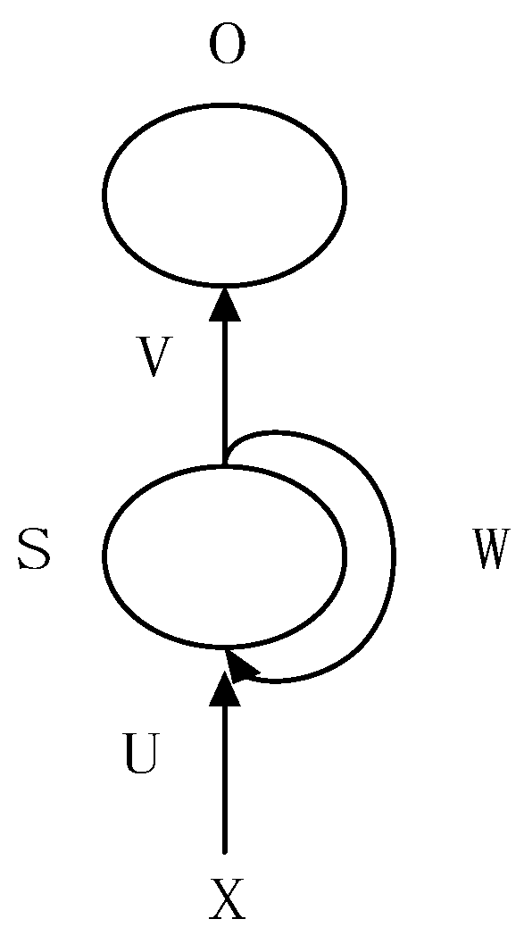
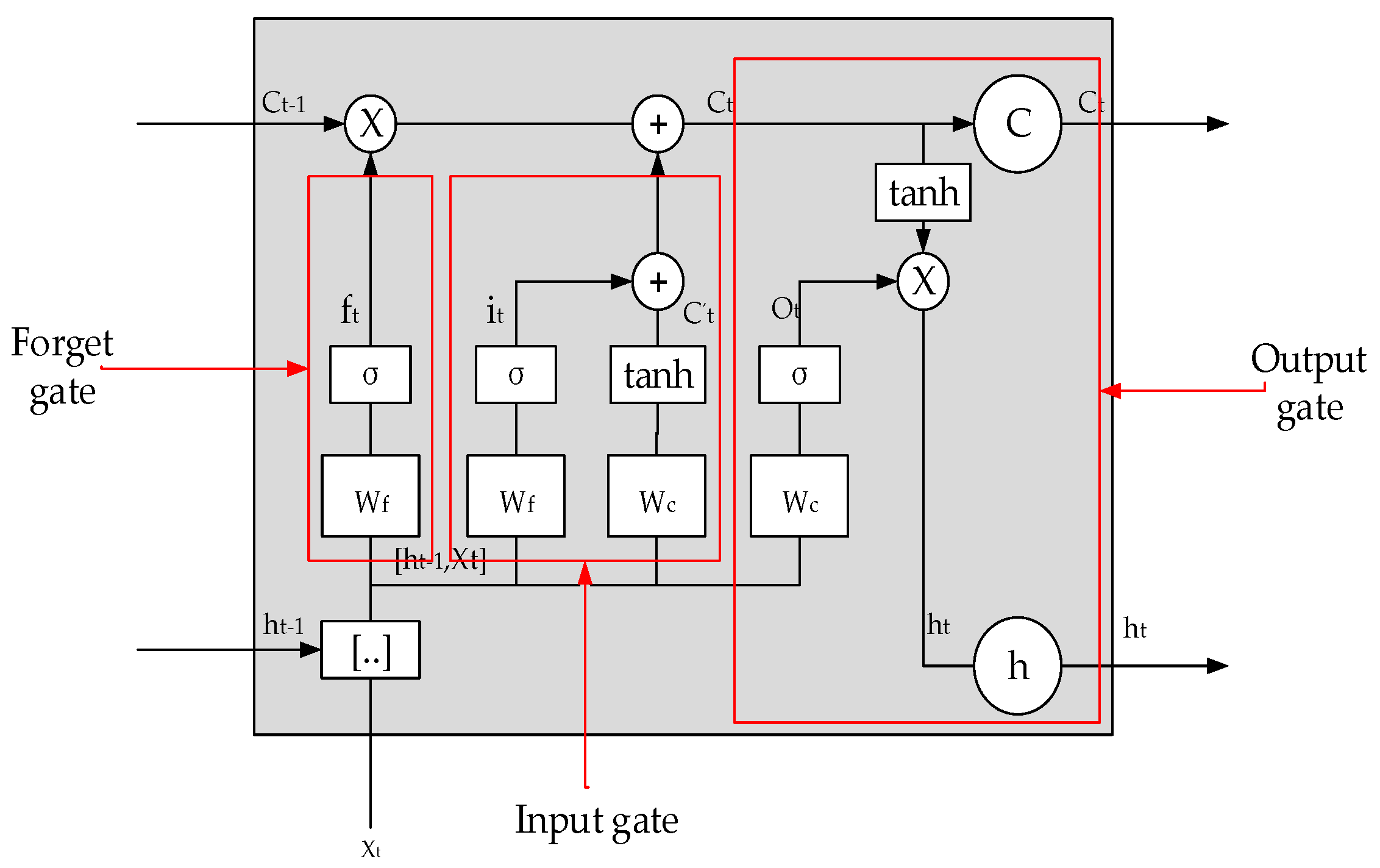
2.1. Deep Learning Model and Parameter Optimization Algorithm

This section briefly introduces the LSTM model, the Adam parameter optimization algorithm, and the related recurrent neural network (RNN) model. The traditional neural network model is from the input layer to the hidden layer to the output layer. The layers are fully connected and the nodes between each layer are disconnected. Therefore, ordinary neural networks have certain limitations in solving time series problems. The recurrent neural network compensates for the shortcomings of traditional neural networks. Its structure is shown in Figure 1, where X indicates the value of the input layer, S represents the value of the hidden layer, U is the weight matrix of the input layer to the hidden layer, O represents the value of the output layer, V is the weight matrix of the hidden layer to the output layer, and W is the last value of the hidden layer as the input of this time. The weight of t, t − 1 is time. Its running formula is:

$$\{\begin{array}{c}Q=g(V{S}_t)\\ S_t=f(U{X}_t+W{S}_{t-1})\end{array}$$

(1)

Although the RNN can effectively process nonlinear time series, it cannot handle time series with excessive delay due to gradient disappearance and gradient explosion. The LSTM is an improved cyclic neural network that solves the problem that the RNN cannot handle, i.e., long-distance dependencies. Figure 2 is a schematic structural view of the LSTM, where f_t, i_t, C_t, and O_t are the forget gate, the input gate, the output gate, and the timing of the output gate, respectively, and W, b, and tanh are the corresponding weights, deviations, and excitation functions, respectively. The forget gate determines how much of the unit state C_t−1 at the previous moment is retained at the current time C_t; the input gate determines how much the input X_t of the network is saved to the unit state C_t at the current moment and how much output gate control unit state C_t is output to the LSTM. The current output value is h_t. Its calculation formula is shown by Equations (2)–(4). The forget gate f_t is Equation (2), the input gate i_t is Equation (3), and the output gate O_t is Equation (4):

$$f_t=\delta (w_f·\left[h_{t-1},x_t\right]+b_f)$$

(2)

$$\{\begin{array}{c}{i}_t=\delta (w_i·\left[h_{t-1},x_t\right]+b_i)\\ C^{\prime }=\tanh (w_c·[h_{t-1},x_t]+b_c)\\ C_t=f_t·C_{t-1}+i_t·C_t^{\prime }\end{array}$$

(3)

$$\{\begin{array}{c}{O}_t=\delta (w_o·[h_{t-1},x_t]+b_o)\\ h_t=O_t·\tanh (C_t)\end{array}$$

(4)

A more popular concept at present is that circulating neural networks are gated recurrent units (GRUs) and bidirectional cyclic neural networks (BidirectionRNNs). A GRU is a light version of LSTM that has an update gate and a reset gate. The update gate is used to update information, and the reset gate is used to determine the output information. A BidirectionRNN is really just 2 independent RNNs put together.

Adaptive moment estimation (Adam) [23] is an optimization algorithm based on gradient. The method is simple, efficient, and has less memory usage. It is suitable for nonstationary objective functions. Hyperparameters have intuitive interpretations and do not require complex tuning procedures. Its update mechanism is as follows: deviation correction is Equation (5) and parameter change is Equation (7):

$$\{\begin{array}{c}m\_t=\beta \_1·m\_(t-1)+(1-\beta \_1)·g\_t\\ v\_t=\beta \_2·v\_(t-1)+(1-\beta \_2)·g\_t^{\wedge }2\end{array}$$

(5)

$$\{\begin{array}{c}{m}^{\prime }\_t=m\_t/(1-\beta \_1^{\wedge }t)\\ v^{\prime }\_t=v\_t/(1-\beta \_2^{\wedge }t)\end{array}$$

(6)

$$\theta \_t=\theta \_(t-1)-\alpha ·m^{\prime }\_t/(\sqrt{(v^{\prime }\_t)+\epsilon })$$

(7)

where β_1 = 0.9, β_2 = 0.99, ε = 1 × 10⁻⁸; the initial value of m_t and v_t is 0.

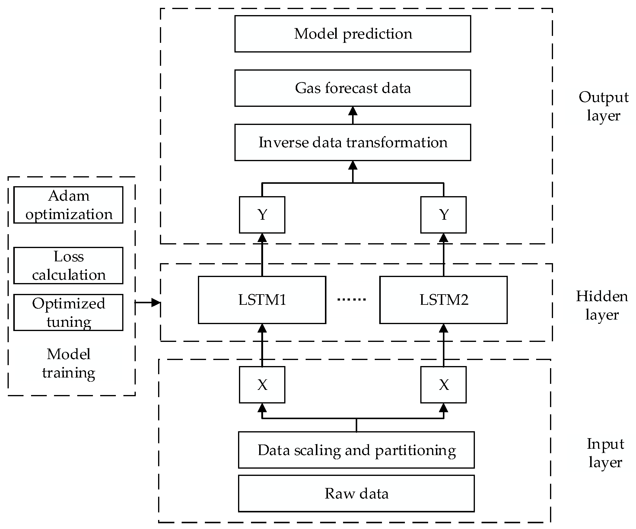
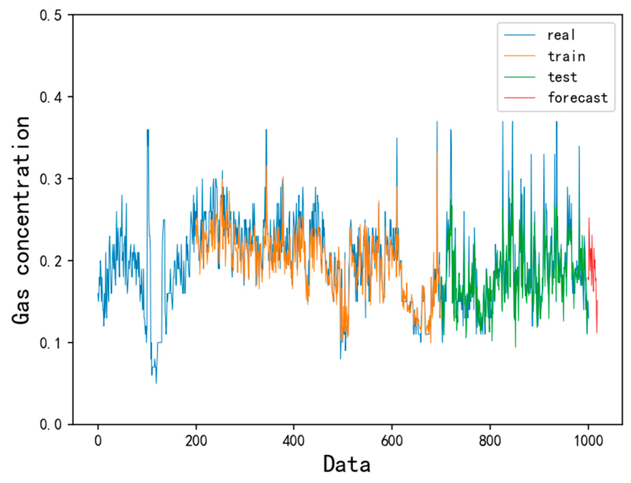
2.2. Construction of Predictive Model

The model can be divided into three parts: input layer, hidden layer, and output layer. The input layer is mainly used for preprocessing and dataset division of the original data. The hidden layer is trained based on the training set. Through the Adam optimizer, introduced in the previous section, the parameters are optimized, and the model is optimized with the minimum loss value as the measurement principle; the output layer predicts the data according to the model learned in the hidden layer and performs data restoration for scaling of the previous data preprocessing. The LSTM prediction model framework is shown in Figure 3.

The research object through model training is the hidden layer. The original input data in the input layer can be represented as D, and the original data is divided into training set T_r, test set T_e, and lookback, which is the previous time step used as an input variable to predict the next period. The training set T_r is normalized and scaled between 0 and 1 using the MinMaxScaler normalization formula. The scaled training set is T_rs. The MinMaxScaler formula is:

$$X\_std=(X-X.min(axis=0))/(X.max(axis=0)-X.min(axis=0))$$

(8)

$$X\_scaled=X\_std·(\mathit{max}-\mathit{min})+\mathit{min}$$

(9)

where X_std will be normalized to [0,1], X.min(axis = 0) indicates the column minimum, Max represents the parameter of the MinMaxScaler, and min represents the feature range parameter, which is the size range of the final result. The preprocessed training set X is defined as an input of the hidden layer, and its operation in the hidden layer of LSTM is as shown in Equations (2)–(4), and the output result is Y = LSTM(h_t).

The prediction is performed by using the trained LSTM network, where the prediction result training set is Tr_forecast’, the test set is Te_forecast’, and the next time is forecast_predict’. The preprocessed data are restored using scaler.inverse_transform, and the restored data are Tr_forecast, Te_forecast, and forecast_predict. Finally, the accuracy and fit of the model are determined by comparing Tr_forecast’ with Tr_forecast, Te_forecast’, and Te_forecast.

Because the setting of batch size determines the association information between time series data available to the LSTM, the number of network layers affects the learning ability, training time, and test time of the model; therefore, mean square error and fitting are used in training the LSTM model. The effect and running time are used as the criteria for evaluating the model. The Adam optimizer is used to optimize the weight of the LSTM structural unit, and the optimal parameter combination is obtained by continuously optimizing the batch size parameter of the network layer. For the time series of the same distribution characteristics, different activation functions have different effects, because the data used in this paper do not involve negative numbers, and the Relu activation function is used to improve the computing power and Dropout is added to prevent overfitting. Finally, the optimal LSTM prediction model is obtained.

3. Experiment and Results

This experiment mainly includes data selection and processing, prediction model adjustment, and optimization model comparison. In order to ensure the reliability and applicability of the model, we selected the monitoring data of the goaf from 1 January to 1 March 2017 at the Tingnan coal mine as the experimental sample. The data include four input variables: gas concentration, temperature, flow, and negative pressure, totaling 1100 pieces of data.

The computer configuration used in this experiment was as follows: Windows 10 64-bit operating system, AMD A6-6310 processor, 1.8 GHz frequency, 4 GB memory, Python 3.6 development language, and PyCharm Community Edition 2018.2.3 integrated development environment. The LSTM model used in the development of the program was derived from the Keras 2.1.5 package.

First, data was divided into a test set, a training set, a backtracking set, and a verification set, with the training set used for model training, the test set used to test the model learning effect, and the backtrack set used as an input variable to predict the next time period. For time series, the verification set was used to test the prediction data, then the data was cleaned, missing data was complemented by the near mean, abnormal data was deleted, and data whose format content did not conform to the specification was modified. Finally, the data included the characteristics of different dimension eigenvalues and target eigenvalue changes. The data was normalized by the MinMaxScaler method in Section 2.1 and scaled to [0,1] to facilitate calculation and improve predictive accuracy. The raw and processed data are shown in Figure 4 and Figure 5, respectively.

This paper mainly evaluates the performance of the model from 3 aspects: accuracy, fitting effect, and running time. Mean square error (MSE) was used as the evaluation index of model accuracy. The formula is:

$$MSE=\frac{1}{n}{\displaystyle {\sum }_{i=1}^n{(f_i-y_i)}^2}$$

(10)

where f_i, y_i are the predicted value and true value, respectively. The test results and real results of each optimization model were compared to evaluate the fitting effect of the model. The running time of each optimization model during the training test was counted to evaluate the computational efficiency of the model.

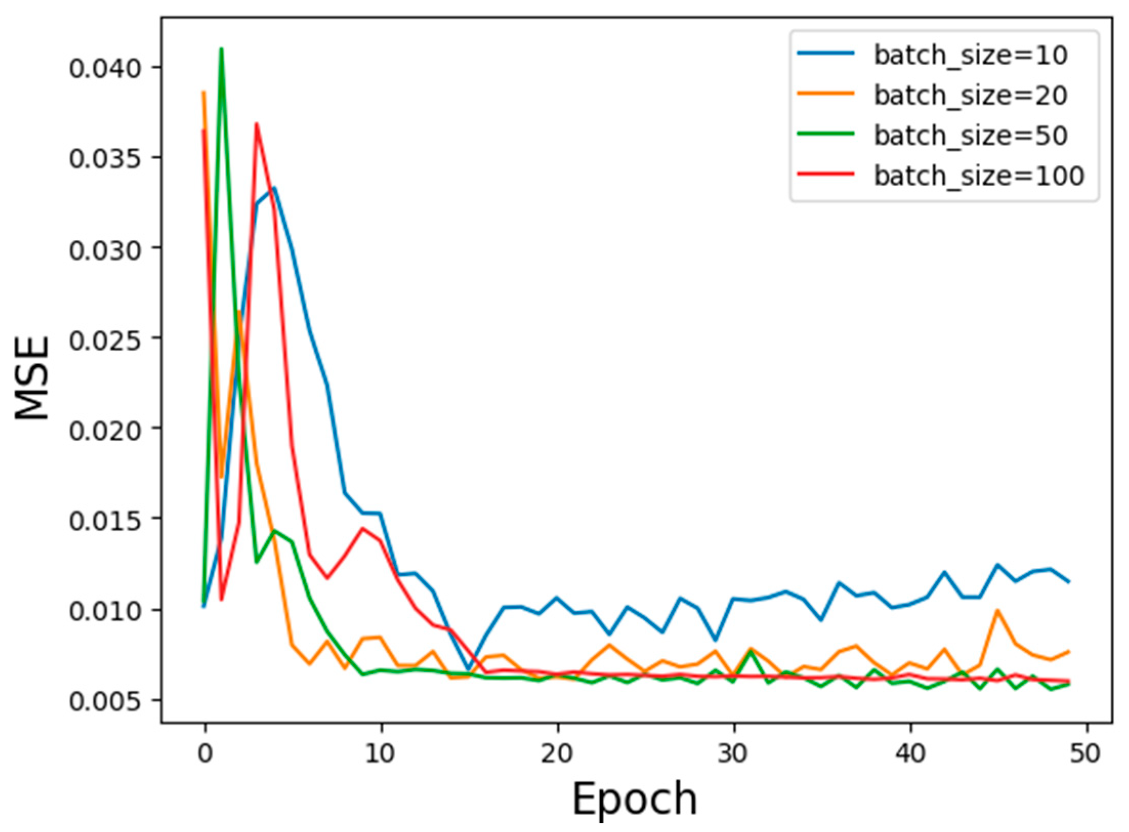
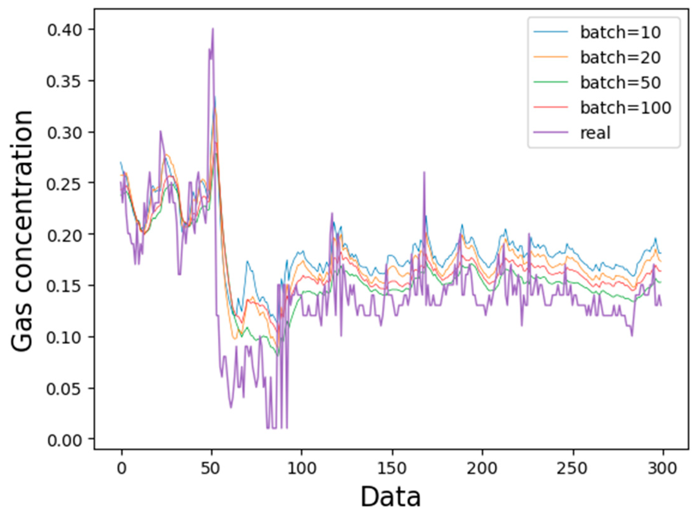
3.1. Optimization of Batch Size

Batch size [24] represents the length of the gas sequence that LSTM can utilize. It is a reaction of the data association length. To study the effect of batch size on the model, we set the number of LSTM network layers to 2 and the number of neurons to 64. Batch size was 10, 20, 50, and 100 performances, and the experimental results are shown in Figure 6 and Figure 7 and

Table 1. Batch size prediction results.

LSTM = 2 Layers; Neurons = 64
Batch	Operation Time	Mean Square Error
10	8 min	0.010897
20	5 min	0.009293
50	3 min	0.008331
100	2 min	0.009689

.

Figure 6 shows that when the batch size is 50 and 100, the loss value is about the same, which is obviously better than the loss value when the batch size is 10 and 20. When the batch size is 50, the prediction fit is the best. From Table 1, the batch size is 50, although the running time is not the shortest, but its MSE is the smallest. As the batch size increases, the prediction ability of the gas concentration prediction model improves. However, when the batch size is increased to a certain extent, although the running time is shortened, the prediction accuracy of the model does not improve; on the contrary, the fitting effect of the prediction result is degraded.

Taking into account prediction accuracy, running time, fitting effect, and other factors of the model, when the batch size is 50, the prediction effect of the model is the best, the running time is about 3 min, and the error can be reduced to 0.008.

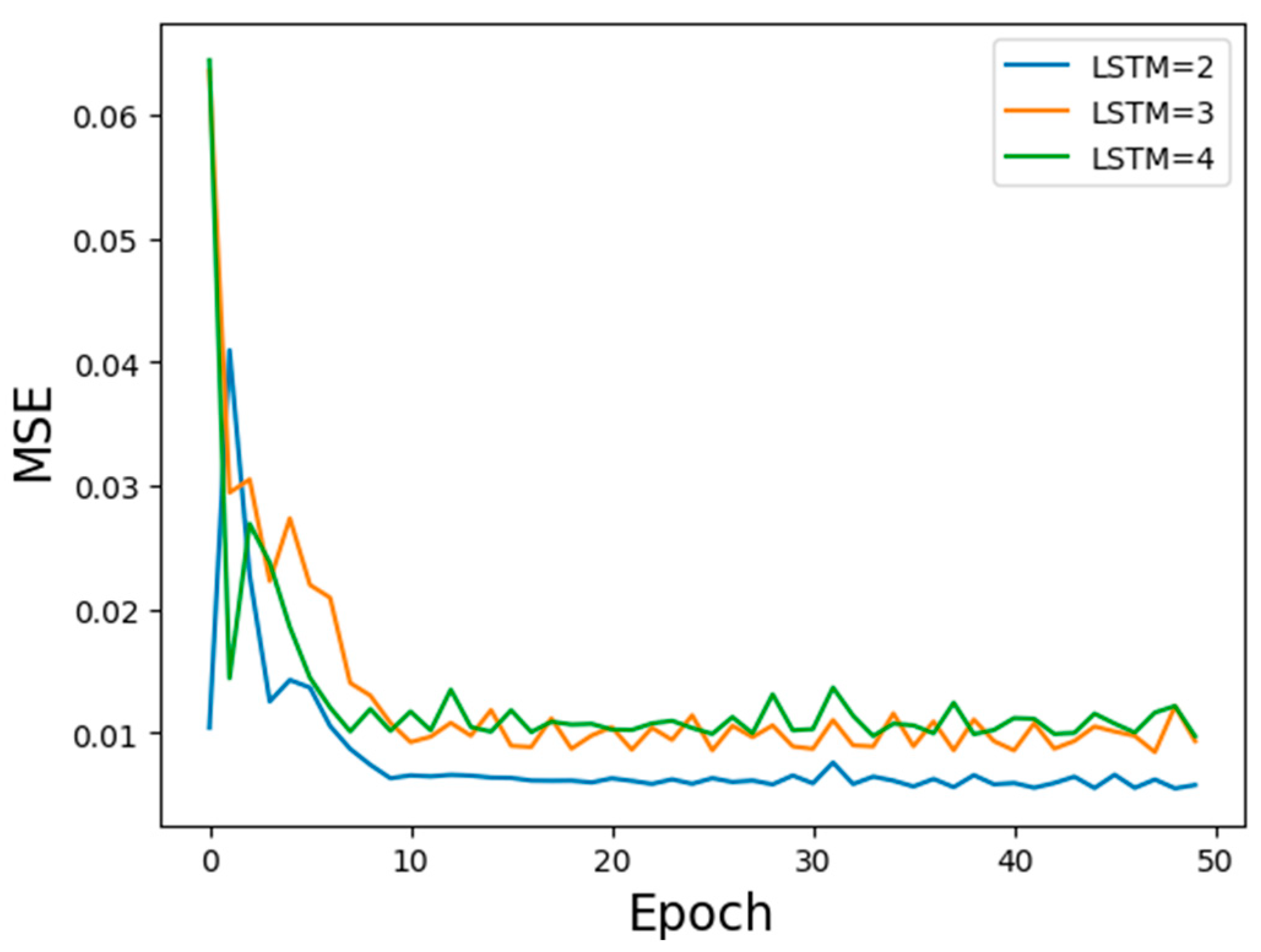
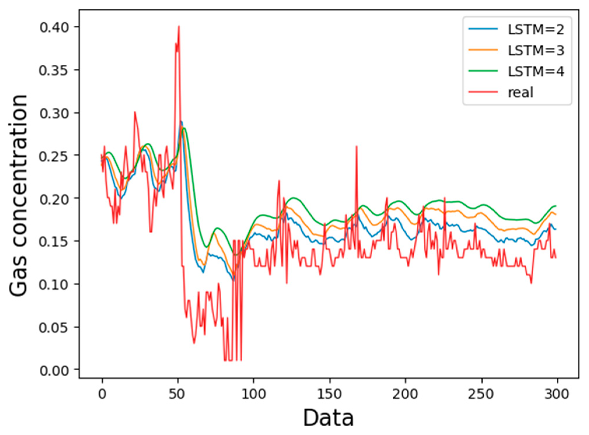
3.2. Optimization of Network Layer Number

The number of network layers will affect the learning ability, training time, and test time of the model. In theory, the deeper the LSTM layer, the stronger the learning ability. However, the deeper the model, the higher the complexity of the model, the more difficult it is to converge, and the more difficult and time consuming is the training. This paper compares the effects of LSTM with 2, 3, and layers, as shown in Figure 8 and Figure 9 and

Table 2. LSTM layer prediction results.

Batch Size = 50; Neurons = 64
LSTM Layers	Time	Mean Square Error
2	3 min	0.008331
3	6 min	0.012725
4	10 min	0.0155

.

Figure 6 shows that the loss value of two LSTM layers is significantly lower than that of three or four LSTM layers; the prediction results of the three layers in Figure 7 are slightly higher than the actual value, but the prediction with 2 LSTM layers has a result closer to the true data value. Figure 2 shows that the LSTM with two layers had the shortest time and least square error value. As the number of LSTM layers increases, the learning ability of the model is continuously enhanced, but the accuracy of prediction declines and the corresponding running time increases. Considering the accuracy, fitting effect, and running time of the model, the prediction effect of the 2-layer LSTM model is optimal.

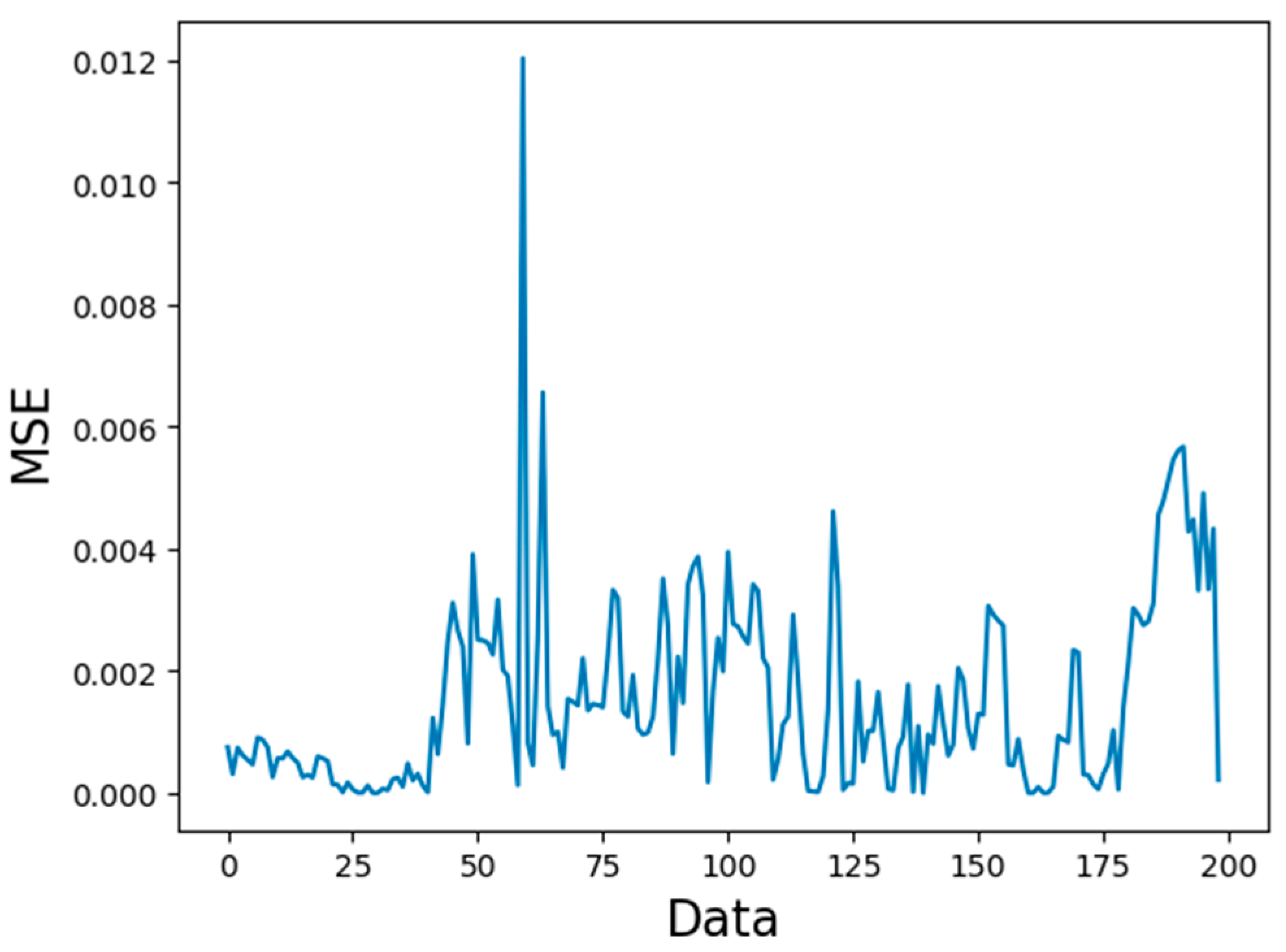
3.3. Comparison of Predicted Length

The key to the model is prediction. Therefore, predicting the next time period was studied in depth. The predicted length of the model is closely related to the selected batch size. The predicted timestep length is equivalent to the batch size. According to the previous experimental data, we chose the optimal batch size to be 50. We compared the prediction results with the timesteps of 1–4, as shown in Figure 10 and Figure 11 and

Table 3. Predicted length results.

Timestep	Mean Square Error	Maximum Error
1 (50)	0.000713	0.003381
2 (100)	0.001551	0.011366
3 (150)	0.001862	0.011355
4 (200)	0.001549	0.012031

.

When the predicted length timestep is 1, the loss value is at least 0.0005, and the prediction effect of the error variation region is good (Figure 10). With increased prediction length, the loss grows rapidly, and especially the individual gas concentration protrusion point prediction deviation is large. When the timestep is 1, the prediction model can better fit the law of gas concentration change. With increased prediction length, the fitting effect no longer meets the actual requirements and the inflection point appears as severe hysteresis at some time; the detailed prediction of the length error comparison is 4. When the timestep is 1, the maximum error is 0.003, which is in line with coal mine safety requirements. Considering that the accuracy of the prediction of gas concentration in actual production is high, the prediction effect is best when the timestep is 1.

The setting of the batch size determines the amount of related information between the time series data that the LSTM can utilize; the number of network layers affects the learning ability, training time, and test time of the model, and the multi-input variable information fusion can improve the performance of the model. In this paper, a batch size of 50, two LSTM network layers, and a 50-unit prediction length are the optimal parameters of the LSTM gas prediction model. After training, the model can better learn variations of gas concentration, especially at the inflection point of gas concentration change, which can show the superiority of the prediction model.

4. Discussion

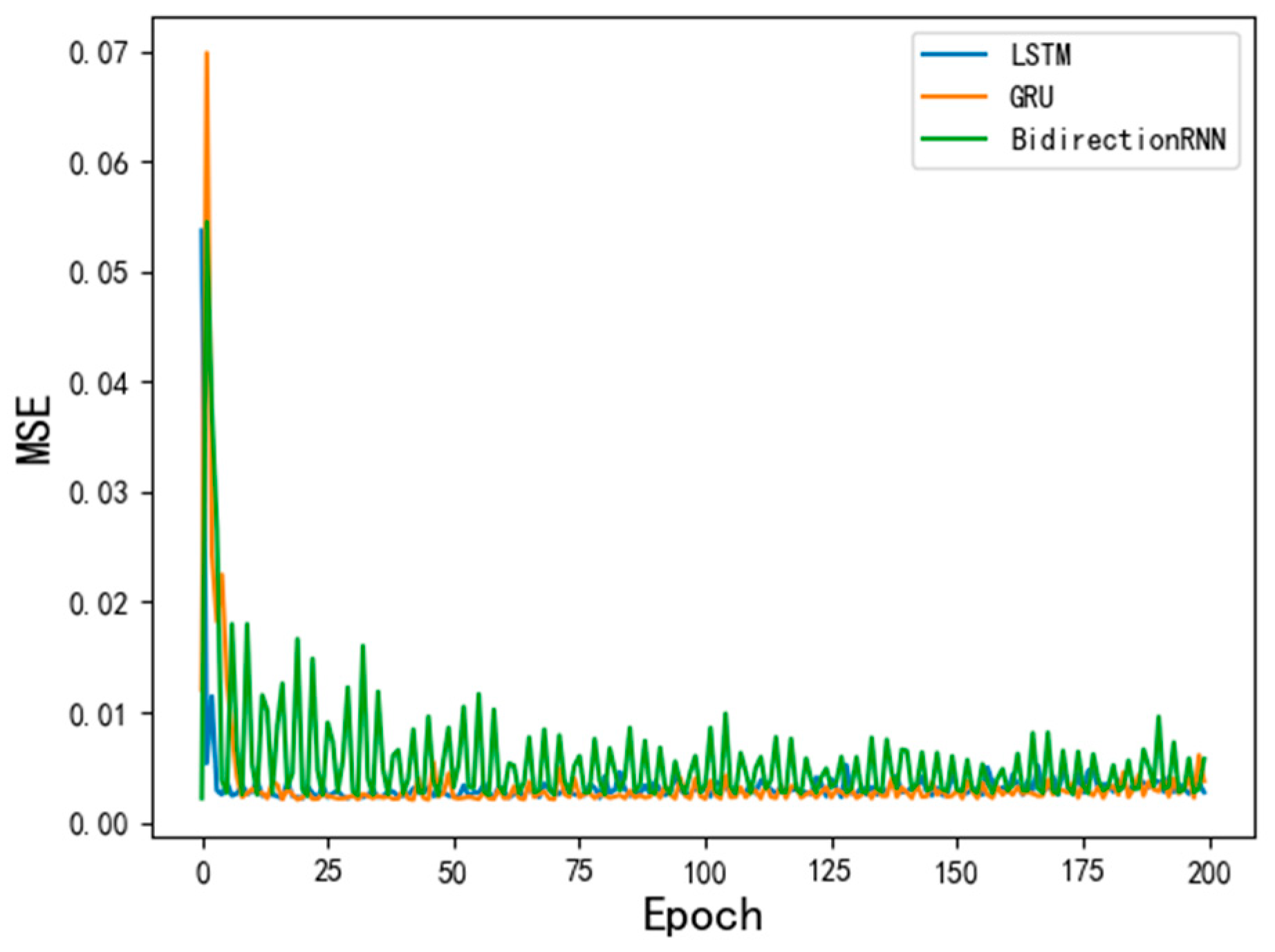
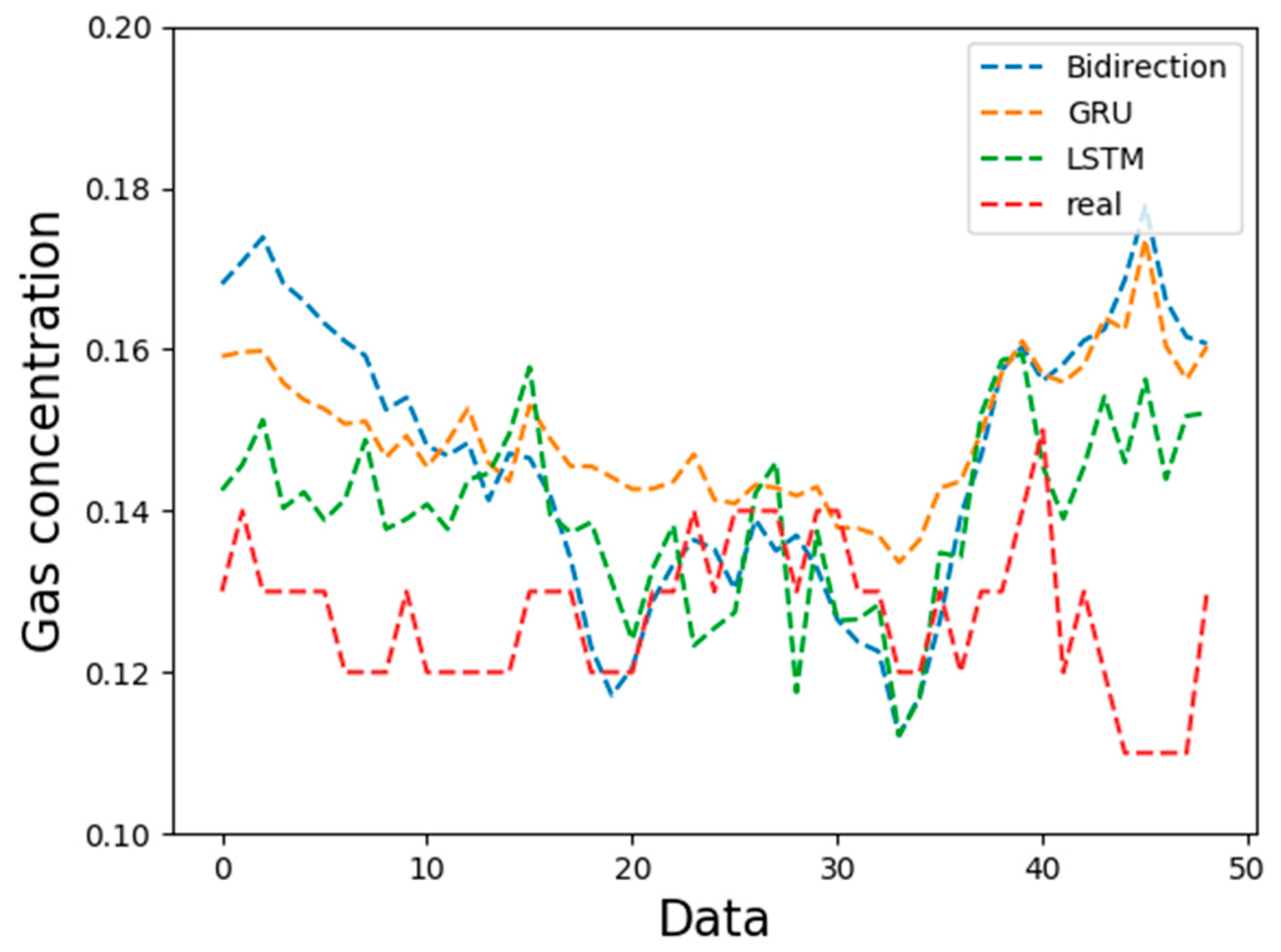
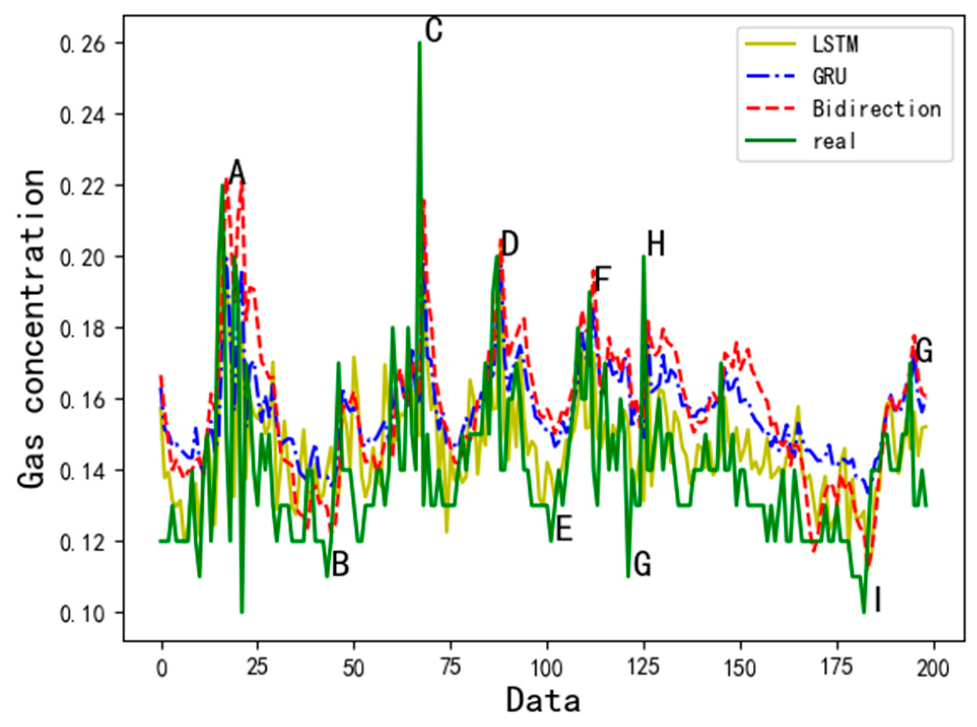
4.1. Model Comparison

In order to verify the advantages of the LSTM model in different types of cyclic neural networks, this paper replaces the hidden layer structure of the LSTM model with the BidirectionRNN [25] and GRU [26] structures and experiments with the same parameters. The results are shown in Figure 12 and Figure 13 and

Table 4. Comparison of operation results.

Model	Model Parameter	Operation Time	MSE
LSTM	Batch size = 50 2 nerve layers 128 neurons	5960 s	0.003298
GRU		4543 s	0.003475
Bidirection		19,000 s	0.00541

.

The loss values of LSTM and GRU are more stable and lower than those of BidirectionRNN in Figure 12. In

Table 5. Comparison of prediction results.

Model	Maximum Error	Minimum Error	Average Error
BidirectionRNN	0.067761	0.000572	0.022019
GRU	0.063648	0.000916	0.02246
LSTM	0.046283	0.000589	0.015979

, under the same model parameters, LSTM and GRU run time is shorter than Bidirection; in Figure 13, for GRU only some peak points and overall trends can be fitted, but the fitting effect at specific moments is not good. Bidirection can effectively fit the values of peaks A, C, D, F, and G, but in the valleys B and E, the fitting effect of G and I is far less than that of LSTM. Compared with GRU and Bidirection, LSTM can effectively fit not only the overall gas concentration change trend, but also the peak and trough values, and fit the time series. The error is minimal during the process of changing trends. LSTM is better than the GRU and Bidirection models for two reasons. First, both LSTM and GRU update and retain information through gate control. However, the parameters in GRU are less suitable for fewer samples, and there are more suitable samples in LSTM. Second, Bidirection has strong learning ability, but there is more complexity, requiring training samples to be larger and more time consuming.

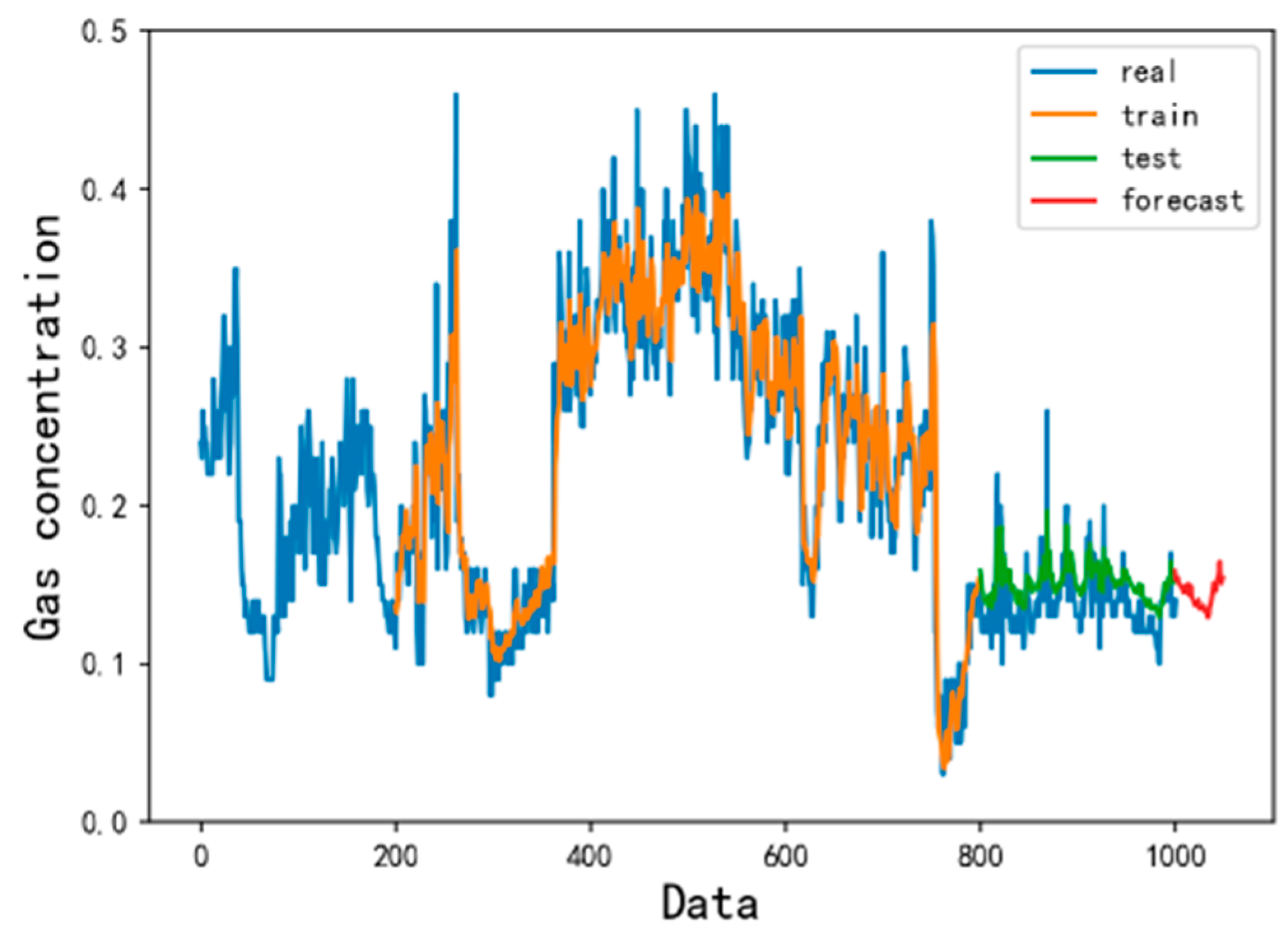
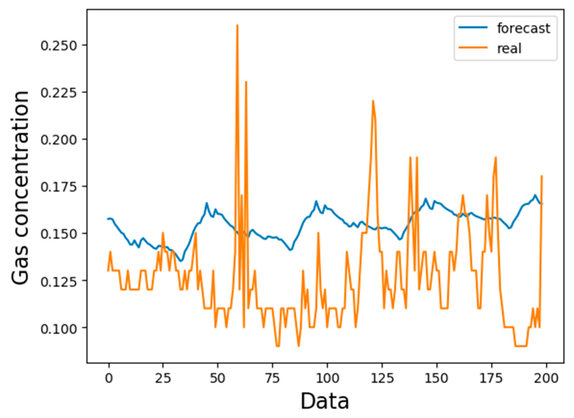
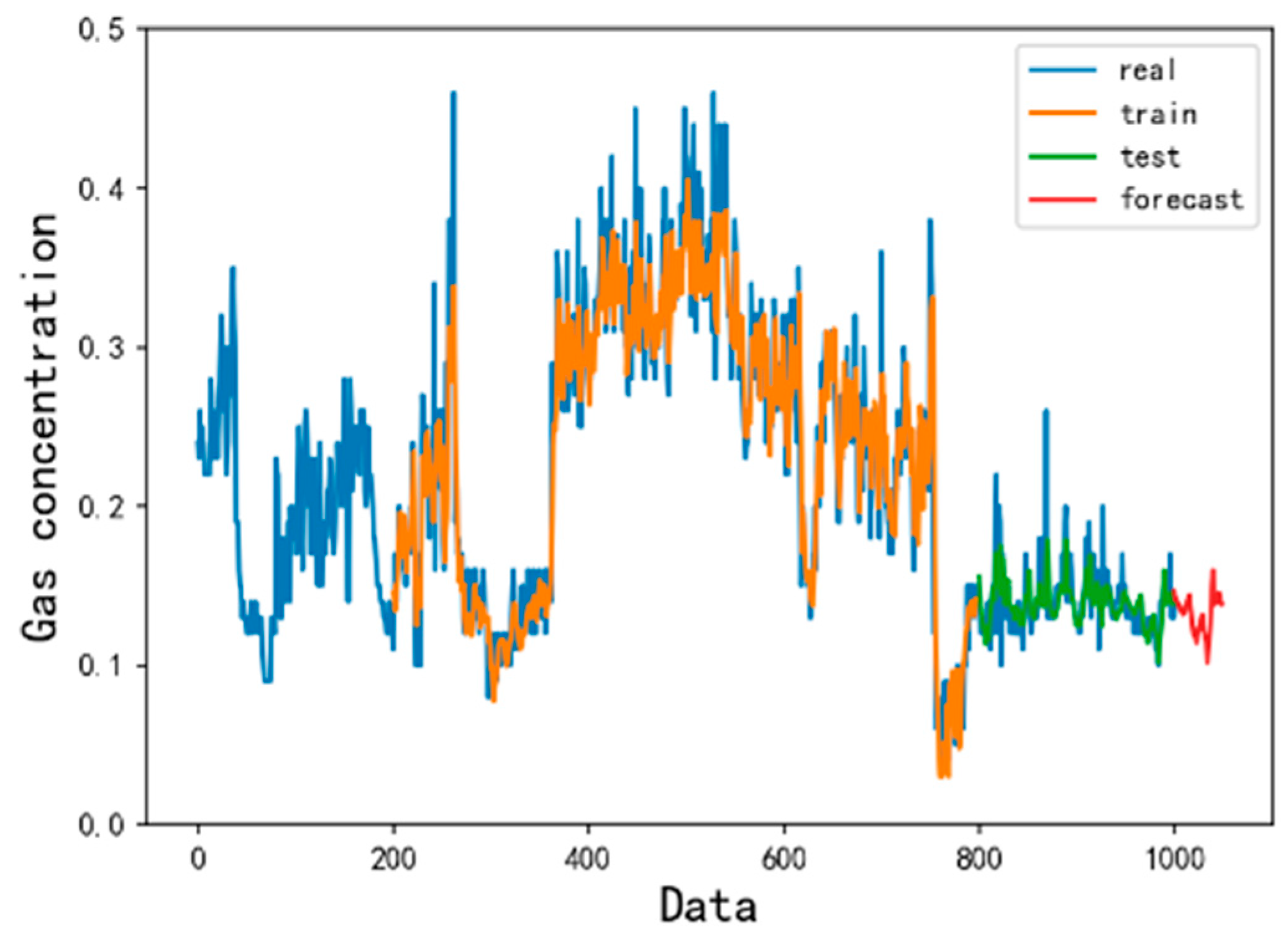
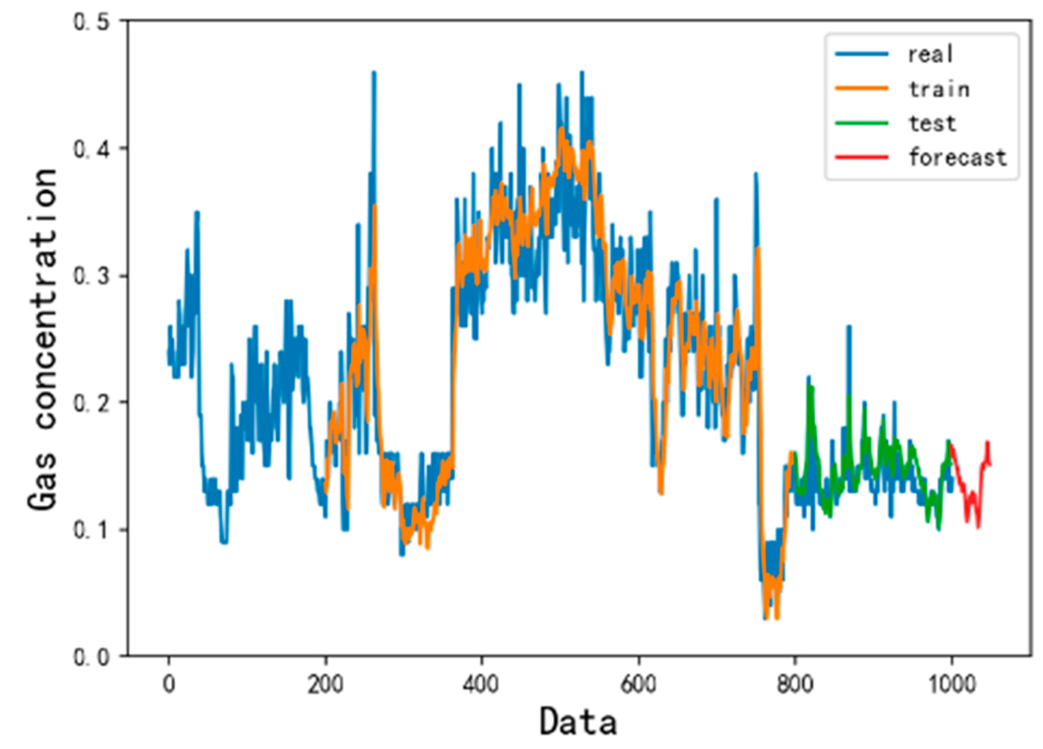
4.2. Forecast Results and Analysis

To further verify the superiority of the LSTM model, this paper compares the overall fitting effect and prediction results of LSTM with GRU and BidirectionRNN, as shown in Figure 14, Figure 15, Figure 16 and Figure 17. In the gas time series, GRU can better predict the trough value. The prediction result is lower than the true value in the peak of the time series; the Bidirection model predicts poorly and the overall prediction value is higher than the true value. LSTM is better: it predicts the overall trend of the gas time series, especially at the inflection point of gas concentration change, which can better reflect its superiority. Compared with the prediction results, LSTM is significantly better than BidirectionRNN and GRU. Although the three models can predict the overall change trend of gas concentration, the prediction error of the LSTM model is significantly smaller than that of the BidirectionRNN and GRU models. Table 5 shows a detailed comparison of prediction data errors. The BidirectionRNN and GRU prediction models are roughly similar. The maximum mean square error is 0.06, the minimum mean square error is 0.0005, and the mean square error is 0.02. The LSTM prediction model is more robust, with better saturation and higher accuracy, and the maximum and average mean square error can be reduced to 0.04 and 0.016, respectively.

In order to improve the practicability and reliability of the LSTM gas concentration prediction model proposed in this paper, the production monitoring data of other working faces in the Tingnan coal mine are selected for the LSTM gas concentration prediction model. The prediction results are shown in Figure 18.

Figure 18 shows the LSTM gas concentration prediction model. During the training process, the model learning ability was poor at the initial training time. As the parameter weights in the model were continuously optimized, the model learning ability was gradually enhanced, especially at the gas concentration time inflection point. The trend of gas concentration change can be well learned. During the test, the LSTM gas concentration prediction model better fit the variation trend of gas concentration time series, and the mean square error was reduced to 0.007. In the prediction process, the LSTM gas concentration prediction model predicted that the absolute error could be reduced to 0.006, and the predicted absolute mean square error fluctuation range was 0.004–0.026. In summary, the LSTM gas concentration prediction model can effectively predict the gas concentration change trend in the next time period in other application scenarios with high prediction accuracy and robustness and can be used for other applications.

5. Conclusions

From the results of this work the following conclusions may be proposed:

(1)

During the training process, the selection of batch size and number of LSTM layers has a great influence on the objective function value, fitting effect, and running time. The appropriate batch size and number of LSTM layers can effectively improve the model. Predicting the accuracy and fitting effect and reducing the training running time, the LSTM gas concentration prediction model in this experiment used a batch size of 50 and two LSTM layers as the optimal model parameters.

(2)

Compared with other cyclic neural network variants, BidirectionRNN and GRU prediction models, the effects of LSTM prediction are better, the average mean square error of the model can be reduced to 0.003, the predicted mean square error can be reduced to 0.015, and the predicted mean square error range is 0.0005–0.04, which has higher accuracy, robustness, and applicability.

(3)

The cyclic neural network can solve the time series problem, and the LSTM can solve the problem of gradient disappearance and gradient explosion and deal with the time series with long delay. For the gas concentration time series, the LSTM model can predict the concentration of gas in the next time period in a short time range, especially at the time inflection point of the gas concentration change, which can better reflect the LSTM prediction time series data, and the mean square error can be reduced to 0.005.

(4)

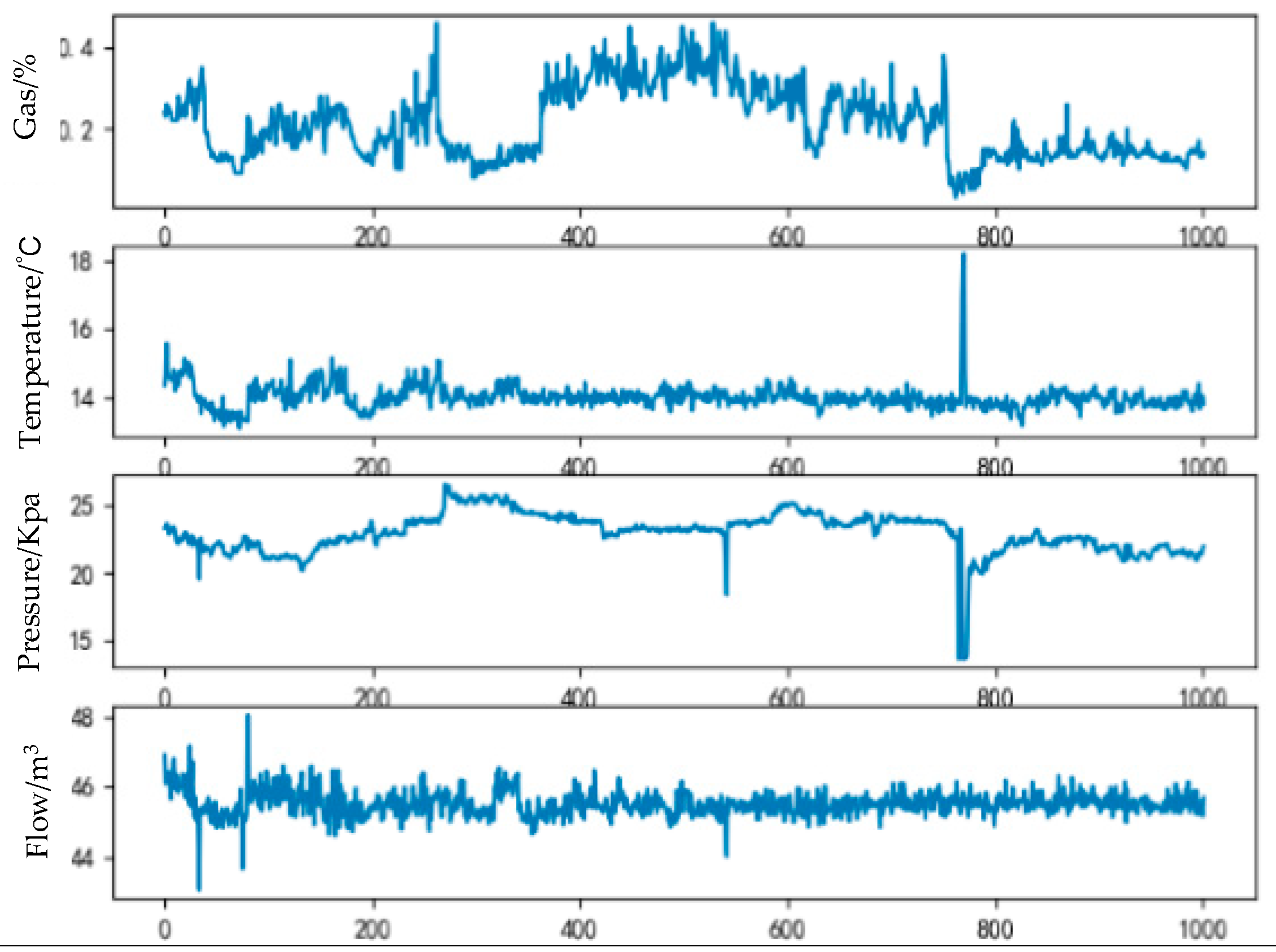
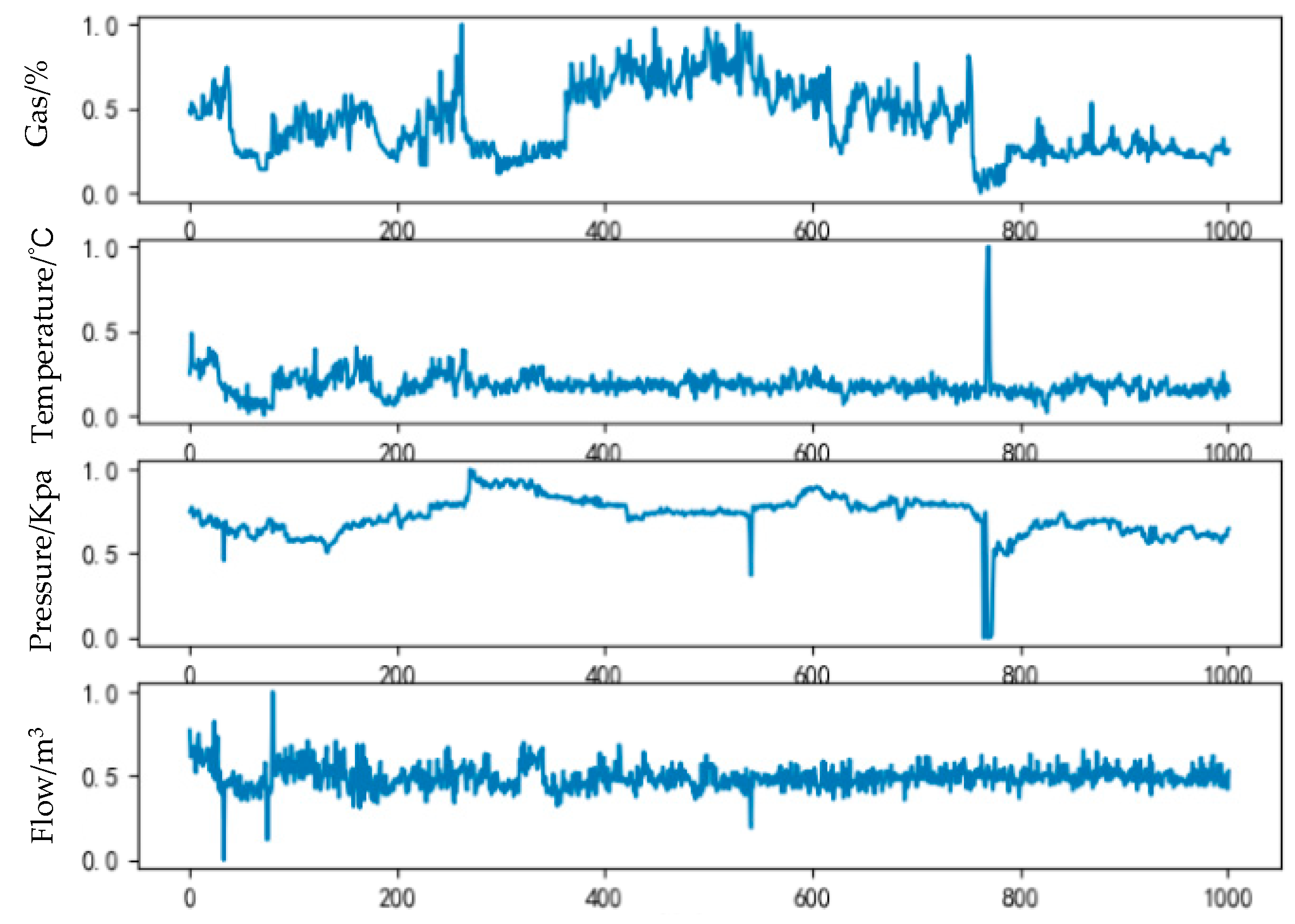
Compared with the traditional gas concentration prediction method, the model selects more monitoring data with longer samples and time spans as training samples. The LSTM prediction model has higher precision and wider application scenarios. At the same time, after learning the gas concentration time series law, the LSTM model can clearly predict the trend of gas concentration change in the next time period and provide a reference for coal mine safety.

References

1. Fu, H.; Dai, W. Dynamic Prediction Method of Gas Concentration in PSR-MK-LSSVM Based on ACPSO. J. Transduct. Technol. 2016, 29, 903–908. [Google Scholar]
2. Fu, H.; Feng, C.; Liu, J.; Tang, B. Study on Modeling and Simulation of Gas Concentration Prediction Based on DE-EDA-SVM. J. Transduct. Technol. 2016, 29, 285–289. [Google Scholar]
3. Wei, L.; Ling, L.; Fu, H.; Yin, Y. Dynamic Prediction Model of Gas Concentration Based on EMD-LSSVM. J. Saf. Environ. 2016, 16, 119–123. [Google Scholar]
4. Fu, H.; Zhai, H.; Meng, X.; Sun, W. A New Method for Gas Dynamic Prediction Based on EKF-WLS-SVR and Chaotic Time Series Analysis. J. Transduct. Technol. 2015, 28, 126–131. [Google Scholar]
5. Wu, Y.; Qiu, C.; Lü, X. Gas concentration prediction based on fuzzy information granulation and Markov correction. Coal Technol. 2018, 37, 173–175. [Google Scholar]
6. Liu, J.; Zhao, Q.; Hao, W. Study on Gas Concentration Prediction Based on Genetic Algorithm Optimized BP Neural Network. Min. Saf. Environ. Prot. 2015, 42, 56–60. [Google Scholar]
7. Guo, S.; Tao, Y.; Li, C. Dynamic Prediction of Gas Concentration Based on Time Series. Ind. Min. Autom. 2018, 44, 20–25. [Google Scholar]
8. Zhang, Z.; Qiao, J.; Yu, W. Real-time prediction method of gas concentration based on dynamic neural network. Control Eng. 2016, 23, 478–483. [Google Scholar]
9. Wang, X.; Wu, J.; Liu, C.; Yang, H.; Du, Y.; Niu, W. Fault Time Series Prediction Based on LSTM Recurrent Neural Network. J. Beijing Univ. Aeronaut. Astronaut. 2018, 44, 772–784. [Google Scholar]
10. Ma, X.; Tao, Z.; Wang, Y.; Yu, H.; Wang, Y. Long short-term memory neural network for traffic speed prediction using remote microwave sensor data. Transp. Res. 2015, 54, 187–197. [Google Scholar] [CrossRef]
11. Alex, G. Framewise phoneme classification with bidirectional LSTM and other neural network architectures. Neural Netw. 2005, 18, 602. [Google Scholar]
12. Dai, J.; Song, H.; Sheng, G.; Jiang, X.; Wang, J.; Chen, Y. Study on the operation state prediction method of power transformers using LSTM network. High Volt. Technol. 2018, 44, 1099–1106. [Google Scholar]
13. Li, P.; He, S.; Han, P.; Zheng, M.; Huang, M.; Sun, J. Short-term load forecasting of smart grid based on real-time electricity price based on long-term and short-term memory. Power Syst. Technol. 2018, 42, 4045–4052. [Google Scholar]
14. Song, K.; Hong, D. Short-term load forecasting for the holidays using fuzzy linear regression method. IEEE Trans. Power Syst. 2005, 20, 96–101. [Google Scholar] [CrossRef]
15. Pandey, A.; Singh, D.; Sinha, S. Intelligent hybrid wavelet models for short-term load forecasting. IEEE Trans. Power Syst. 2010, 25, 1266–1273. [Google Scholar] [CrossRef]
16. Wang, X.; Xu, L. Research on short-term traffic flow prediction based on deep learning. J. Transp. Syst. Eng. Eng. 2018, 18, 81–88. [Google Scholar]
17. Zhang, L.; Huang, S.; Shi, Z.; Rong, G. CAPCTA recognition method based on LSTM type RNN. Pattern Recognit. Artif. Intell. 2011, 24, 40–47. [Google Scholar]
18. Shi, W. Time Series Correlation and Information Entropy Analysis; Beijing Jiaotong University: Beijing, China, 2016. [Google Scholar]
19. Li, S.; Liu, L.; Yan, M. Improved particle swarm optimization algorithm for short-term traffic flow prediction based on BP neural network. Syst. Eng.—Theory Pract. 2012, 32, 2045–2049. [Google Scholar]
20. Yang, B.; Yin, K.; Du, J. Dynamic prediction model of landslide displacement based on time series and long and short time memory networks. Chin. J. Rock Mech. Eng. 2018, 10, 2334–2343. [Google Scholar]
21. Xu, C. Research on Multi-Granularity Analysis and Processing Method of Time Series Signal Based on Convolution-Long-Term Memory Neural Network; Harbin Institute of Technology: Harbin, China, 2017. [Google Scholar]
22. Xu, F.; Wang, Y.; Du, J.; Ye, J. Study on landslide displacement prediction model based on time series analysis. Chin. J. Rock Mech. Eng. 2011, 30, 746–751. [Google Scholar]
23. Zhao, X.; Song, Z. Adam optimized CNN super-resolution reconstruction. Comput. Sci. Explor. 2018, 12, 1–9. [Google Scholar]
24. Liu, W.; Liu, S.; Zhou, W. Research on Sub-Batch Learning Method of BP Neural Network. J. Intell. Syst. 2016, 11, 226–232. [Google Scholar]
25. Hao, Z.; Huang, H.; Cai, R.; Wen, W. Fine-grained Opinion Analysis Based on Multi-feature Fusion and Bidirectional RNN. Comput. Eng. 2018, 44, 199–204. [Google Scholar]
26. Li, X.; Duan, H.; Xu, M. Chinese word segmentation based on GRU neural network. J. Xiamen Univ. (Nat. Sci. Ed.) 2018, 12, 1–9. [Google Scholar]
Figure 1. Recurrent neural network (RNN) structure diagram.
Energies 12 00161 g001
Figure 2. Long short-term memory (LSTM) structural unit diagram.
Energies 12 00161 g002
Figure 3. LSTM gas prediction model framework.
Energies 12 00161 g003
Figure 4. Raw data.
Energies 12 00161 g004
Figure 5. Processed data.
Energies 12 00161 g005
Figure 6. Comparison of batch size loss. MSE, mean square error.
Energies 12 00161 g006
Figure 7. Comparison of batch size fitting effects.
Energies 12 00161 g007
Figure 8. Comparison of LSTM layer loss.
Energies 12 00161 g008
Figure 9. Comparison of LSTM layer number fitting effect.
Energies 12 00161 g009
Figure 10. Comparison of predicted length loss.
Energies 12 00161 g010
Figure 11. Prediction of length fitting results.
Energies 12 00161 g011
Figure 12. Comparison of loss for three models.
Energies 12 00161 g012
Figure 13. Comparison of test results for three models.
Energies 12 00161 g013
Figure 14. LSTM prediction model fitting effect diagram.
Energies 12 00161 g014
Figure 15. GRU prediction model fitting effect diagram.
Energies 12 00161 g015
Figure 16. BidirectionRNN prediction model fitting effect diagram.
Energies 12 00161 g016
Figure 17. Comparison of prediction results for three models.
Energies 12 00161 g017
Figure 18. Verifying the prediction results.
Energies 12 00161 g018