1. Introduction
Several studies have estimated Global Horizontal Irradiance (GHI) from various methods, but a higher temporal resolution of GHI is likely necessary for several applications such as photovoltaic panel and concentrated solar power projects. Recently, the demand for GHI has increased for solar energy projects. This is owing to problems related to non-renewable energies, a lack of other energy sources, increasing the use of energy and potential availability of solar energy [
1,
2,
3,
4]. Stations with long historical measurements of GHI are limited because of the cost of installation and maintenance, and issues related to the pyranometers [
5]. Therefore, several studies have tried to estimate GHI empirically from the early 20th century until now from other climate variables, namely, Sunshine Duration (SD), Air Temperature (AT), cloud cover, and other variables, using the top-of-atmosphere irradiance on the horizontal surface (TOA) [
6,
7,
8,
9,
10,
11] and with linear regression models [
12,
13,
14]. Recently, machine learning approaches have also been broadly used [
15,
16], which mostly include Artificial Neural Networks (ANNs), which will be discussed in a later section, Support Vector Machines, Random Forest [
5,
17,
18] and some other machine learning models [
19,
20]. Some of these and other approaches have used satellite image data and interpolation techniques to cover the limitation of spatial resolution [
3,
21,
22,
23].
Geostationary satellites such as Meteosat First Generation (MFG), Meteosat Second Generation (MSG)/Spinning Enhanced Visible, Infrared Imager (SEVIRI), the Japanese Geostationary Meteorological Satellite (GMS), and the Geostationary Operational Environmental Satellite system (GOES) are considered to be more acceptable for obtaining high temporal resolution of GHI data than other satellites. Heliosat-2 is a method that has been widely used for converting satellite images to GHI. The reader is referred to Refs [
24,
25] for further information about Heliosat-2. Some other approaches can also be found in the literature with the same aim [
26,
27]. Consequently, several datasets and services are providing GHI data with various spatial and temporal resolutions globally. More detailed information about them can be found in [
28]. The HelioClim-3 (HC3) and Copernicus Atmosphere Monitoring Service (CAMS) Radiation Service (CRS) are the most widely used Satellite-Derived Datasets (SDDs) which cover Europe, Africa and Asia [
29]. They provide GHI data at the sub-hourly scale and have been built using the Heliosat-2 and Heliosat-4 algorithms, respectively. Their data have been validated in several climate regions, with overall results that show good agreements with quality-controlled ground data [
30,
31,
32,
33]. Full information and its availability can be found in [
29]. Therefore, this study will use hourly GHI data from HC3 version-5 (HC3v5) and CRS version-3 (CRSv3) and combine them with climate variable ground data in an ANN algorithm for modelling GHI in areas where recorded GHI ground data are scarce.
SDDs have also been utilised with ground data to improve GHI datasets. For instance, Journee et al. in two different studies have merged SDD from MFG and MSG with GHI ground data to make a solar map over Belgium using kriging interpolation [
34,
35]. A map of GHI has been created by the combination of those datasets. SDDs are also important for other uses, such as for showing long-term trends of GHI over Europe and updating existing records [
36]. It has also been used for a crop estimation model [
37] and to obtain a coefficient of regression for calibrating a model for the same purpose [
38]. Those studies revealed that SDDs are affordable for improving the results of GHI estimation.
Other research has used ANN models to analyse satellite images for estimating GHI and other components of solar radiation. For example, Meteosat-6 images have been analysed to estimate monthly GHI over Turkey [
39]. Similarly, Meteosat-9 images have also been used with extra data in a model in Andalusia, Spain [
40]. ANNs have also been used with Heliosat-2 for converting multi-spectral MSG images to estimate hourly GHI [
41]. In addition, images from the Japanese Multifunctional Transport Satellites (MTSAT) have been analysed and combined with other data in an ANN for predicting GHI [
42]. Other studies have analysed satellite images for obtaining climate variable data (such as land surface temperature) which were then paired with ground measurements in a model to estimate GHI [
43,
44]. Another case is Qin et al. [
45], who input monthly precipitation calculated from TRMM satellite data with surface temperature from the Moderate Resolution Imaging Spectroradiometer (MODIS) to a model with GHI as an output. These papers have examined the use of ANNs with some climate parameters from satellite images to estimate GHI, but the high temporal availability of those parameters is limited.
ANNs have also been used to forecast GHI with various data and over various time intervals. For example, HC3, climate variables and other inputs have been analysed in ANN models to forecast GHI in intra-day and 1–6 h ahead in Gran Canary, Spain in two different studies [
46,
47]. They demonstrated that the SDD improved the forecasting results. Cloud properties and metric velocity data from satellite images with ground data have been used in an ANN model to forecast GHI at 30, 60, 90 and 120 min time scales [
48]. Clear sky irradiance on a horizontal surface (Cs) and weather research data have been used to forecast 24 h ahead with an ANN model [
49]. Hybrid ANN models have also been used to forecast one hour ahead [
2,
50]. Those papers demonstrated the role of ANNs in forecasting GHI at various time scales, and the role of SDDs and Cs as inputs to improve the model results. Another study has utilised machine learning algorisms to forecast GHI on a tilted panel based on several inputs namely climate variables, satellite data and solar position [
19].
ANNs are considered one of the most powerful algorithms to find relationships between dependent and independent variables. They have been used broadly in literature to estimate GHI and other solar components with different types of data. For instance, geographical and meteorological parameters at different time scales as various inputs have been used with ANN models for a variety of climate regions and countries. For example, two cities in Oman [
51]; eight cities [
52] and nine cities [
53] in China; 195 cities in Nigeria [
54]; 27 stations [
55], seven cities [
56] and 30 cities [
57] in Turkey; five stations in Argentina [
12]; six cities in the Yucatan peninsula, Mexico [
18]; five cities in Italy [
58]; four cities in the USA; and two cities [
59], 10 cities [
60] and 12 cities in Iran [
61]; and Cairo city in Egypt [
17]. Generally, the results of those models in the literature show good agreement with ground data. This indicates the importance of various types of ANN models and algorithms for estimating GHI. However, those studies mainly focused on daily timescales and in a few cases on monthly scales, not at an hourly time scale, which is the focus of this study.
After an extensive review of recent literature, only four studies have been found that have used ANNs to estimate GHI on the hourly timescale. The studies focused on one city each in Algeria [
62], Malaysia [
63] and Morocco [
64], and on five cities in North Africa and Jordan [
5]. They are fully described and compared to this study in
Table 1. On the other hand, other studies have estimated Direct Normal Irradiance (DNI) [
58,
65], Diffuse Horizontal Irradiance (DHI) [
66,
67] and have forecasted GHI, as mentioned in the previous paragraphs using ANN models on hourly time scales.
The studies (
Table 1) also used other machine learning approaches with ANNs, estimated other solar components and estimated timescales, whereas the descriptions in the table are focused on the ANNs for estimating hourly GHI.
It seems clear from the literature that studies using SDDs and combining them with observed climate variables (SD, AT, Relative Humidity (RH) and Wind Speed (WS)) and with TOA and Cs as several new input combinations in an ANN model to estimate hourly GHI are limited. The aim of this study was to model hourly GHI in areas with few ground measurements by using new input variable combinations, which have not been seen in the previously mentioned studies on hourly scales or even on daily scales.
3. Results
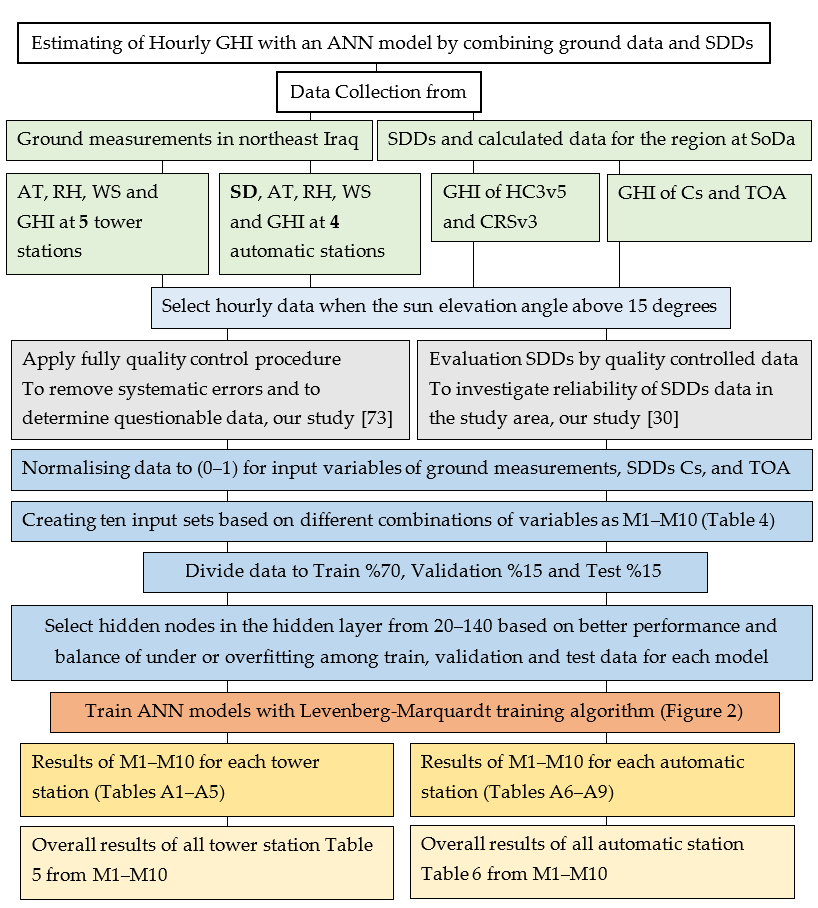
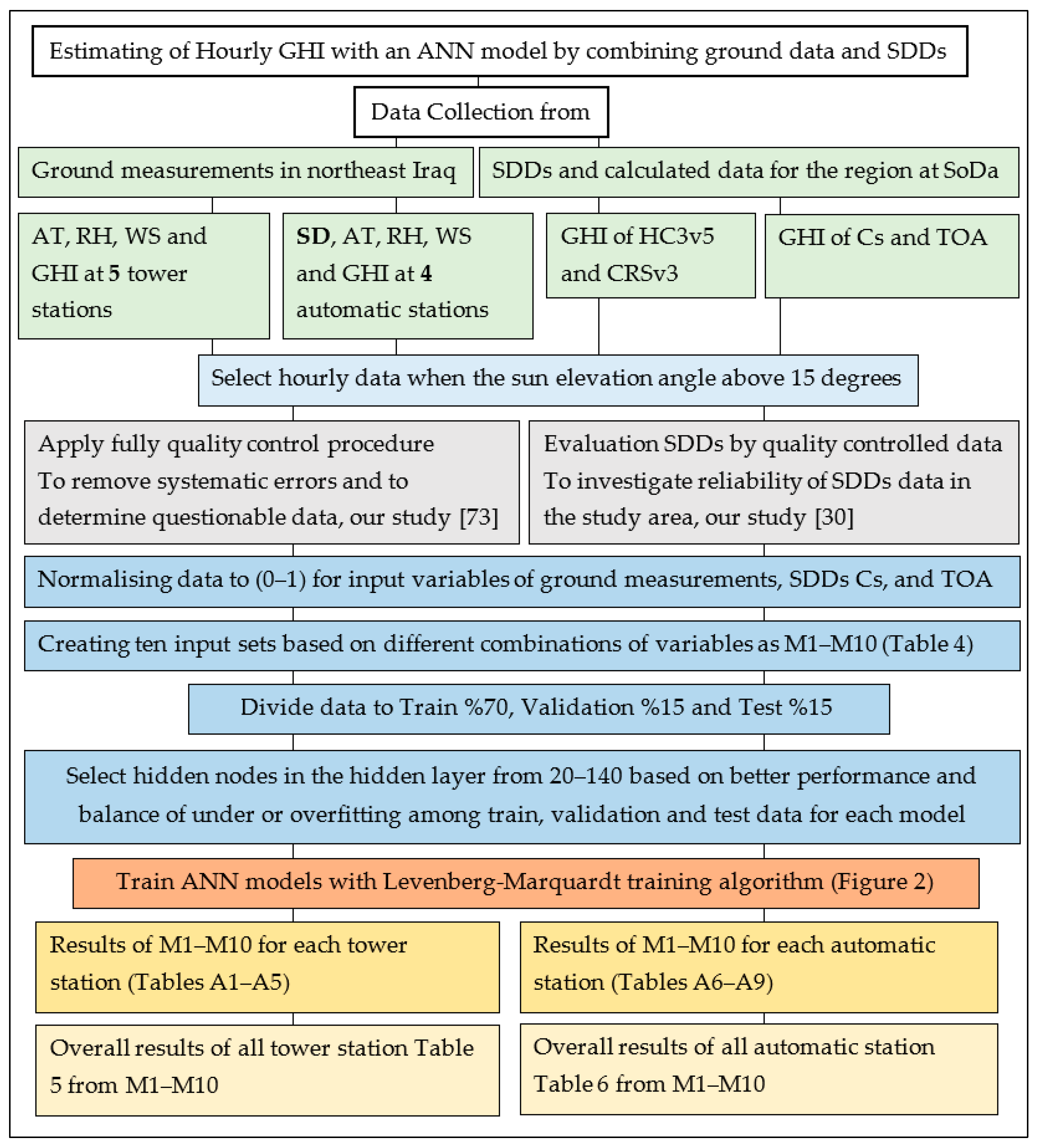
The results of hourly GHI with ANN models from M1–M10 based on variable inputs for training, validation and test data were averaged for four automatic stations and five tower stations and are presented in
Table 5 and
Table 6 respectively. However, the same results with the number of neurons in the hidden layer, number of datasets used and mean of GHI ground data for every individual station types are presented in
Table A1,
Table A2,
Table A3,
Table A4,
Table A5,
Table A6,
Table A7,
Table A8 and
Table A9 with two
Figure A1 and
Figure A2 of relative bias and RMSE of test data for further demonstration.
Figure 4 and
Figure 5 show a further comparison of the relative bias and RMSE between the models and the station types in the test data. In addition, the results of M1–M10 in the test data are shown with scatterplots of ground vs models and estimated vs residuals in
Figure 6,
Figure 7,
Figure 8 and
Figure 9 for both station types respectively.
As can be seen in
Table 5 (tower stations) and
Table 6 (automatic stations), there is no significant difference (the differences are lower than 3% in all individual cases) when comparing training and validation data with test data, which is in line with the stated methodology. Therefore, the results will be presented and discussed according to the models’ independent test data, which is more important to demonstrate the reliability of each model.
The lowest r value range among the models are 0.601 and 0.755 in M1 for both station types, respectively. The highest
r value is 0.983 in M9 automatic stations and 0.976 in M10 tower stations. Other
r values range from 0.903–0.982 in both station types (
Table 5 and
Table 6). Despite both high and low
r values, the values of M3 and M5 compared to other remaining values are low in automatic stations. This is also true for M2, M3 and M6 to others at tower stations.
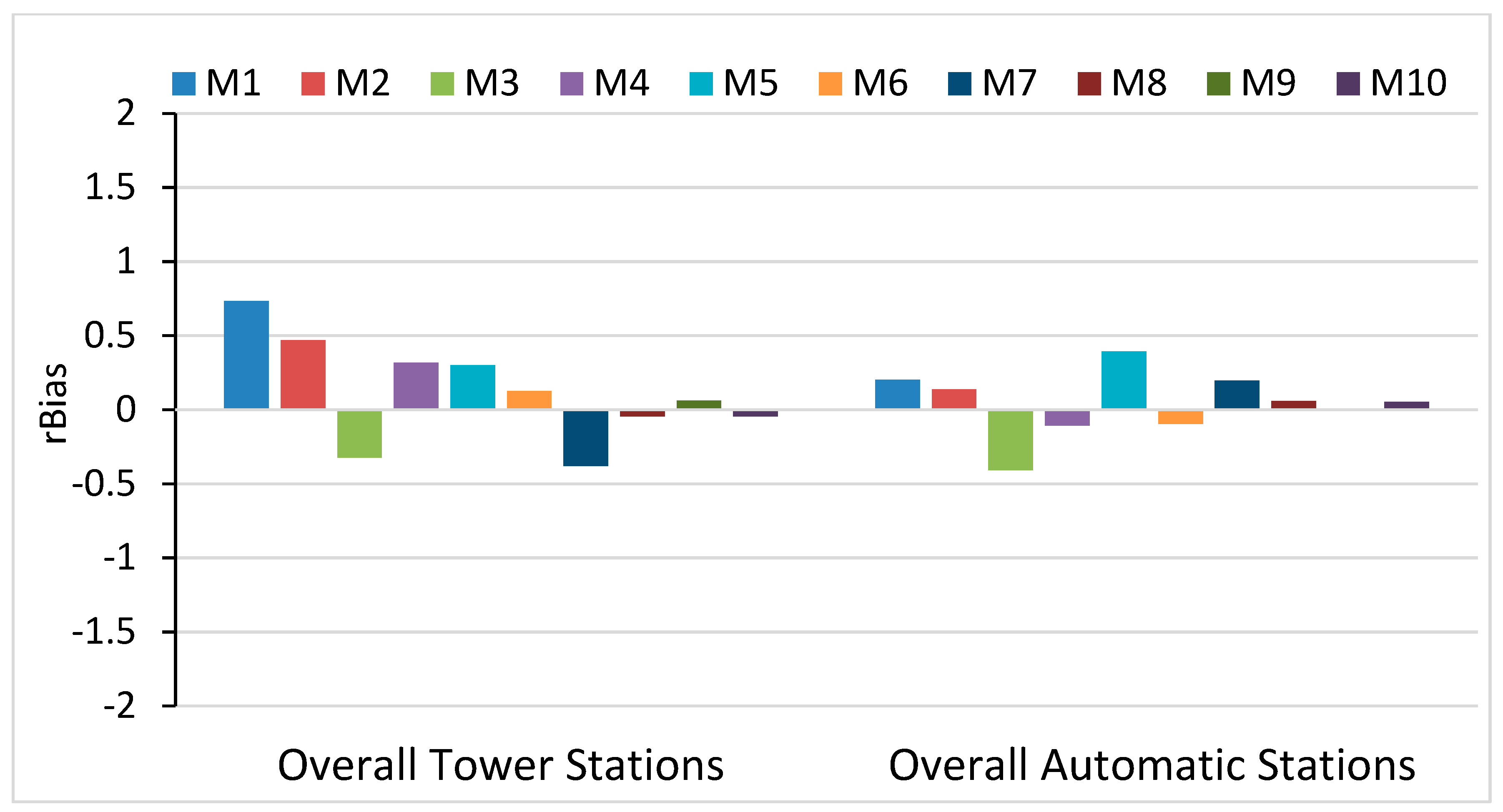
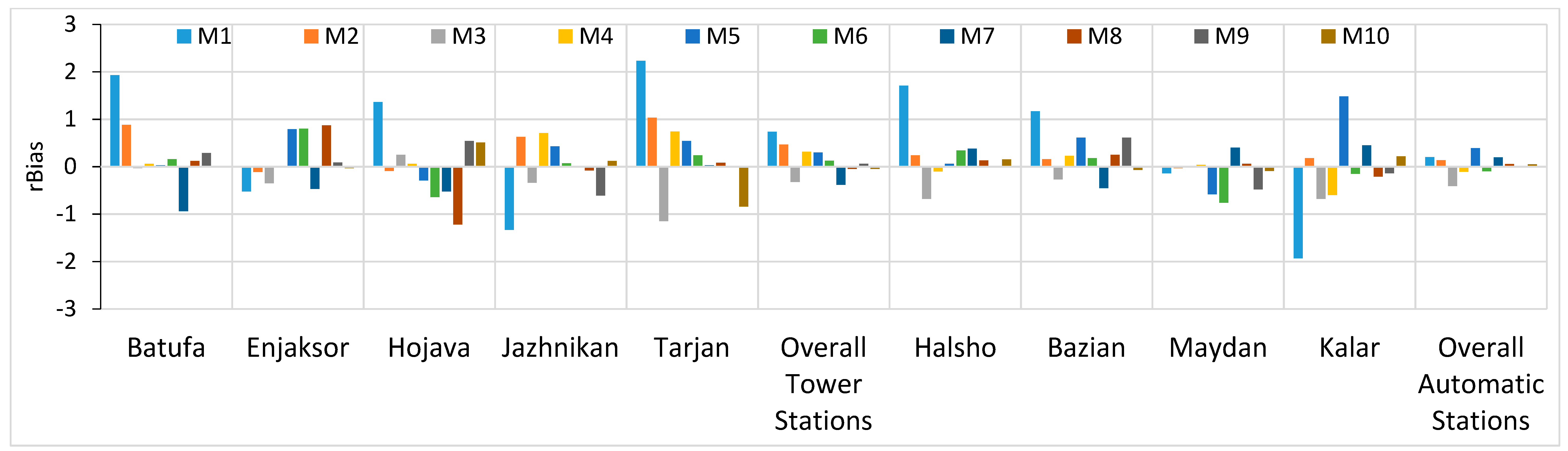
The values of bias were significantly low in all cases in the study area, which is under 1% of mean ground data for M1–M10. In the tower stations, the highest bias was recorded in M1 (3.4 W/m
2) 0.7%. It was 0.4% (2.3 W/m
2) in M2, a negative bias of −0.4% (−2 W/m
2) in M7 and the others’ rates were below 0.3%. However, in the automatic stations, the highest bias was recorded in M3 (−2 W/m
2) −0.4%. It was 0.3% in M1 and M5, and the others were below that value. The lowest bias was recorded at M8, M9 and M10, which were close to zero in both station types (
Table 5 and
Table 6,
Figure 4).
Figure 4 demonstrates the low rates of relative bias among M1-M10 for both station types.
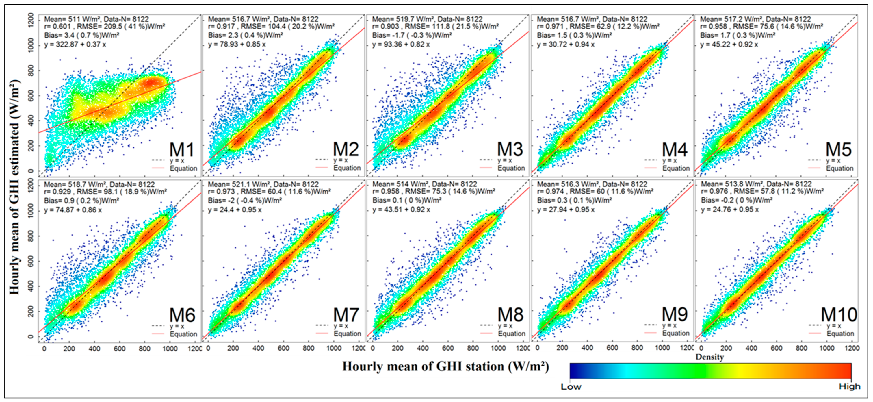
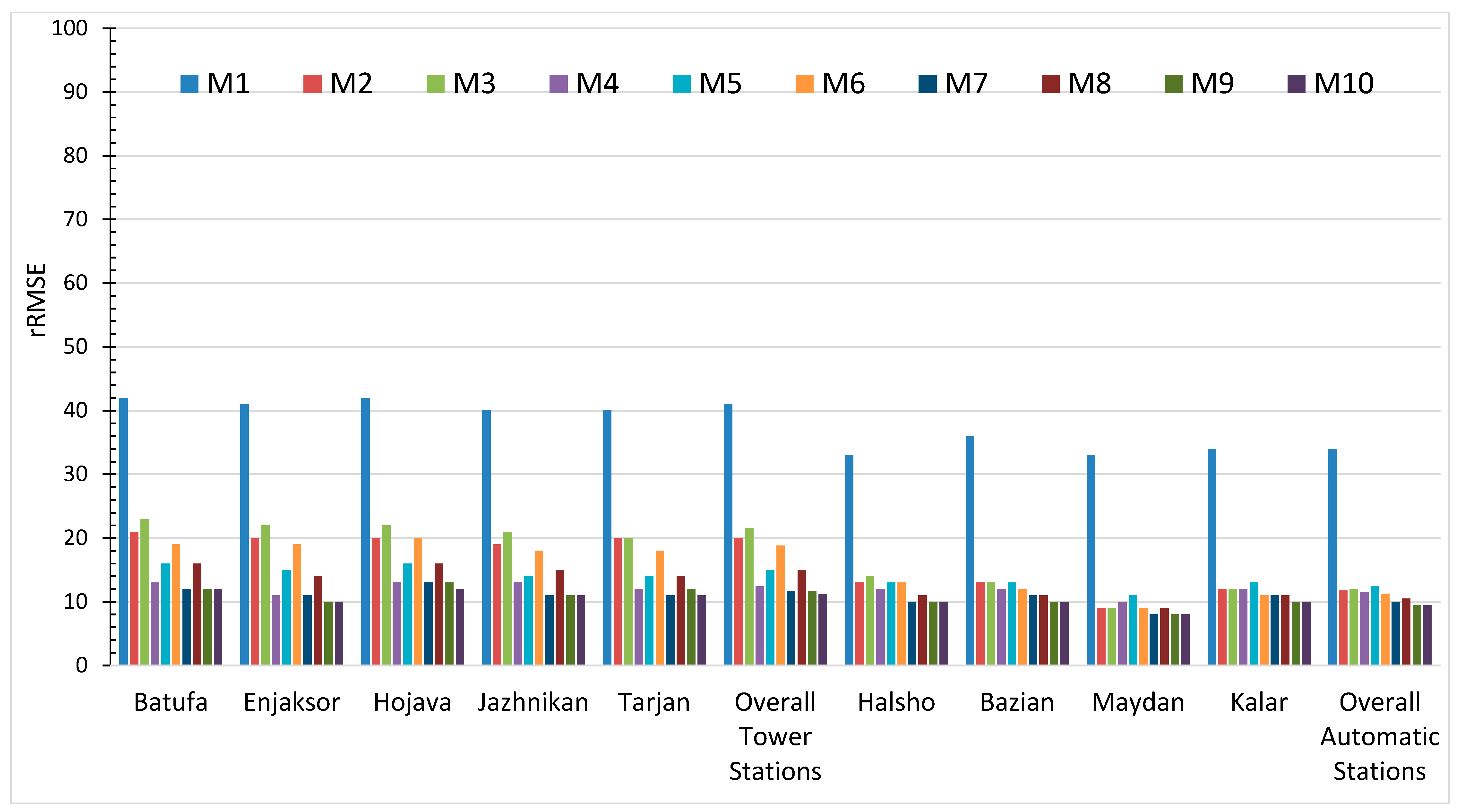
The RMSE results showed similarity with bias. The highest RMSE in tower stations was recorded in M1 (209.5 W/m2 41%). It decreased to 111.8 W/m2 (21.5%) and to 104.4 W/m2 (20.2%) in M3 and M2 respectively. The lowest recorded RMSE values were 57.8 W/m2 (11.2%), 60 W/m2 (11.6%) and 60.4 W/m2 (11.6%) in M10, M9 and M7 respectively. Other rates are between 12–19%.
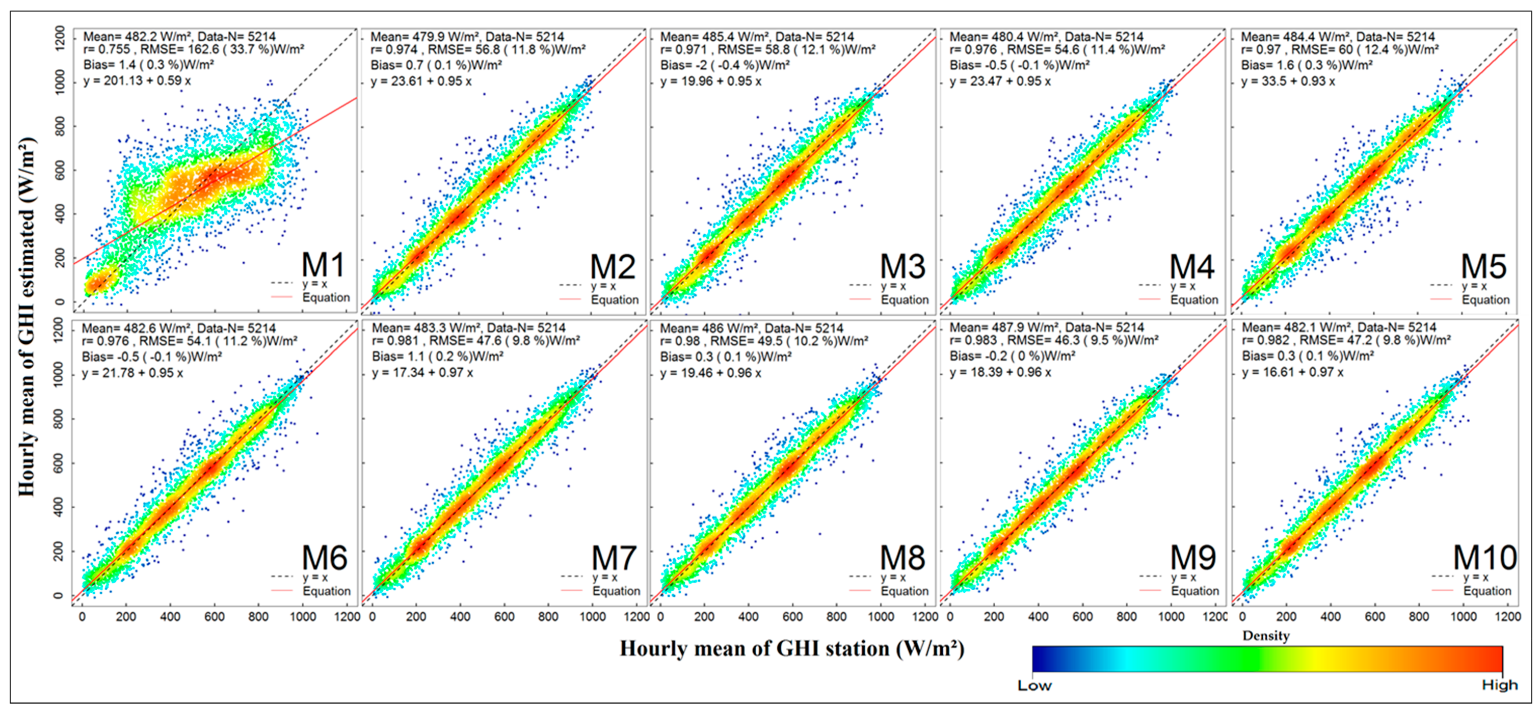
On the other hand, the RMSE at automatic stations are low compared to tower stations for each model. However, the highest one was recorded in M1 (163.6 W/m
2 33.7%). It decreased to 60 W/m
2 (12.4%) in M3. The lowest RMSE was recorded in M9 (46.3 W/m
2 9.5%) and there were slightly higher values in M7 (47.6 W/m
2 9.8%) and M10 (47.2 W/m
2 9.8%). The other remaining values were between 10–12% (
Table 5 and
Table 6,
Figure 5).
Figure 5 shows the stability of relative RMSE in automatic stations after M1 among the other models whereas it shows fluctuations for tower stations for the same situation.
Those rates of RMSE can be noted clearly by a close look at the scatterplots of each model in
Figure 6 (tower stations) and
Figure 8 (automatic stations), which are demonstrating the results of hourly GHI models in test data against ground measurements. The observations are concentrated around the 1:1 line in better performance models (M8, M9 and M10), where the regression lines are correspondingly close to the 1:1 line. The opposite is seen in M1 for both station types. However, in models M2, M3 and M6 (tower stations) the observations are far from the 1:1 line and the regression line in red is not close to the 1:1 line, corresponding to high recorded RMSE compared to other models (
Figure 6).
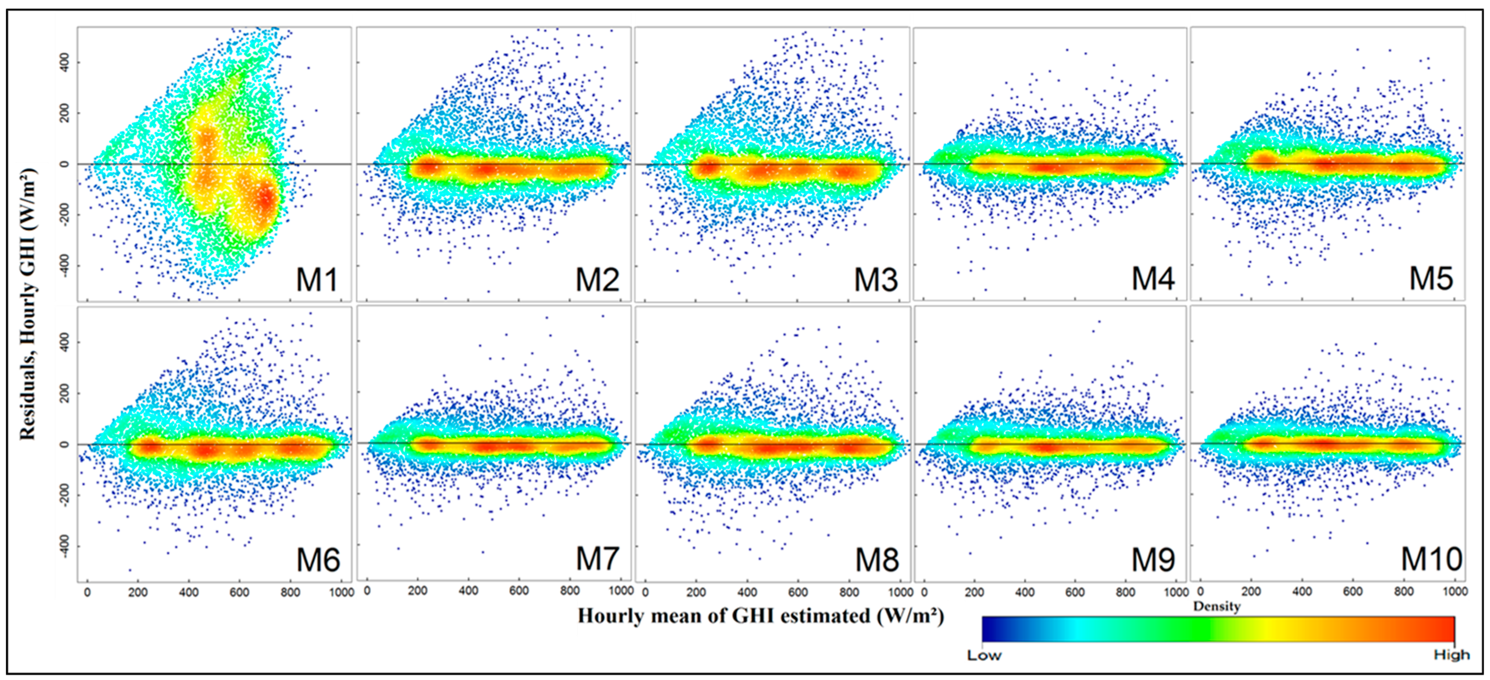
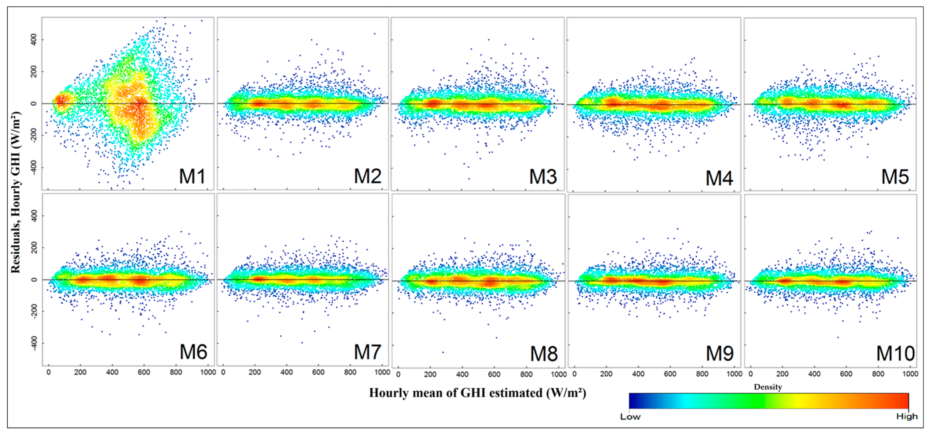
Figure 7 (for tower stations) and
Figure 9 (for automatic stations) show the scatterplots of residuals against estimated hourly GHI of test data in each model. The clustered patterns of residuals are seen only in M1 in both station types whereas all other residuals are randomly distributed and the densities of observation are around zero. However, low performance can be noted at M2, M3 and M6 (
Figure 7).
4. Discussion
The hourly GHI was estimated over nine stations in Iraq by using observed inputs (SD, AT, RH and WS), calculated inputs (TOA and Cs) and new input from SDDs (HC3v5 or CRSv3) to the ten M1-M10 ANN models based on the number and combination of inputs. The results of the overall performance are r values from 0.601–0.976, bias from −0.4–0.0–0.7% and RMSE from 11.2–41% at tower stations and r values from 0.755–0.983, bias from −0.4–0.0–0.3% and RMSE from 9.5–33.7% at automatic stations. Excellent performance was recorded in M9 (9.5%), and M10 (11.2%) and low performance was recorded in M1 at automatic and tower stations respectively. The better results of those models at hourly time scales compared to the previous studies for similar estimation (
Table 1) are related to the new inputs such as Cs, TOA and SDDs together in this study.
The overall better performance, with a lower percent of automatic stations than tower stations in all models, is obtained by the use of SD as inputs in automatic stations—SD is unrecorded in tower stations. It is also reported [
6,
62,
64,
77] that the role of SD increases the performance of models.
The low performance of M1 in both station types is related to the small number of inputs, which do not include any of the calculated inputs. The calculated inputs such as Cs have a unique role to increase the model performance as seen in M2 compared to M1 in both stations. This is in agreement to improved results in some limited studies which used Cs as inputs either for modelling or forecasting GHI [
47,
49,
78,
79].
The low recorded bias in most of the models is related to the good estimation of GHI by ANN models as mentioned in several studies [
12,
17,
62,
64]. We presented the overall bias among stations, which led to a decrease in the bias because of positive bias in some stations and negative bias in others in the same model, whereas the bias in all individual stations was lower than 2% except one case of 2.2% (
Table A1,
Table A2,
Table A3,
Table A4,
Table A5,
Table A6,
Table A7,
Table A8 and
Table A9,
Figure A1).
The fluctuation of RMSE among models at tower stations and its stability among models at automatic stations (
Figure 5 and
Figure A2,
Table 5 and
Table 6) are mainly related to the role of SD, which was used as input in the later ones. The highest record of RMSE in M1 in both station types is related to inputs which contain only four climate variables. This is reported by literature where GHI was estimated at a daily time scale [
55,
77]. The improved performance in M2 and M3 compared to M1 is related to the use of additional variables of Cs and TOA in those models respectively (
Table 4). Hence, the low performance of M2, M3 and M6 compared to better performance in M4 and M5 are related to the use of SDDs as new inputs with climate variables. This has been reported by studies which have used SDDs in foresting GHI [
46,
47]. The better performance of M7 and M8 compared to the previous M1–M6 is related to the use of Cs with SDDs in those models. The role of Cs is mentioned in literature [
49,
79], but in those cases, it was not combined with SDDs. The overall better performances of M9 and M10 from the other models (M1–M8) are related to the combination of all variables in those models. These demonstrate the better performance of this study compared to similar studies [
5,
62,
63,
64].
The performance of HC3v5 as input with only four climate variables is better than CRSv3 as demonstrated in the comparison between M4 and M5 in both station types, whereas in other models (M7–M10) the difference between them are minimal. The former result (M4–M5) is related to the accurate reproduction of the GHI ground data by HC3v5 as described in the literature [
30,
32,
33]. The latter (M7–M10) is related to the use of Cs and TOA as separate inputs.
This study revealed that using SDDs, Cs, and TOA with climate variables in ANN models has improved the results of estimation for hourly GHI with an overall r value of 0.980, bias lower than 2% and RMSE lower than 10% compared to similar studies with no combination of those inputs [
5,
62,
63,
64].
The results of this study demonstrate that this way of modelling allows the retrieval or management of a dataset of GHI for decades where the inputs are available, but where GHI is not recorded as in most areas in the case study and similar regions with a scarcity of ground data, it can be achieved by using the trained models.
The new inputs of SDDs and Cs which improved the results are easily and openly available for most regions [
29] unlike other variables such as cloud cover and SD [
21,
73,
80]. Therefore, the mentioned new variables can be used for modelling and forecasting the solar components for better results.
The limitations are principally as follows: This study estimated GHI but no other solar components, which are required directly in fields such as DNI in concentrated solar power. Hence, some studies have estimated DNI and DHI from GHI [
64,
81,
82]. However, further research is required for that in this type of area with a scarcity of ground data. Another limitation is the scarcity of long-term GHI ground data at timescales beyond five years or more, which are better for training this kind of model.
5. Conclusions
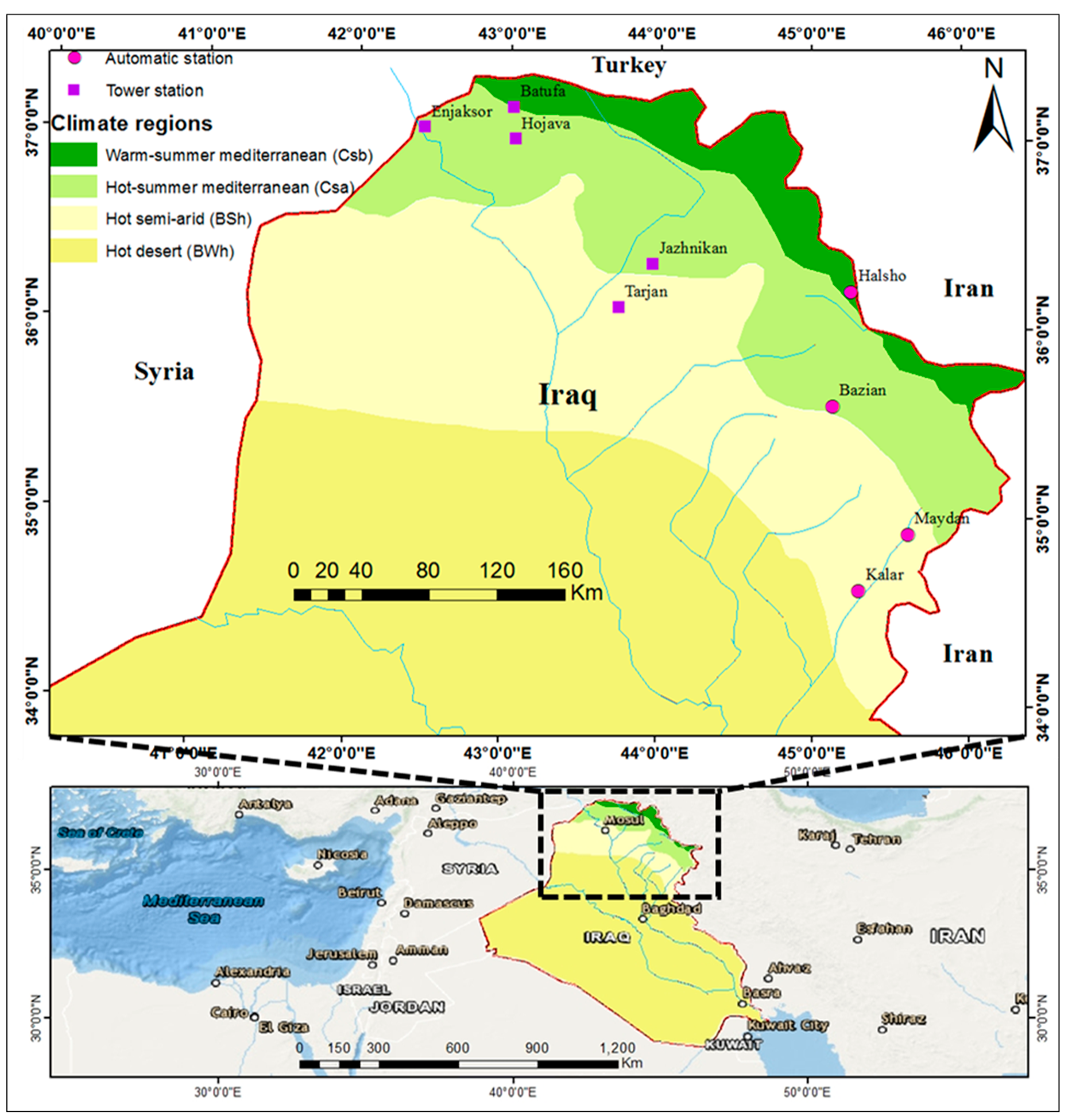
This paper aimed to use a new input of SDDs together with Cs, TOA and observed climate variables SD, AT, RH and WS as new input combinations in ten ANN models to estimate GHI at the hourly time scale with a Levenberg–Marquardt training algorithm. The inputs were arranged into ten different sets, as models M1–M10, to demonstrate the role of new inputs. The data at four automatic stations of all the above variables and five tower stations without SD in northeast Iraq were used.
The test results demonstrated a good improvement from M1 to M10 based on adding the new inputs such as TOA with observed variables (M3), Cs with observed variables (M2), SDDs with all observed climate variables (M4–M5), other combinations (M6–M8) and all together (M9–M10) with low percent fluctuation between both station types. The best results are r = 0.983, RMSE = 9.5% and bias = 0.0% in M9 and r = 0.976, RMSE = 11.2% and bias = 0.0% in M10 and the worst results are r = 0.755, RMSE = 33.7% and bias = 0.3% in M1 and r = 0.601, RMSE = 41% and bias = 0.7% in M1 at automatic and tower stations, respectively.
This study demonstrated the role of new input combinations for estimating hourly GHI with high accuracy. While the models have been trained with a few years of data, it would be better to train them with more years of data with such algorithms.
Further research is required for using new inputs with other machine learning approaches and empirical models.


