Data-Driven Kernel Extreme Learning Machine Method for the Location and Capacity Planning of Distributed Generation

Abstract

For the integration of distributed generations such as large-scale wind and photovoltaic power generation, the characteristics of the distribution network are fundamentally changed. The intermittence, variability, and uncertainty of wind and photovoltaic power generation make the adjustment of the network peak load and the smooth control of power become the key issues of the distribution network to accept various types of distributed power. This paper uses data-driven thinking to describe the uncertainty of scenery output, and introduces it into the power flow calculation of distribution network with multi-class DG, improving the processing ability of data, so as to better predict DG output. For the problem of network stability and operational control complexity caused by DG access, using KELM algorithm to simplify the complexity of the model and improve the speed and accuracy. By training and testing the KELM model, various DG configuration schemes that satisfy the minimum network loss and constraints are given, and the voltage stability evaluation index is introduced to evaluate the results. The general recommendation for DG configuration is obtained. That is, DG is more suitable for accessing the lower point of the network voltage or the end of the network. By configuring the appropriate capacity, it can reduce the network loss, improve the network voltage stability, and the quality of the power supply. Finally, the IEEE33&69-bus radial distribution system is used to simulate, and the results are compared with the existing particle swarm optimization (PSO), genetic algorithm (GA), and support vector machine (SVM). The feasibility and effectiveness of the proposed model and method are verified.

1. Introduction

The world’s energy sources are accelerating in their transition to diversification, cleanliness, and low carbonization. A hot topic in power systems is the high proportion of renewable energy power generation. In recent years, a large proportion of renewable energy has been connected to the grid, but its power generation output is random, which means the analysis and control of power system has become more important. This fundamentally changes the planning and operation characteristics of a distribution network. Therefore, studying the problem of distributed generation (DG) location selection and capacity is of value for the stability and economic operation of distribution networks.

The issues of DG location and capacity selection have received worldwide attention. Mahmoud et al. [1] and Ehsan and Yang [2] reviewed the benefits of distributed generation in terms of power supply efficiency, power quality improvement, stability, and safety, and pointed out that these benefits are mainly determined by the optimal configuration of the location and capacity of distributed power sources. The influence of wind power generation on voltage distribution and the active loss of the distribution network was studied by Vita et al. [3]. Vita [4] proposed a decision algorithm for distributed power sources’ location and capacity selection, which can be flexibly modified to adapt to different types of DGs. Asimakopoulou, G.E. et al. [5], from the perspective of the power market, an aggregation technology was proposed to quantify the benefits of large-scale DG access to the distribution network. Baghayipour, M.R. et al. [6], in order to solve the layout problem of wind power generation in the distribution network, presented a model considering the dynamic demand of nodes, the amplitude of node voltage, and the variation of wind speed was proposed. Li, M. et al. [7] and Wang, L [8] studied problems of grid-connected distributed power from the perspective of distributed power output and power distribution system adjustment capability. Chao, Q. et al. [9] proposed an optimization planning model for multi-energy systems based on the coupling of wind, solar, cold, heat, and power systems. Multi-stage planning and multi-scenario analyses were carried out with the goal of economic operation and investment cost optimization. Li, P. et al. [10] proposed an improved neural network model that effectively describes the external characteristics of various distributed power sources and meets the needs of engineering simulation. Fu, Y. et al. [11], an improved clustering algorithm was proposed for problems associated with clustering methods in the location and capacity of offshore wind farms. A second-layer optimization method for access systems, including substation site selection and grid topology planning, was proposed. Zhu, J. et al. [12], with the goal of the highest economic return on investment cycle, a distributed power supply location and capacity optimization method considering network dynamic reconfiguration was proposed.

It can be seen from the above references that the kinds of DG location and capacity selection models have been constructed, and the optimization algorithm such as particle swarm optimization (PSO) and genetic algorithm (GA) are applied to solve the model. However, with the development of research, some characteristics inherent in optimization algorithms have gradually become bottlenecks, restricting its further development. For example, the training speed is slow and time-consuming; it is easy to fall into local minimum, easy to produce premature convergence, local optimization ability is not strong; and parameter setting is complex, difficult, and has certain dependence on the initial population selection. In response to the above problems, Huang, G.B. et al. [13] proposed a new type of single hidden layer feed forward neural network (SLFN)-extreme learning machine (ELM). The algorithm has the advantages of fast learning speed, simple and easy to implement structure, less human intervention, and strong generalization ability. Ren, R. et al. [14], an optimized kernel extreme learning machine (KELM) method was proposed for the power load forecasting problem. Compared with support vector machine (SVM), the proposed method had good predictive performance and computation speed.

The rapid development of data analysis and processing technology have enabled a large amount of operational power system data to be accumulated, which laid a good foundation for data-driven analysis. The application of data-driven ideas and technologies to traditional power network analysis and optimization problems comprehensively uses historical and measured data, improving the accuracy of the results of power network analysis and optimization, thus improving the economical and stability of the power system. For issues of data quality and computational efficiency of intelligent transportation systems based on big data, Shen, K. et al. [15] summarized the development trends and the direction of advanced technologies, such as multi-source data fusion and multi-scenario applications. At present, few studies involve data-driven power flow calculations. For transmission networks, it is easier to establish a power flow calculation equation based on physical models. However, for distribution networks, due to the complex topology, the obtained information is usually incomplete, so it is difficult to perform power flow calculations based on accurate physical models. The access of a large number of distributed generation points makes the distribution network more uncertain. Therefore, considering the use of data-driven ideas, using historical and measured data to compensate for the completeness of information, through the training and testing of the model can help to solve the uncertainty description problem.

Therefore, we considered the use of data-driven thinking to describe the uncertainty of wind and photovoltaic output and introduced it into the power flow calculation of distribution networks. The multi-type DG location and capacity selection model based on the kernel extreme learning machine (KELM) was constructed to map various DG outputs to node voltages. Using the data-driven KELM method, various DG configuration schemes satisfying the constraints are provided and the voltage stability evaluation index is introduced to evaluate the results. The IEEE33&69-bus radial distribution system is used as an example to simulate and compare the obtained DG location and capacity selection results with particle swarm optimization (PSO) and genetic algorithm (GA) algorithms. The validity and feasibility of the proposed method were verified, and the computation speed was faster.

2. Location and Capacity Selection Model of DG

First, we discuss the stochastic models for wind and photovoltaic power generation.

2.1. DG Probability Model

2.1.1. Wind Power Generation

The output power of wind is affected by wind speed. Wind speed distribution obeys the Weibull distribution, and its probability density function [16] can be expressed by Equation (1)

$$f\left(v\right)=\frac{k}{c}{\left(\frac{v}{c}\right)}^{k-1}exp\left[-{\left(\frac{v}{c}\right)}^k\right]$$

(1)

where k and c are the shape parameter and scale parameter of the Weibull distribution, respectively, and v is the actual wind speed.

The wind power, as a function of the wind speed, is a non-linear function, so this linear power (speed) function is an approximation. Thereby, the output power distribution function P_w of the wind power generation can be obtained as

$$P_w=\{\begin{array}{cc}0& v\le v_{ci},v\ge v_{co}\\ P_n\left(v-v_{ci}\right)/\left(v_n-v_{ci}\right)& v_{ci}\le v\le v_n\\ P_n& v_n\le v\le v_{co}\end{array}$$

(2)

where v_ci is the cut-in wind speed, v_co is the cut-out wind speed, and P_n is the rated output of the fan. v_n is the rated wind speed.

2.1.2. Photovoltaic (PV) Power Generation

The solar light intensity s approximates the Weibull distribution over a certain period of time, and its probability density function [17] can be expressed as

$$f\left(s\right)=\frac{k}{c}{\left(\frac{s}{c}\right)}^{k-1}exp\left[-{\left(\frac{s}{c}\right)}^k\right]$$

(3)

where k and c are shape parameter and scale parameter, respectively.

Thereby, the output power distribution function P_s of the photovoltaic power generation can be obtained as

$$P_s=\{\begin{array}{cc}{P}_{sn}\left(s/s_n\right)& 0\le s\le s_n\\ P_{sn}& s\ge s_n\end{array}$$

(4)

s_n is the light intensity at the rated output power, and P_sn is the rated output power of the photovoltaic cell.

2.2. Voltage Stability Evaluation Index

The feasible critical solution to the current flow equation is considered the limit point of voltage stability. The voltage stability index is judged by the extreme conditions of the power flow solution, which can reflect the area where the system is the most prone to voltage collapse and the node [18]. Prior research [19] showed that the voltage stability of the whole system can be evaluated according to the index. The larger the index value, the more unstable the network voltage. We used an improved voltage stability index (IVSE). The index is calculated as

$$\mathrm{IVSE}=\frac{4Q\left(r^2+x^2\right)}{x{U}^2}$$

(5)

where Q represents the reactive power loss in the system; r and x represent the equivalent resistance and reactance of the system considering DG, respectively; and U represents the node voltage.

When the DG is not connected, the pre-pushback generation method is used to calculate the power flow of the distribution network. The voltage stability evaluation index is used as the reference value. The node with the largest index value was selected as the initial position of the DG access.

In order to facilitate comparative analysis, the rate of change of IVSE index is defined as

$$I_{ivse\_Rate}=\frac{\left|I_{ivse}-I_{ivse0}\right|}{I_{ivse0}}\times 100\%$$

(6)

where I_ivse0 indicates the initial value of the IVSE indicator when the DG is not connected, I_ivse indicates the value of the IVSE indicator under different DG configuration schemes, and I_{ivse_Rate} represents the rate of change of the IVSE indicator. The rate of change of the index indicates the change in the voltage of different nodes with access to the DG; the larger the value, the greater the degree of change at the access node.

2.3. Active Power Loss

For a radiating distribution network with n branches, the active power loss P_loss is

$$S_{ij}^2=P_{ij}^2+Q_{ij}^2$$

(7)

$$P_{loss}={\displaystyle \sum }_{i=1}^n\frac{S_{ij}^2}{U_i^2}{R}_{ij}={\displaystyle \sum }_{i=1}^n\frac{P_{ij}^2+Q_{ij}^2}{U_i^2}{R}_{ij}$$

(8)

where P_ij and Q_ij are the active and reactive power flowing through the branch, respectively; R_ij is the branch resistance; S_ij is the power flowing through the branch between node i and node j; and U_i is the voltage of node i.

After the DG is connected to the system, the input power to the node i is P_k, then

$$P_k=P_{wind}+P_{pv}$$

(9)

where P_wind and P_pv represent the output power of wind and photovoltaic power generations, respectively.

$$P_{loss}^{\prime }={\displaystyle \sum }_{i=1}^k\frac{{\left(P_i-P_k\right)}^2}{U_i^2}{R}_i+{\displaystyle \sum }_{i=k+1}^n\frac{P_i^2}{U_i^2}{R}_i+{\displaystyle \sum }_{i=1}^n\frac{Q_i^2}{U_i^2}{R}_i$$

(10)

Substituting Equation (9) and simplifying it to

$$P_{loss}^{\prime }=P_{loss}+{\displaystyle \sum }_{i=1}^k\frac{P_k^2}{U_i^2}{R}_i-{\displaystyle \sum }_{i=1}^k\frac{2P_i{P}_k}{U_i^2}{R}_i$$

(11)

where P’_loss represents the active power loss after DG access.

When the DG is not connected, the power flow calculation of the distribution network is performed, and the obtained value is used as the active power loss reference value of the distribution network system.

2.4. Restriction Conditions

Comprehensively comparing the composition of various objective functions, the active power loss is usually the basis of various objective functions. Therefore, in order to compare the simulation results, we used the chance constrained programming method to construct the objective function with the minimum loss of active power.

2.4.1. Opportunity Constraints

Considering the location and capacity study of DG uncertain factors, the node voltage amplitude and the feeder transmission capacity are generally allowed to have a few exceptions within a reasonable confidence level [20], as

$$P_r\left\{U_{min}\le U_i\le U_{max}\right\}\ge \alpha$$

(12)

$$P_r\left\{S_{ij}\le S_{ijmax}\right\}\ge \beta$$

(13)

where α and β take 0.95 according to practical experience in similar cases; U_max and U_min are the upper and lower voltage limits, respectively; and S_ijmax is the maximum line power transmission limit.

2.4.2. Equality Constraints

The equality constraint is based on the basic power flow equation of the distribution network, and influences the DG

$$\{\begin{array}{c}{P}_i+P_{DG}-P_{Li}-U_i{\displaystyle {\displaystyle \sum }_{jϵi}}{U}_j\left(G_{ij}\cos {\theta }_{ij}+B_{ij}\sin {\theta }_{ij}\right)=0\\ Q_i+Q_{DG}-Q_{Li}-U_i{\displaystyle \sum }_{}{U}_j\left(G_{ij}\sin {\theta }_{ij}-B_{ij}\cos {\theta }_{ij}\right)=0\end{array}$$

(14)

where P_i and Q_i are the active power and reactive power injected by the network to node i, respectively; P_DG and Q_DG are the active power and reactive power injected by DG to node i, respectively; P_Li and Q_Li are the active load power and reactive load power of node I, respectively; U_i and U_j are the voltages of nodes i and j, respectively; G_ij and B_ij are the line resistance and reactance, respectively; and θ_ij is impedance angle.

2.4.3. Inequality Constraints

Considering the impact of DG access, the voltage of each node does not exceed the limits

$$U_{imin}\le U_i\le U_{imax}$$

(15)

where U_imin and U_imax are the upper and lower limits of node i’s voltage, respectively, and DG meets the limit of access capacity.

$$S_{DGi}\le S_{DGimax}$$

(16)

where S_DGi and S_DGimax are the installation capacity of the ith DG and its maximum allowable installation capacity, respectively.

3. Data-Driven KELM

3.1. Data-Driven Analysis

Data driven analysis refers to data-driven thinking and control [21,22]. Data-driven thinking refers to the use of online and offline data from a controlled system to implement various desired functions of the system, mainly for data-based forecasting, evaluation, scheduling, monitoring, diagnosis, decision making, and optimization. With the data-driven approach, the results of forecasting, control, and evaluation can be tested based on real-time system data [23,24].

Traditional power network analysis and optimization problems often establish a complete physical model based on the basic laws of a power system, such as power flow calculation models. Through constraints, such as renewable energy output and network topology parameters, numerical calculation or optimization solution are taken as the means, the network’s power flow distribution is obtained, as well as voltage profile, active loss and other operational data. Therefore, traditional power network analysis and optimization problems—such as power flow calculation, planning and scheduling, voltage control, etc.—are mostly model data calculation problems.

Data-driven power network analysis and optimization problems mostly do not depend on the physical model of the power system. With a certain relationship between data, the process of solving unknown data is based on known values. This is a data-driven computation problem. Notably, the data-driven power flow calculation mentioned in this paper still needs to establish the physical model of the power system. The introduction of the data-driven method reduces the reliance on the physical model of the power system, however, in the process of processing the data, we still needed to establish a mathematical model.

3.2. Kernel Function Extreme Learning Machine

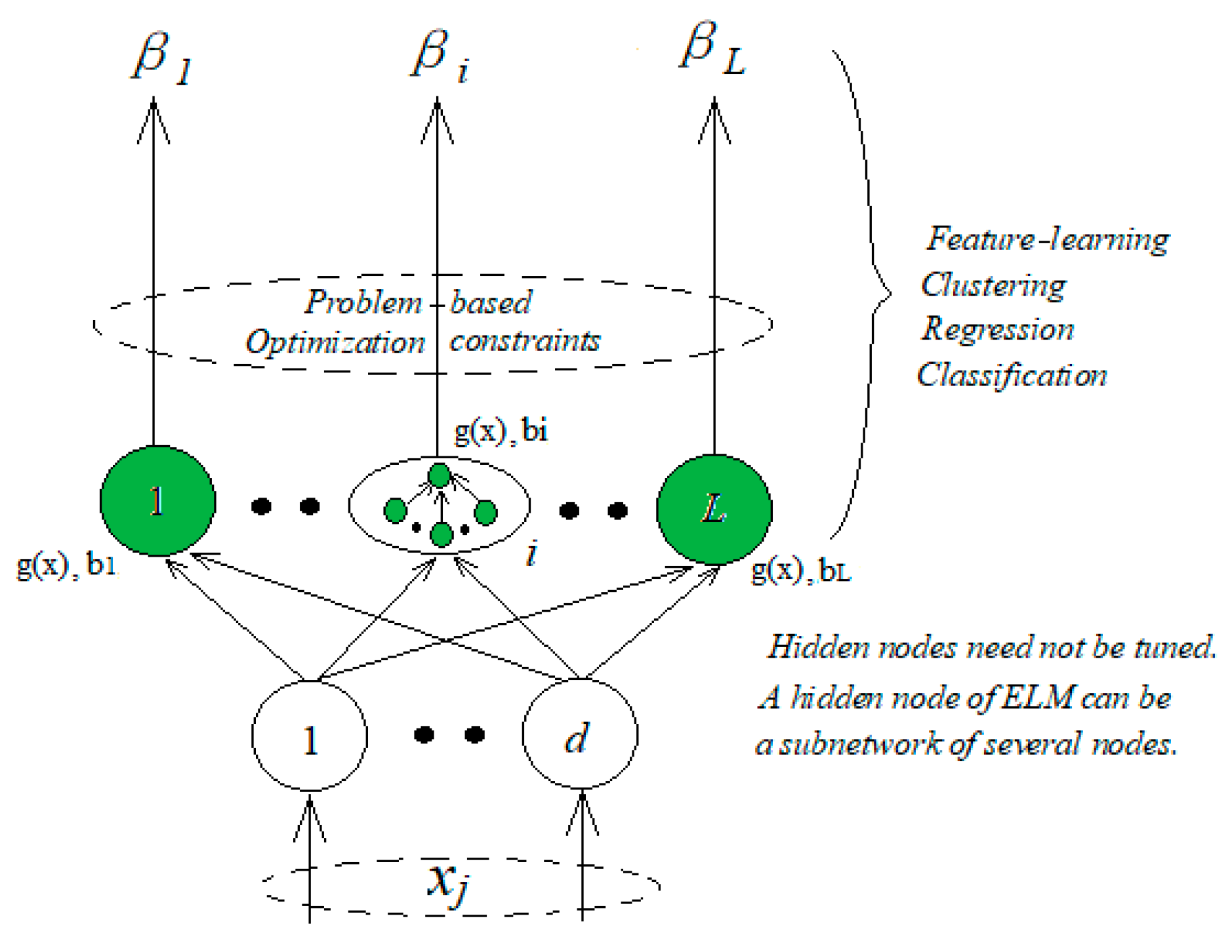
The extreme learning machine (ELM) was developed by Huang et al. in 2004 to introduce machine learning theory [13]. Based on this theory, various related algorithms, including the extreme learning machine with kernel function (KELM), were derived and widely used by researchers in different fields [25,26]. The basic topology of the ELM is shown in Figure 1.

ELM is a generalized single hidden layer feedforward neural network. After randomly generating input weights and offsets, the output weights are obtained through matrix calculation. Compared with the traditional feedforward post-transmission neural network, extreme learning machine has extremely fast training speed, better generalization performance, and easier implementation.

Suppose a given training set N = {(x_i,t_i)|x_i∈R^d, t_i∈R^m, i = 1, 2, …, d}, where x_i is training data, t_i is the category label for each sample. The basic ELM training algorithm can be summarized as follows: (1) randomly assign hidden node parameters: input weight w_i and offset b_i, i = 1, …, L, 1⁄c for bias constant; (2) calculate the hidden layer output matrix H; and (3) obtain an output weight β. Thus,

$$\beta =H^T{\left(\frac{1}{c}+H{H}^T\right)}^{-1}T$$

(17)

Then, the corresponding output function of the ELM is

$$f\left(x\right)=h\left(x\right)\beta =h\left(x\right)H^T{\left(\frac{1}{c}+H{H}^T\right)}^{-1}T$$

(18)

where, h(x) is the hidden layer feature mapping.

ELM guarantees regression prediction accuracy by minimizing output error, which is

$$\underset{L\to \infty }{\lim }\Vert f\left(x\right)-f_o\left(x\right)\Vert =\underset{L\to \infty }{\lim }\Vert {\displaystyle \sum }_{i=1}^L{\beta }_i{h}_i\left(x\right)-f_o\left(x\right)\Vert =0$$

(19)

where f_o(x) is the function to be predicted consisting of the target value.

The basic ELM algorithm has been applied to short-term electric load forecasting [27], high-voltage circuit breaker mechanical fault diagnosis [28], and a tunnel foundation pit deformation intelligent prediction model [29]. ELM demonstrated high quality performance to meet the needs of different applications. ELM is a new algorithm for SLFN, which randomly generates the connection weight between the input layer and the hidden layer, and the threshold of the hidden layer neurons. ELM does not need to be adjusted during the training process; it only needs to set the hidden layer neurons. Therefore, ELM can be used to obtain the only optimal solution. When the number of neurons in the hidden layer is equal to the number of samples in the training set, the ELM can approach all training samples with zero error. However, more neurons in the hidden layer is not necessarily better. From the prediction accuracy of the test set, when the number of neurons in the hidden layer is gradually increased, the prediction rate of the test set gradually decreases. Therefore, it is necessary to comprehensively consider the prediction accuracy of the training set and the test set and make a compromise selection.

Compared to the basic ELM algorithm, the kernel extreme learning machine is more capable of solving regression prediction problems, and faster while obtaining better or similar prediction accuracy [30]. In the KELM algorithm, the specific form of the feature mapping function h(x) of the hidden layer node is not specifically given, but only needs to know the specific form of the kernel function K(u,v) to find the value of the output function. Because the kernel function directly adopts the form of inner product, it is not necessary to set the number of hidden layer nodes when solving the output function, so that the initial weight and offset of the hidden layer do not need to be set.

For the KELM algorithm, a kernel function is introduced to obtain better regression prediction accuracy, as

$$f\left(x\right)=h\left(x\right)H^T{\left[\frac{1}{c}+H{H}^T\right]}^{-1}T=\left[\begin{array}{c}K\left(x,x_1\right)\\ ⋮\\ K\left(x,x_N\right)\end{array}\right]{\left[\frac{1}{c}+{\Omega }_{ELM}\right]}^{-1}T$$

(20)

$${\Omega }_{ELM\left(i,j\right)}=h\left(x_i\right)·h\left(x_j\right)=K\left(x_i,x_j\right)$$

(21)

where Ω_ELM is kernel function matrix, K(u, v) is the kernel function, which usually chooses Gaussian kernel function, and N is the input layer dimension.

Therefore, through the above analysis, we chose KELM to study the DG location and capacity planning in distribution network.

The model mainly uses KELM’s approximation ability of nonlinearity and generalization performance, to approximate the nonlinear relationship expressed with physical model between nodes in power system. In this paper, KELM is used to approximate the relationship between different access points of DG and the change of output power and network node voltage. Through training and testing, the variation of node voltage distribution with the DG access position and output power is given. By judging the root mean square error (RMSE) between the predicted and measured values given by the KELM model, the calculation accuracy of the model is judged. The voltage stability evaluation index is introduced to evaluate the result, so that the DG configuration scheme that satisfies the condition is selected.

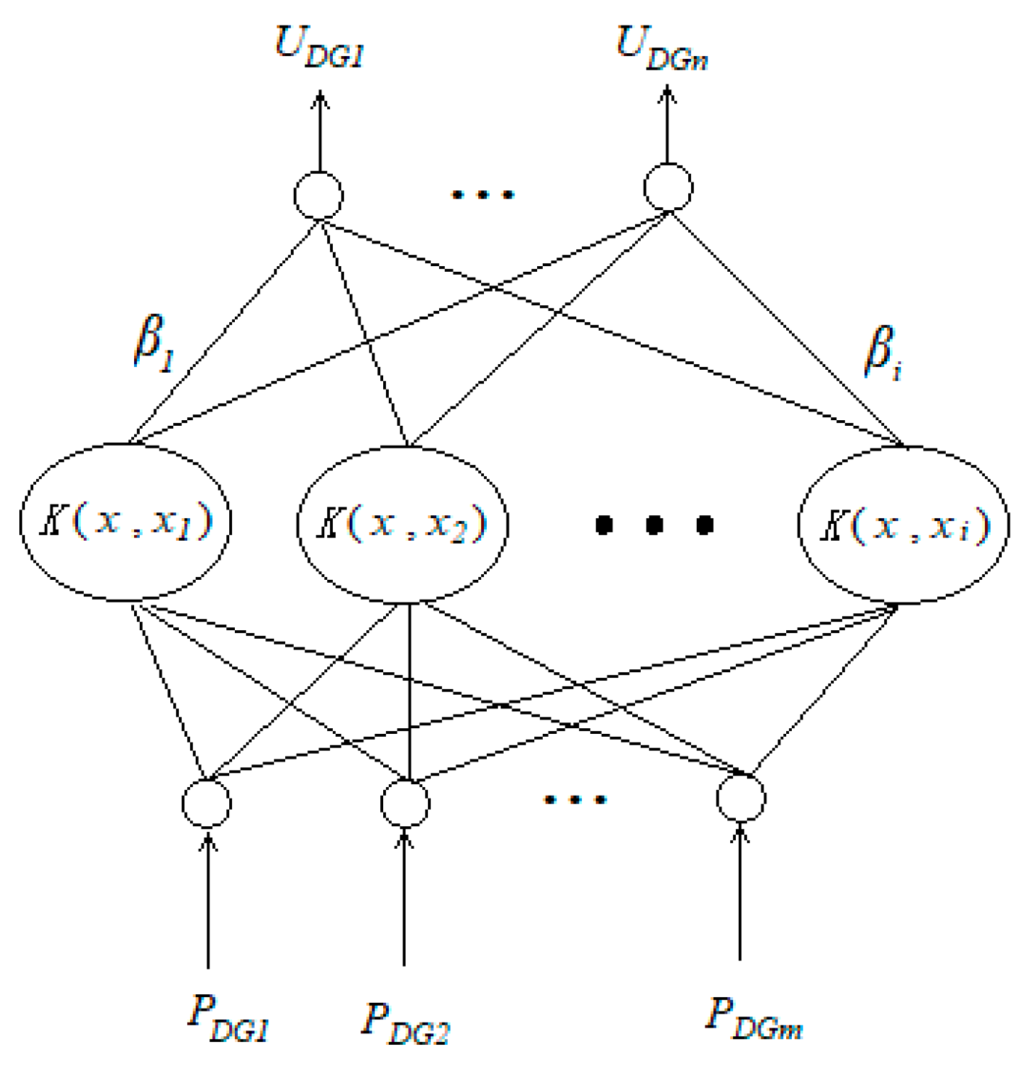
The Figure 2 above shows the structure of the KELM model. P_DG represents the output power of DG, U_DG represents the voltage of the DG access point, and K(u,v) represents the kernel function.

$$\mathrm{RMSE}=\sqrt{\frac{1}{N}{\displaystyle \sum }_{i=1}^N{\left(y\left(i\right)-y^{\ast }\left(i\right)\right)}^2}$$

(22)

In the above formula, RMSE represents the root mean square error, y(i) represents the measured value, y*(i) represents the predicted value given by the KELM model, and N is the number of samples. The smaller the RMSE, the closer the prediction effect is to the measured value.

3.3. Solution Steps

The KELM algorithm is based on data-driven idea with the aim calculating data-driven power flow, and using the KELM algorithm to solve the DG location and capacity selection model. The algorithm is divided into two parts. The first is using the data-driven technology to describe the uncertainty of the wind and photovoltaic power generation output, minimizing the loss of the network as the objective function, and computing power flow that satisfies the constraint conditions. The second is using the obtained results to train KELM to map from DG output to voltage distribution. When the set value of mean square error (RMSE) is satisfied, the DG configuration scheme that meets the requirements is obtained. Finally, the results were evaluated using the voltage stability evaluation index, and the obtained configuration scheme was compared with the existing PSO and GA algorithms.

The solution steps are as follows:

Step 1: Initialize the system parameters, set the type of DG, and obtain basic parameters, such as DG output P_DG.

Step 2: Calculate the power flow of the distribution network without DG to obtain the IVSE index, the voltage profile, and active power loss. Select the point with the highest index value as the initial DG access location.

Step 3: Taking the initial access location as the starting point, calculate the power flow of the distribution network with DG, and record the DG output sequence P_DG and the corresponding node voltage sequence U_DG, as P = {P_DG1, …, P_DGm; U_DG1, …, U_DGn}.

Step 4: The KELM model is trained until the value of the root mean square error (RMSE) satisfies the set value, thereby obtaining the initial configuration scheme of DG, which is the access location and capacity of DG under the basic load condition.

Step 5: Based on the DG configuration scheme obtained in Step 4, the output of the DG is set to vary in the range of 10% to 30% of the total load, recorded as ∆S_DG1 and ∆S_DG2, respectively. Perform the power flow calculation again, and obtain a new data sample, denoted as P’ = {P’_DG1, …, P’_DGm; U’_DG1, …, U’_DGn}.

Step 6: P’ is taken as a test sample and input into the trained KELM. Judge if the RMSE satisfies the set value. If yes, the P’ at this time is saved as the new DG configuration scheme. Otherwise, return to Step 5.

Step 7: From the obtained DG configuration scheme, substitute access capacity and corresponding location information into the pre-return method of distribution network to re-calculate the power flow. Calculate the IVSE index, voltage profile, and active power loss.

Step 8: Select the access capacity and location information of the DG corresponding to the minimum active power loss.

4. Simulations

4.1. Experimental Framework

We used a IEEE33&69-bus radial distribution system for simulation. The original parameters of the system are provided in

Table A1. Data for the IEEE 33-bus radial distribution system.

Node i	Node j	Branch (Ohm)	Load of Node j (kW)
1	2	0.0922 + j0.047	100 + j60
2	3	0.4930 + j0.2511	90 + j40
3	4	0.3660 +j0.1864	120 + j80
4	5	0.3811 + j0.1941	60 + j30
5	6	0.8190 + j0.7070	60 + j20
6	7	0.1872 + j0.6188	200 + j100
7	8	0.7114 + j0.2351	200 + j100
8	9	1.0300 + j0.7400	60 + j20
9	10	1.0440 + j0.7400	60 + j20
10	11	0.1966 + j0.0650	45 + j30
11	12	0.3744 + j0.1238	60 + j35
12	13	1.4680 + j1.1550	60 + j35
13	14	0.5416 + j0.7129	120 + j80
14	15	0.5910 + j0.5260	60 + j10
15	16	0.7463 + j0.5450	60 + j20
16	17	1.2890 + j1.7210	60 + j20
17	18	0.3720 + j0.5740	90 + j40
2	19	0.1640 + j0.1565	90 + j40
19	20	1.5042 + j1.3554	90 + j40
20	21	0.4095 + j0.4784	90 + j40
21	22	0.7089 + j0.9373	90 + j40
3	23	0.4512 + j0.3083	90 + j50
23	24	0.8980 + j0.7091	420 + j200
24	25	0.8960 + j0.7011	420 + j200
6	26	0.2030 + j0.1034	60 + j25
26	27	0.2842 + j0.1447	60 + j25
27	28	1.0590 + j0.9337	60 + j20
28	29	0.8042 + j0.7006	120 + j70
29	30	0.5075 + j0.2585	200 + j600
30	31	0.9744 + j0.9630	150 + j70
31	32	0.3105 + j0.3619	210 + j100
32	33	0.3410 + j0.5362	60 + j40

and

Table A2. Data for the IEEE 69-bus radial distribution system.

Node i	Node j	Branch (Ohm)	Load of Node j (kW)
1	2	0.0050 + j0.0012	0
2	3	0.0050 + j0.0012	0
3	4	0.0015 + j0.0036	0
4	5	0.0251 + j0.0294	0
5	6	0.3660 + j0.1864	2.6 + j2.2
6	7	0.3811 + j0.1941	40.4 + j30
7	8	0.0922 + j0.0470	75 + j54
8	9	0.0493 + j0.0251	30 + j22
9	10	0.8190 + j0.2707	28 + j19
10	11	0.1872 + j0.0691	145 + j104
11	12	0.7114 + j0.2351	145 + j104
12	13	1.0300 + j0.3400	8 + j5.5
13	14	1.0440 + j0.3450	8 + j5.5
14	15	1.0580 + j0.3496	0
15	16	0.1966 + j0.0650	45.5 + j30
16	17	0.3744 + j0.1238	60 + j35
17	18	0.0047 + j0.0016	60 + j35
18	19	0.3276 + j0.1083	0
19	20	0.2106 + j0.0696	1 + j0.6
20	21	0.3416 + j0.1129	114 + j81
21	22	0.0140 + j0.0046	5.3 + j3.5
22	23	0.1591 + j0.0526	0
23	24	0.3463 + j0.1145	28 + j20
24	25	0.7488 + j0.2457	0
25	26	0.3089 + j0.1021	14 + j10
26	27	0.1732 + j0.0572	14 + j10
3	28	0.0044 + j0.0108	26 + j18.6
28	29	0.0640 + j0.1565	26 + j18.6
29	30	0.3978 + j0.1315	0
30	31	0.0702 + j0.0232	0
31	32	0.3510 + j0.1160	0
32	33	0.8390 + j0.2816	14 + j10
33	34	1.7080 + j0.5646	19.5 + j14
34	35	1.4740 + j0.4873	6 + j4
3	59	0.0044 + j0.0108	26 + j18.55
59	60	0.0640 + j0.1565	26 + j18.55
60	61	0.1053 + j0.1230	0
61	62	0.0304 + j0.0355	24 + j17
62	63	0.0018 + j0.0021	24 + j17
63	64	0.7283 + j0.8509	1.2 + j1
64	65	0.3100 + j0.3623	0
65	66	0.0410 + j0.0478	6 + j4.3
66	67	0.0092 + j0.0116	0
67	68	0.1089 + j0.1373	39.22 + j26.3
68	69	0.0009 + j0.0012	39.22 + j26.3
4	36	0.0034 + j0.0084	0
36	37	0.0851 + j0.2083	79 + j56.4
37	38	0.2898 + j0.7091	384.70 + j274.5
38	39	0.0822 + j0.2011	384.70 + j274.5
8	40	0.0928 + j0.0473	40.5 + j28.3
40	41	0.3319 + j0.1114	3.6 + j2.7
9	42	0.1740 + j0.0886	4.35 + j3.5
42	43	0.2030 + j0.1034	26.4 + j19
43	44	0.2842 + j0.1447	24 + j17.2
44	45	0.2813 + j0.1433	0
45	46	1.5900 + j0.5337	0
46	47	0.7837 + j0.2630	0
47	48	0.3042 + j0.1006	100 + j72
48	49	0.3861 + j0.1172	0
49	50	0.5075 + j0.2585	1244 + j888
50	51	0.0974 + j0.0496	32 + j23
51	52	0.1450 + j0.0738	0
52	53	0.7105 + j0.3619	227 + j162
53	54	1.041 + j0.5302	59 + j42
11	55	0.2012 + j0.0611	18 + j13
55	56	0.0047 + j0.0014	18 + j13
12	57	0.7394 + j0.2444	28 + j20
57	58	0.0047 + j0.0016	28 + j20

of the Appendix A. The initial access locations of photovoltaic and wind power generation were determined according to the IVSE index. First, the point with the largest index was selected, and then the lowest point of the node voltage was selected. Using the measured data of wind farms and photovoltaic stations in a project, and adopting data-driven technology, a large number of simulations were carried out to obtain the distribution function and its parameters. According to the simulation results, the wind speed obeyed the Weibull distribution of k = 5.8 and c = 16, and the fan had rated speed v_n of 15 m/s, cut-in speed v_i of 4 m/s, and cut-out speed v_o of 25 m/s. The illumination intensity followed a Weibull distribution with a k = 0.45 and c = 9.18. The number of data sampling times was set to 6000. We assumed that sufficient reactive power was given in the network, and the target of DG was designed and fixed with the aim of minimizing the active power loss. Figure 3 and Figure 4 give out the topology of IEEE33&69-bus radial distribution system, respectively.

4.2. Data Analysis

4.2.1. Results of KELM

After a certain amount of simulation, the configuration schemes of various types of DGs satisfying the restrictions were obtained. Three representative nodes were selected that corresponded to the worst voltage stability point, the lowest voltage amplitude, and any node in the net.

Table 1. Configuration scheme of IEEE 33-bus radial distribution system with DGs.

Node	C1M1	C1M2	C2M1	C2M2	C3M1	C3M2
Node 5	PV	Wind	PV	Wind	Wind	PV
Node 17	-	-	Wind	PV	Wind	Wind
Node 27	-	-	-	-	PV	PV

and

Table 2. Configuration scheme of IEEE 69-bus radial distribution system with DGs.

Node	C1M1	C1M2	C2M1	C2M2	C3M1	C3M2
Node 6	-	-	-	-	PV	Wind
Node 45	PV	Wind	PV	Wind	PV	PV
Node 53	-	-	PV	PV	PV	PV

show the configuration scheme of the IEEE33&69 node system and DG access. Their notation is provided in the following format: in CXMX, C is the abbreviation for Case, the subsequent digit represents the number of DG access, M is the abbreviation of Mode, and the subsequent digit represents the grouping of different types of DG. The CXMXs in Table 1 and Table 2 are different.

Table 1 and Table 2 shows the configuration results of the various types of DGs calculated using the data-driven KELM method. The unit of data in the table is MW.

Table 3. DG location and capacity selection results of IEEE 33-bus radial distribution system (P_loss: active power loss).

Node &Capacity &Ploss	C1M1	C1M2	C2M1	C2M2	C3M1	C3M2
Node 5	1.087	3.427	0.99	3.434	3.524	1.053
Node 17			3.447	1.04	3.474	3.467
Node 27					1.052	1.014
DG (MW)	1.087	3.427	4.437	4.474	8.05	5.534
Ploss (kW)	133.78	119.09	142.63	119.64	171.72	104.14

and

Table 4. DG location and capacity selection results of IEEE 69-bus radial distribution system (P_loss: active power loss).

Node &Capacity &Ploss	C1M1	C1M2	C2M1	C2M2	C3M1	C3M2
Node 6					1.079	3.41
Node 45	0.989	3.418	1.251	3.414	1.058	1
Node 53			2.327	1.06	0.989	0.996
DG (MW)	0.989	3.418	3.578	4.474	3.126	5.406
Ploss (kW)	123.39	124.1	101.35	154.5	92.64	133.45

show the location and capacity (MW) of each type of DG access, and the corresponding active power loss (kW). Among them, the active power loss of the IEEE33&69-bus radial distribution system was 202.45 kW, and 226.5 kW when DG was not connected. It can be seen from Table 3 and Table 4 that the DG access was generally enabled reducing the active power loss of the network. Different access locations and capacities had different degrees of influence on the active power loss of the network.

For the IEEE33-bus radial distribution system, when the DG adopted the C3M2 mode, the active power loss was the least, only 104.14 kW, and the total capacity of the DG access reached 5.534 MW. For the IEEE69-bus radial distribution system, when the DG adopted the C3M1 mode, the active power loss was the least at only 92.64 kW. The total capacity of DG access reached 3.126 MW.

Different access locations had a large impact on active power loss. When accessing a DG, for an IEEE33-bus radial distribution system (33-node), when accessing only node 5, the wind access capacity was higher than PV and the active power loss was lower. For the 69-node system, when only accessing node 45, wind access capacity was higher than PV, but the active power loss was basically the same. When the two DGs were connected for the 33-node system, when the wind access node 5 and the PV access node 17 were swapped, the active loss was lower and the access capacity was larger. For the 69-node system, the active power loss was higher when wind and PV accessed both nodes 45 and 53 at the same time compared to when the wind accessed node 45 or the PV accessed node 53, but the access capacity was larger. Then, when DG accessed three points and when wind replaced the PV access location, the active power loss was higher but the access capacity was also larger.

4.2.2. Voltage Profile

The voltage profile curves of the IEEE33&69 systems before and after DG access are shown in Figure 5 and Figure 6. V__noDG indicates that the DG is not connected, and CXMX represents different DG access modes. The specific allocation is shown in Table 1 and Table 2.

Different access modes had different effects on the voltage profile. For the 33-node system, the network voltage level increased the most in mode C3M1. For the 69-node system, the voltage profile varied with DG in different access modes, with varying degrees of improvement, especially for access points and their nearby nodes. In mode C3M2, the voltage level near the power supply side increased the most. In mode C2M2, the voltage level at the end of the network increased the most.

Overall, as the number of DG accesses increased, the network voltage level improved considerably. In particular, the DG access location had an important impact on the network voltage profile.

The voltage profile of the DG access node in different access modes is shown in Figure 7 and Figure 8. V_noDG indicates the voltage of the corresponding node when the DG is not connected. As can be seen from Figure 7 and Figure 8, the voltage of the access node increased with the access of the DG, and changed with the various DG access modes. For the 33-node system in the case of C3M1, the voltage amplitude of the DG access point was the highest, and C1M2 was the second-highest. For the 69-node system in the case of C2M2, the voltage amplitude of the DG access point was the highest, and C1M2 was the second-highest.

It can be seen from Figure 7 and Figure 8 that different configurations of wind power and PV had different influences on the voltage level of the access point, and the overall trend was to increase the voltage level of the access point. However, the change in access type and access capacity of DG greatly influenced the increase of voltage, and specific analysis is needed.

4.2.3. IVSE Index

For further verification, the DG location and capacity results produced by the KELM method were substituted into the pre-pushback method for power flow calculation, and the IVSE index change rate of the access point was obtained, as shown in Figure 9 and Figure 10. The distribution of the IVSE index change rates for different access modes is shown in Figure 9 and Figure 10. As can be seen in the figure, in the IEEE 33-bus radial distribution system, the index change rate was the highest in the C3M1, and C1M2 was second. In the IEEE 69-bus radial distribution system, the index change rate was the highest in mode C2M2, and C1M2 was second. Note that for the 33-node system, the voltage increase in the DG access point was the largest in C3M1. For the 69-node system, the voltage increase in the DG access point was the largest in mode C2M2.

Comparing the above two examples for different network structures, the increase in the voltage level was related to the number of DGs, and the access type and location, and they are a set of mutually influential factors. In particular, the access location of wind power had a large impact on the voltage profile and had a large access capacity.

Therefore, from the above analysis of the voltage profile and IVSE index changes, the DG location and capacity selection results produced by the KELM algorithm were generally satisfactory and feasible.

4.3. Comparison

Table 5. Comparison of distributed generation (DG) location and capacity selection results for the 33-node system. GA: genetic algorithm; KELM: kernel extreme learning machine; PSO: particle swarm optimization.

References	Methods Used	Number of DGs	Selected Buses	Size of DGs (MW)		Active Power Loss (kW)
Base case	-	-	-	-		202.45
Ref. [32]	PSO	1	7	3.6239	3.6239	131.85
Ref. [33]	PSO	2	29	1.867	1.483	116.71
			31		0.384
Ref. [34]	GA	3	10	3.1	1.5	106.3
			28		0.43
			30		1.07
Proposed	KELM	1	5	3.4	3.4	118.11
		2	5	4.44	3.391	118.4
			17		1.049
		3	5	5.526	1.05	104.2
			17		3.57
			27		0.906

and

Table 6. Comparison of DG location and capacity selection results for 69-node system.

References	Methods Used	Number of DGs	Selected Buses	Size of DGs (MW)		Active Power Loss (kW)
Base case	-	-	-	-		226.5
Ref. [32]	PSO	1	50	3.685	3.685	87.63
		2	37	3.526	1.314	86.68
			50		2.212
Ref. [34]	GA	3	21	2.99	0.93	90.3
			51		1.075
			53		0.985
Proposed	KELM	1	45	3.42	3.418	124.1
		2	45	3.58	1.251	101.3
			53		2.327
		3	6	3.126	1.079	92.6
			45		1.058
			53		0.989

compare the results produced by the KELM algorithm with the PSO and GA methods from the aspects of DG access number, access location, access capacity, and active power loss. Table 5 corresponds to IEEE 33-bus radial distribution system (referred to as the 33-node system) and Table 6 corresponds to the IEEE 69-bus radial distribution system (referred to as the 69-node system).

It can be seen from Table 5 and Table 6 that the results obtained by the KELM method and PSO and GA algorithms were similar.

For the 33-node system, when the DG was connected to one position, the DG access capacity was similar to the other methods, and the configuration active power loss given by KELM was lower. When the DG was connected to two, the DG access capacity produced by KELM was higher than that by the PSO algorithm, and the active loss was similar. When the DG was connected to three, the DG access capacity given by KELM was higher than that of the GA algorithm, and the active power loss was lower.

For the 69-node system, when the DG was connected to one position, the DG access capacity was similar to the other methods, and the configuration active power loss produced by KELM was slightly higher. When DG was connected to two, the DG access capacity given by KELM was similar, and the active loss was a little higher than the PSO algorithm, but still lower than the active power loss when the DG was not connected. When the DG was connected to three, the DG access capacity produced by the KELM was higher than that of the GA algorithm, and the active power loss was similar.

Based on the above comparison, the proposed KELM method provides effective and feasible DG configuration results. When the target of minimum active power loss was used, the various DG configuration schemes produced by the KELM method were better than the existing algorithms, with larger capacity and lower or similar power loss.

5. Discussion

Through the above simulation experiments and comparative analysis, the access of DG generally improved the network voltage level, reduced the active power loss, and changed the access location of different types of DG, which had different effects on the network voltage level.

The access of the DG not only improved the access node, but also increased the voltage level of the nodes near the access point. Compared with photovoltaic, wind power had a larger access capacity and increased the network voltage level more. Through statistical analysis of the simulation data, the average degree of voltage increase by DG access was about 6%. The access type, access location, and capacity of the DG produced different changes in the network’s active power loss. Due to the large capacity of wind power, the degree of impact on the network’s active power loss was greater. When wind power and photovoltaic were simultaneously connected, the calculation of the KELM method provided various DG configuration schemes that were more helpful to reduce network loss. With further increase in the number of DG accesses, higher access capacity was achieved through KELM calculation, and the capacity increase averaged about 4%.

The rate of change in the IVSE index represents the change in the network voltage profile before and after DG access. Through this index, the influence of different configuration schemes of DG on the network voltage profile was further verified. Notably, the influence on the access node had a greater impact.

In addition, the DG configuration results obtained by the KELM were compared with the existing PSO and GA methods. The comparison results showed that the results produced by the KELM algorithm were effective and feasible, and could meet the actual needs of the project. In terms of calculation time, according to the existing research, when the machines used are all ordinary laptops, and the calculation speed and memory of the CPU are basically the same, the calculation time of PSO and its improved algorithm (such as quantum-behaved PSO and improved quantum-behaved PSO) were published by Peng, X.G. et al. [35] as 719.6 s, 538.3 s, and 419.2 s, respectively. The average calculation time of SVM is 870.4s. While that of KELM is 324.7 s. Explain that KELM is fast. Existing optimization algorithms, such as PSO and GA, need to constantly adjust relevant parameters and set various search strategies by iteratively updating to avoid falling into local minimum values and improving the optimization effect. The KELM algorithm introduces the kernel function into the extreme learning machine and replaces the random mapping in the basic ELM with kernel mapping, which effectively improved the generalization ability and stability problems caused by the random set of the hidden layer parameters. The complexity of the calculation was greatly reduced and avoids the setting of the number of hidden layer nodes. The iterative adjustment is not needed, and the least square optimization solution can be obtained. Therefore, the KELM algorithm requires less human intervention and has a faster training speed. The network parameter adjustment process is simple, consumes less time, and has better stability and greater generalization ability.

On the other hand, in order to prove the prediction accuracy of the proposed method, the KELM method is compared with SVM, the root mean square error is used as the evaluation index, and the comparison results are given. When maintaining the same basic conditions, the RMSE of KELM is approximately 0.000491 and the RMSE of SVM is approximately 0.1042. The prediction accuracy of KELM is higher than SVM.

6. Conclusions

We used data-driven technology to describe the uncertainty of wind and photovoltaic power generation and introduced this technology into the power flow calculation of distribution network with multi-types of DG. By training KELM, the mapping of various DG output to node voltage profile is realized. Under the condition of ensuring the minimum network loss, a configuration scheme that satisfies the constraints of network security operation is given. Voltage stability evaluation indexes were introduced to evaluate the DG location and capacity selection results. The IEEE33&69-bus radial distribution system is used as an example to simulate, and the configuration results of DG are compared with the existing PSO and GA algorithms to verify the effectiveness and feasibility of the proposed method. In addition, the calculation time and prediction accuracy are compared with the SVM algorithm, which verifies that the proposed method has faster calculation speed and better prediction accuracy.

Therefore, the conclusions of this paper are briefly summarized as follows:

(1)

DG access improves the network voltage level, especially the access of large-capacity wind power. By adopting the method proposed in this paper, the configuration scheme increases voltage amplitude by an average of 6%.

(2)

DG access reduces network loss. With the increase in the number of DG accesses, higher access capacity can be achieved by adopting the method proposed in this paper, and the capacity increase averages about 4%.

(3)

Through comparison of the existing PSO and GA methods, the effectiveness, feasibility, calculation speed, and high precision of the proposed method were verified.

(4)

Using this method, detailed configuration schemes of various types of DGs can be obtained. Combined with the fast calculation speed, the online operation control schemes of distribution networks with a high proportion of distributed power access can be considered.

As we only addressed the wind and photovoltaic power generation problems for the location and capacity selection of a distribution network, our study has limitations. In the future, with the development of technology, it is necessary to consider the access of new elements to the distribution network, such as electric vehicles and energy storage devices, to constitute a multi-energy interconnect system. These additional connections will change the basic characteristics of the distribution network, so further research needs to be completed to determine how to use the data-driven KELM method on coordinated control and optimization of multi-energy systems.

References

1. Mahmoud Pesaran, H.A.; Huy, P.D.; Ramachandaramurthy, V.K. A review of the optimal allocation of distributed generation: Objectives, constraints, methods, and algorithms. Renew. Sustain. Energy Rev. 2017, 75, 293–312. [Google Scholar] [CrossRef]
2. Ehsan, A.; Yang, Q. Optimal integration and planning of renewable distributed generation in the power distribution networks: A review of analytical technique. Appl. Energy 2018, 210, 44–59. [Google Scholar] [CrossRef]
3. Vita, V.; Alimardan, T.; Ekonomou, L. The impact of distributed generation in the distribution networks’ voltage profile and energy losses. In Proceedings of the 9th IEEE European Modelling Symposium on Mathematical Modelling and Computer Simulation, Madrid, Spain, 6–8 October 2015; pp. 260–265. [Google Scholar]
4. Vita, V. Development of a decision-making algorithm for the optimum size and placement of distributed generation units in distribution networks. Energies 2017, 10, 1433. [Google Scholar] [CrossRef]
5. Asimakopoulou, G.E.; Hatziargyriou, N.D. Evaluation of Economic Benefits of DER Aggregation. IEEE Trans. Sustain. Energy 2018, 9, 499–510. [Google Scholar] [CrossRef]
6. Baghayipour, M.R.; Hajizadeh, A.; Shahirinia, A.; Chen, Z. Dynamic Placement Analysis of Wind Power Generation Units in Distribution Power Systems. Energies 2018, 11, 2326. [Google Scholar] [CrossRef]
7. Li, M.; Xue, F.; Shi, J.; Qin, Z.; Ling, L.; Yang, T. Tri-level Coordinated Planning Model of Distributed Generator and Intelligent Soft Open Point for Active Distributed Network. Autom. Electr. Power Syst. 2018, 42, 86–93. [Google Scholar]
8. Wang, L. Locating and Sizing of Distributed Generations in Distributed Network Considering Uncertainties. Distrib. Energy 2018, 42, 86–93. [Google Scholar]
9. Chao, Q.; Dong, X.; Jiang, T. Optimization Planning of Integrated Electricity-Gas Community Energy System Based on Coupled CCHP. Power Syst. Technol. 2018, 42, 2456–2466. [Google Scholar]
10. Li, P.; Zeng, X.; Li, X.; Hu, Z.; Ke, F.; Tan, Z. Unified Equivalent Modeling of Distributed Generation Using Artificial Neural Network and Its Application in PSASP. Power Syst. Technol. 2016, 40, 1224–1230. [Google Scholar]
11. Fu, Y.; Liu, Y.; Huang, L.; Wei, S.; Liu, L. Optimization of Grid Integration Network for Offshore Wind Farm Cluster. Proc. CSEE 2018, 38, 3441–3450. [Google Scholar]
12. Zhu, J.; Gu, W.; Zhang, H.; Wang, W.; Zhu, G.; You, D. Optimal Siting and Sizing of Distributed Generators Considering Dynamic Network Reconfiguration. Autom. Electr. Power Syst. 2018, 42, 111–119. [Google Scholar]
13. Huang, G.B.; Zhu, Q.Y.; Siew, C.K. Extreme learning machine: Theory and applications. Neurocomputing 2006, 70, 489–501. [Google Scholar] [CrossRef] [Green Version]
14. Ren, R.; Li, J. Optimizing Kernel Extreme Learning Machine for Medium Electricity Load Forecasting. Meas. Control Technol. 2018, 37, 15–19. [Google Scholar]
15. Shen, K.; Ren, X.; Wang, X.; Ma, F. The Buried Cutting Process Data-Driven Model Based on Extreme Learning Machine. Equip. Manuf. Technol. 2017, 6, 1–7. [Google Scholar]
16. Zhang, Z.; Li, G.; Wei, J. Probabilistic evaluation of voltage quality in distribution networks considering the stochastic characteristic of distributed generators. Proc. CSEE 2013, 33, 150–156. [Google Scholar]
17. Evangelopoulos, V.A.; Georgilakis, P.S. Optimal distributed generation placement under uncertainties based on point estimate method embedded genetic algorithm. IET Gener. Transm. Distrib. 2014, 8, 389–400. [Google Scholar] [CrossRef]
18. Jiang, B.; Wu, J.; Feng, L.; Wu, K.; Liang, R.; Yang, B.; Li, X.; Chen, H. Research on static voltage stability calculation indicator of active distribution network with distributed generation. J. Electron. Meas. Instrum. 2017, 31, 885–891. [Google Scholar]
19. Tu, J.; Yin, Z.; Xu, Y. Study on the Evaluation Indicator System and Evaluation Method of Voltage Stability of Distribution Network with High DG Penetration. Energies 2018, 11, 79. [Google Scholar]
20. Fan, S.; Ai, Q.; He, X. Risk Analysis on Dispatch of Virtual Power Plant Based on Chance Constrained Programming. Proc. CSEE 2015, 35, 4025–4034. [Google Scholar]
21. Xue, Y.; Lai, Y. Integration of macro energy thinking and big data thinking: Part one big data and power big data. Autom. Electr. Power Syst. 2016, 40, 1–8. [Google Scholar]
22. Xue, Y.; Lai, Y. Integration of macro energy thinking and big data thinking: Part two applications and explorations. Autom. Electr. Power Syst. 2016, 40, 1–13. [Google Scholar]
23. Chi, R.; Hou, Z.; Huang, B. Optimal iterative learning control of batch processes: From model-based to data-driven. Acta Autom. Sin. 2017, 43, 917–932. [Google Scholar]
24. Chen, L. Data driven product management. IEEE Eng. Manag. Rev. 2018, 46, 16–18. [Google Scholar]
25. Lyu, H.; Xia, H.; Ma, X.; Zhao, J.; Chen, Y. Research on data-driven industrial Internet solutions. J. Xi’an Univ. Posts Telecommun. 2018, 23, 104–110. [Google Scholar]
26. Xu, D.; Deng, J.; Yan, W.; Ji, Z. Novel data-driven path tracking constrained control for intelligent vehicle autonomous overtaking system. Control Theory Appl. 2018, 35, 283–290. [Google Scholar]
27. Dong, H.; Li, M.; Zhang, S.; Han, L.; Li, J.; Su, X. Short-term power load forecasting based on kernel principal component analysis and extreme learning machine. J. Electron. Meas. Instrum. 2018, 32, 188–193. [Google Scholar]
28. Huang, N.; Chen, H.; Lin, L.; Qi, J. Mechanical Fault Diagnosis of High Voltage Circuit Breakers Based on S-transform and Extreme Learning Machine. High Volt. Appar. 2018, 54, 74–80. [Google Scholar]
29. Chen, Y. Application of Intelligent Algorithm Based on Genetic Algorithm and Extreme Learning Machine to Deformation Prediction of Foundation Pit. Tunn. Constr. 2018, 38, 941–947. [Google Scholar]
30. Huang, G.B.; Bai, Z.; Kasun, L.L.C.; Vong, C.M. Local receptive fields based extreme learning machine. IEEE Comput. Intell. Mag. 2015, 10, 18–29. [Google Scholar] [CrossRef]
31. Baran, M.E.; Wu, F.F. Optimal sizing of capacitors placed on a radial distribution system. IEEE Trans. Power Deliv. 1989, 4, 735–743. [Google Scholar] [CrossRef]
32. Aman, M.M.; Jasmon, G.B.; Bakar, A.H.A.; Mokhlis, H. A new approach for optimum simultaneous multi-DG distributed generation units placement and sizing based on maximization of system loadability using HPSO (hybrid particle swarm optimal) algorithm. Energy 2014, 66, 202–215. [Google Scholar] [CrossRef]
33. Jamian, J.J.; Mustafa, M.W.; Mokhlis, H. Optimal multiple distributed generation output through rank evolutionary particle swarm optimization. Neurocomputing 2015, 152, 190–198. [Google Scholar] [CrossRef]
34. Moradi, M.H.; Tousi, S.M.R.; Abedini, M. Multi-objective PFDE algorithm for solving the optimal siting and sizing problem of multiple DG sources. Int. J. Electr. Power Energy Syst. 2014, 56, 117–126. [Google Scholar] [CrossRef]
35. Peng, X.G.; Lin, L.X.; Liu, Y.; Wang, X.H.; Meng, A.B. Optimal Distributed Generator Allocation Method Based on Correlation Latin Hypercube Sampling Monte Carlo Simulation Embedded Crisscross Optimization Algorithm. Proc. CSEE 2015, 35, 4077–4085. [Google Scholar]
Figure 1. Basic topology of extreme learning machine (ELM). βi is the output weight, xj is the input training data, d is the number of input layer units, L is the number of hidden layer nodes, and g(x) is the output function of hidden layer nodes.
Energies 12 00109 g001
Figure 2. KELM Structure diagram.
Energies 12 00109 g002
Figure 3. IEEE 33-bus radial distribution system topology [31].
Energies 12 00109 g003
Figure 4. IEEE 69-bus radial distribution system topology [31].
Energies 12 00109 g004
Figure 5. Voltage profile of IEEE33-bus radial distribution system with various types of DG. V_noDG indicates that the DG is not connected.
Energies 12 00109 g005
Figure 6. Voltage profile of IEEE69-bus radial distribution system with various types of DG. V_noDG indicates that the DG is not connected.
Energies 12 00109 g006
Figure 7. IEEE 33-bus radial distribution system voltage profile of access nodes with different access modes.
Energies 12 00109 g007
Figure 8. IEEE 69-bus radial distribution system voltage profile of access nodes with different access modes.
Energies 12 00109 g008
Figure 9. IEEE 33-bus radial distribution system IVSE index change rate of access nodes in different access modes.
Energies 12 00109 g009
Figure 10. IEEE 69-bus radial distribution system IVSE index change rate of access nodes in different access modes.
Energies 12 00109 g010