Joint Optimal Policy for Subsidy on Electric Vehicles and Infrastructure Construction in Highway Network

Abstract

The promotion of the battery electric vehicle has become a worldwide problem for governments due to its short endurance range and slow charging rate. Besides an appropriate network of charging facilities, a subsidy has proved to be an effective way to increase the market share of battery electric vehicles. In this paper, we investigate the joint optimal policy for a subsidy on electric vehicles and infrastructure construction in a highway network, where the impact of siting and sizing of fast charging stations and the impact of subsidy on the potential electric vehicle flows is considered. A new specified local search (LS)-based algorithm is developed to maximize the overall number of available battery electric vehicles in the network, which can get provide better solutions in most situations when compared with existed algorithms. Moreover, we firstly combined the existing algorithms to establish a multi-stage optimization method, which can obtain better solutions than all existed algorithms. A practical case from the highway network in Hunan, China, is studied to analyze the factors that impact the choice of subsidy and the deployment of charging stations. The results prove that the joint policy for subsidy and infrastructure construction can be effectively improved with the optimization model and the algorithms we developed. The managerial analysis indicates that the improvement on the capacity of charging facility can increase the proportion of construction fees in the total budget, while the improvement in the endurance range of battery electric vehicles is more efficient in expanding battery electric vehicle adoption in the highway network. A more detailed formulation of the battery electric vehicle flow demand and equilibrium situation will be studied in the future.

1. Introduction

Battery electric vehicles (BEVs) are regarded as a most promising solution to increasingly serious air pollution and global warming [1]. The widely adoption of BEV can bring many advantages, such as energy conservation, emission reduction and clean energy application [2,3]. However, the popularization of BEVs is a universal difficulty for the governments worldwide. Compared with traditional internal combustion engine (IDE) vehicles at the same price, the endurance range of BEVs is much shorter [4]. The adoption of BEVs in a highway network relies on a widespread network of charging facilities. On the other hand, customers are reductant to purchase BEVs due to the long recharging time, even though there may be sufficient charging facilities. Thus, besides constructing basic infrastructures, governments need to increase the ownership of BEVs among citizens.

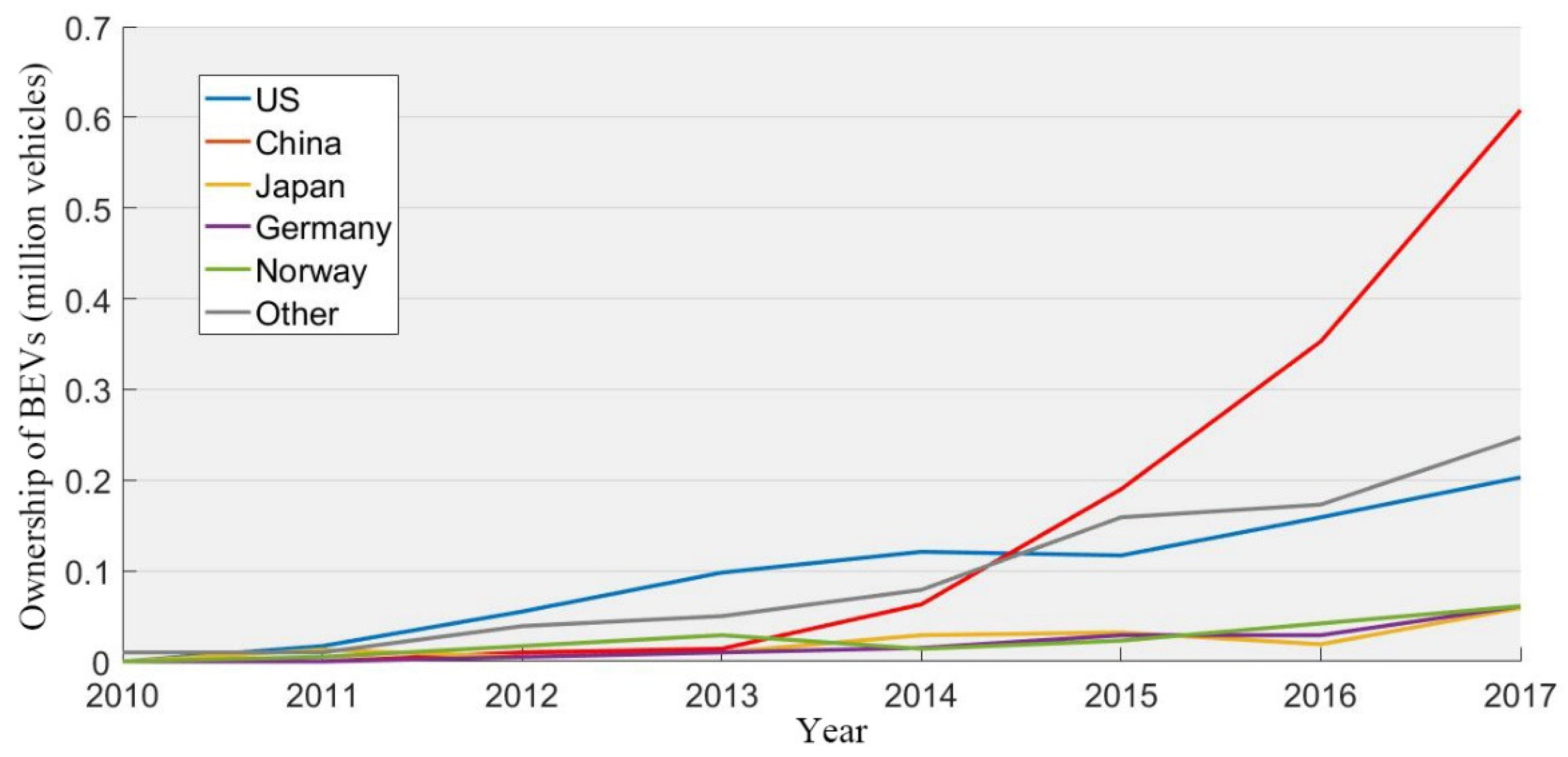
To promote BEV purchasing, some governments provide a subsidy to the customers who own or buy BEVs, such as in China and India. According to the data of EV-volumes [5] in Figure 1, since the Chinese government began to largely implement the subsidy in 2013 [6], the ownerships of BEVs has gained huge growth, which is much faster than in other countries. China now has the largest market share in the world. This proves that the subsidy is an effective way to increase the willing of customer to purchase BEVs.

On the other hand, the location and size of a charging station is essential for the BEVs running on the highway network. As the endurance range of a BEV is much shorter [7], it needs to recharge more frequently than IDE vehicles. Meanwhile, even with a fast charging pile, it still takes about half an hour to take a fully recharge for BEV, which means the service capacity of a charging pile is limited. As the construction and maintenance cost of the charging facility is high, the investment is often not sufficient to cover all the charging demand. To maximize the BEV traffic on the highway network, an optimal siting and sizing scheme of the charging station is necessary to take full use of the investment. Meanwhile, as the total investment is limited, the policymaker needs to balance the budget distribution on the facility construction and the subsidy.

The siting and sizing problem of a charging station is different from the traditional facility location problem, which can be described in four aspects: (1) instead of concentrating in some nodes, the demand in the problem is more like a flow from one node to another; (2) The flow demand often needs to recharge multiple times and the distances between the recharging nodes cannot exceed a fixed length that is called the endurance constraint; (3) The volume of the demand that can be charged depends on the service capacity of the charging stations on the route; (4) The drivers have their own strategy to choose the station when there are multiple choices. In recent years, much research has investigated the siting and sizing problem of charging station, which is introduced as follows.

For facilities like advertisements, demand is more like being captured instead of fulfilled by the facility. To formulate the location problem of these facilities, Hodgson [8] presents a new model called the flow capturing location model (FCLM), in which the demand is presented as a flow from origin to destination (O–D). Once a demand flow passes through a facility, the demand is marked captured by the facility. Alhough there is no passing limit in FCLM, it is the basic model of many problems with flow demand. Kuby and Lim [3] add the endurance constraint into the FCLM, which makes it applicable to solve the location problem of a refueling station. They define that a demand can proceed only if there are sufficient stations at fixed distances along the path. The extended model is called a flow refueling location model (FRLM). A practical case of road network in Florida is discussed to prove the performance of FRLM [9]. Kuby et al. pointed out that the largest difficulty is controlling the computing complexity from the exponential growth of the combination number. Upchurch and Kuby [10] then compare the performance of FRLM and traditional node-based models. The result proves that FRLM can achieve a better solution in the location problem of a refueling station in a highway network. After that, much research has investigated FRLM. Lin et al. [11] proposed an approach called the “fuel-travel-back” pattern to estimate the potential demand based on FRLM. They suppose that the place where you drive most is the place where you are most likely to refuel. Thus, the origin of a trip can be found with the vehicle miles traveled (VMT). In this way, the demand of a road segment is concentrated into a node, which simplifies the solving process of FRLM. Wang and Lin [12] change the objective of FRLM to minimize the cost for fulfilling all refueling demand. They use the method of “set covering” to solve FRLM by cutting demand into segments, which saves much of the calculating time.

In FRLM, the refueling time is short enough that it can be ignored. However, it is unreasonable for the BEVs as the recharging time is relatively long, which means the service capacity of a charging pile is limited. Upchurch et al. [13] extend the FRLM by adding a capacity constraint to fit the requirement of the charging station location problem, namely, the capacitated flow refueling location model (CFRLM). In CFRLM, the service capacity of a charging station is measured by the number of the charging piles in it. Meanwhile, when the service capacity is limited, the charging strategy of drivers needs to be formulated, as it can impact on the sizing scheme of a charging station. Upchurch et al. assume that the recharging pattern of a driver can be decided by the planner in a system-optimal manner. Besides CFRLM, Capar et al. [14] raise another model to formulate the siting and sizing problem of a charging station called the arc cove-path cover model (AC-PC). The AC-PC is based on the observation that if all the sub-paths of a path are accessible, the path is also accessible. In this way, the demand of a path can be separated to every arc of the path, in which the station choice does not have to be discussed. In other words, AC-PC places some redundancy to fulfill all the possible situations of station choice. Wang et al. [15] find a reasonable approach to formulate the charging strategy of drivers with utility theory. They find that different charging schemes in a path are just like different routes for an O–D pair. The drivers in the path have their own utility to choose every charging scheme depending on the congestion situation of each charging station. Thus, they define the usefulness of a driver to choose a charging scheme by the possibility of being served. However, the algorithm they used only contains optimization in the siting aspect. Once the siting scheme of stations is settled, the sizing scheme is made with some fixed strategy, which will miss better solutions.

There is also some research studying the location problem of charging stations in urban areas. Sadeghi-Barzani et al. [16] investigate the impact of the electric grid loss, development cost, substations location and other aspects on location decision. Andrenacci et al. [17] concentrate on demand with the cluster method, which separates the entire network into subareas. Xiang et al. [18] consider the distribution of charging demand in time periods of both weekdays and weekends. An equilibrium situation is defined to illustrate the system optimization of the road network. Arias et al. [19] estimate the charging patterns of different kinds of BEVs with a Markov chain, with which they can predict the volume of O–D flows with historical traffic data. Zhang et al. [20] prove that placing multiple cables on one charging output can achieve higher efficiency of facilities. As the traveling distance is much shorter in urban area, the studies introduced above do not consider the endurance constraint. The demand is directly linked to the charging facilities, which is more suitable for node-based models.

In this paper, we firstly introduced the joint policy planning problem of the subsidy and the infrastructure construction in adopting BEVs. A specified FRLM is developed to formulate the joint optimization of a subsidy and infrastructure construction under a budget constraint, which contains the subsidy choice and the siting and sizing of charging station. A specified local search (LS) algorithm is approached to maximize the number of charged BEVs under given investment, which allows the optimization in both the siting and sizing aspects. Finally, a practical case study from the highway network of Hunan, China, is proposed to test the effectiveness of the algorithm in solving the deployment problem of the subsidy and the construction fee in total investment.

The rest of this study is structured as follows: Section 2 describes the problem of this subscription and constructs the optimization model. A local search-based algorithm is also introduced. Section 3 presents a practical case study based on the highway network of Hunan, China. The algorithm’s comparison and managerial analysis are also discussed. Section 4 discusses the practical meaning and the limitations of this study. Finally, Section 5 presents the conclusion and future work.

2. Materials and Methods

In this section, we specified the capacitated flow refueling location model (CFRLM) developed in [15] to formulate the joint policy optimization problem of subsidy and infrastructure construction for BEV adoption. The impact of the subsidy is reflected in the amount of potential demand in the road network. As the budget is limited, to maximize the number of charged BEVs in the network, a local search-based algorithm is illustrated to find the optimal siting and sizing scheme of a charging station, which can further improve the solution with two-stage optimization.

2.1. Model Formulation

In this subsection, we formulate the siting and sizing problem of a charging station in a similar way to our prior work [15], which is included in parts (1) and (2). Then the impact of the subsidy is formulated into the problem to make it fit the optimization in this paper, which is illustrated in part (3). Finally, the main optimization model is presented in part (4). The notations used in the model development are described in Nomenclature.

2.1.1. Highway Network Modeling

The highway network is defined as a network G(N, L), where N consists of the O–D nodes and the candidate locations for a charging station, and L denotes the roads between these nodes. The O–D nodes denote the cities and towns in the network while the candidate locations are the existing service areas. Constructing charging stations in the service areas can save budget as there has already been some basic infrastructure. As the charging pile stations are often built in pairs along the road, we combine the twin stations in the same node as one, which can serve the demand from both directions. The service capacity of each station depends on the number of charging piles in it.

The charging demand appears like a flow that comes from one O–D node to another O–D node. The deviation from the shortest path is not considered as it may cause unacceptable distance addition in highway network. The max demand between two O–D nodes is called the potential demand represented by $f_q$, where $q$ represents the path between these two O–D nodes.

The actual number of BEVs that can go through a path depends on many aspects, including the location and size of charging station, congestion situation of the network and the charging strategy of customs. These aspects are discussed in detail in next subsection.

2.1.2. Driver Utility and Equilibrium Situation

When traveling on the road, the BEVs need to recharge every fixed distance to avoid being out of power. This distance is called the endurance range of a BEV. Thus, if there are no sufficient charging stations along the path, the demand of this path cannot be fulfilled at all. Figure 2 gives a simple instance of a highway network in which s, t are O–D nodes and A, B, C are candidate nodes. If the endurance range of BEV is 150 km, there are two station sets {A, C} and {B, C} that can support the demand of path (s, t). These station sets are called the station combinations of path (s, t). However, the combination {A, B, C} is not considered, because no one is willing to spend extra waiting time while there are some better choices.

If there are three stations constructed in node A, B and C, the customers of path (s, t) may have multiple combinations to achieve their trip. As the service capacity of each station is limited, the customers have their own preference to avoid congestion. In this paper, we exploit random utility theory [21] to illustrate the distribution of potential charging demand. The random utility theory was originally used in traffic equilibrium problem, which can measure the utility of drivers to choose one from all the routes of an O–D pair. All the aspects that affect a driver’s willingness are contents in the deterministic component V, which can be observed and measured. Besides, each individual has a random error $\epsilon$ with a mean value of zero. Thus, the utility of a driver n in the path q to choose a combination h can be expressed as follows:

$$U_{qh}^n=V_{qh}^n+{\epsilon }_{qh}^n,\forall h\in H_q,\forall q\in Q$$

(1)

where $U_{qh}^n$ is the utility of driver n in path q to choose combination h, $V_{qh}^n$ is the deterministic component value for the choice of driver n, and ${\epsilon }_{qh}^n$ is an individual random error [15].

In a traffic equilibrium problem, V appears as a function illustrating the equivalent cost of all the aspects. In the problem of this paper, as the route is fixed, the combinations of an O–D pair are treated as the different routes. The only difference between these combinations is the service proportion $P_{qh}$, which is expressed by Equation (2).

$$P_{qh}=E(P_{qh}^n)=\{\begin{array}{ll}\frac{f_{qh}^{\prime }}{f_{qh}},& f_{qh}\ne 0\\ 1,& f_{qh}=0\end{array},\forall q\in Q,\forall h\in H_q$$

(2)

Thus, $P_{qh}^n$ can be treated as the utility of drivers in path q who choose a combination h. In the optimization problem of this paper, we focus on the macroscopic optimization of the policy, so the utility discussed here is the expectation, which can be expressed with Equations (3) [15] and (4):

$$V_{qh}^n=P_{qh}^n$$

(3)

$$U_{qh}=E(U_{qh}^n)=E(V_{qh}^n)+E({\epsilon }_{qh}^n)=P_{qh},\forall q\in Q,\forall h\in H_q$$

(4)

where the mean value of ${\epsilon }_{qh}^n$ is zero.

According to utility theory, drivers always try to obtain maximum utility from routes. When given a siting and sizing scheme of a charging station, the equilibrium situation of potential flow should meet the following restrictions:

Firstly, for a path, the service proportions of its combinations should be equal with each other. If the service proportion of one combination is higher, the drivers who choose other combinations will change their prior choice to achieve higher proportions. This restriction can be expressed with Equation (5) [15]:

$$P_{qh}=P_{q{h}^{\prime }},\forall h,h^{\prime }\in H_q,\forall q\in Q$$

(5)

Secondly, the charging station serves the BEVs from all paths indifferently. The number of BEVs that are charged by a combination depends on the most congested station, which is called the bottleneck of the combination. If the service proportion of station k is Z_k, the definition of a bottleneck is expressed with Equation (6) [15]:

$$P_{qh}\le Z_k,\forall q\in Q,\forall h\in H_q,\forall k\in K_h$$

(6)

According to the second restriction, all the combinations that treat the same station as a bottleneck should have the same service proportion. This can be expressed with Equation (7) [15]:

$$P_{qh}=P_{q^{\prime }{h}^{\prime }},\forall h,h^{\prime }\left|\right\{c_{hk}=c_{h^{\prime }{k}^{\prime }},\forall k\in K_h\cap K_{h^{\prime }}\}$$

(7)

Above all, the equilibrium situation can be described with Equations (2), (5), (6) and (7). To calculate the equilibrium situation of a given siting and sizing scheme, we use the approach based on gradient projection developed in [15]. This approach can be expressed with the following steps:

Initialization: at the beginning, all the potential flows $f_{qh}$ are set with Equation (8), which aims to uniformly separate the potential demand of every path to all the combinations of it.

$$f_{qh}=\frac{f_q}{{\displaystyle \sum _{h\in H}{b}_{qh}}}$$

(8)

Step 1: Sort all the stations with the value of $Z_k$, which is expressed in Equation (9):

$$Z_k=\frac{I{x}_k-{\displaystyle \sum _{q\in Q}{\displaystyle \sum _{h\in H}{a}_{hk}{b}_{qh}{v}_{qh}{f}_{qh}^{\prime }}}}{{\displaystyle \sum _{q\in Q}{\displaystyle \sum _{h\in H}{a}_{hk}{b}_{qh}(1-v_{qh})f_{qh}}}}$$

(9)

where $v_{qh}$ is a recorder, that is 1, which means the $f_{qh}$ has been impacted by a more congested station, and 0 otherwise. For the station with minimum $Z_k$, set all the $f_{qh}^{\prime }$ that are charged by station k with Equation (10), and then mark the corresponding $v_{qh}$ as 1. This process is repeated until all the $Z_k$ is no less than 1.

$$f_{qh}^{\prime }=Z_k{f}_{qh}$$

(10)

Step 2: For all the combinations that can charge the path $q\in Q$, calculate the difference of $P_{qh}$. If the maximum difference of all the paths is more than 0.01% (this value can be controlled based on acquiring the accuracy), go to Step 3, and otherwise go to Step 4.

Step 3: update all $f_{qh}$ with Formula (11), set all $v_{qh}$ as 0, and then go to Step 1.

$$f_{qh}=\frac{f_{qh}^{\prime }}{{\displaystyle \sum _{h^{\prime }\in H}{b}_{q{h}^{\prime }}{f}_{q{h}^{\prime }}^{\prime }}}{f}_q,\forall q\in Q,\forall h\in H_q$$

(11)

Step 4: The volume of total charged BEV flow can be calculated with Formula (12). This is the end of the approach.

$$F={\displaystyle \sum _{q\in Q}{\displaystyle \sum _{h\in H}{b}_{qh}{f}_{qh}^{\prime }}}$$

(12)

2.1.3. Impact of Subsidy

The volume of potential demand can be impacted by the subsidy for each BEV. Some people have already purchased BEV, and more customers may be willing to choose BEVs if they get higher subsidy. Thus, we assume that the potential demand increases linearly with the subsidy, which can be formulated as follows:

$$f_q=f_q^0+er{f}_q^0$$

(13)

where $r$ is the growth coefficient, and $f_q^0$ is the original potential flow without subsidy.

2.1.4. Main Optimization Model

The main model of the problem in this paper is shown as follows:

$$Max:F={\displaystyle \sum _{q\in Q}{\displaystyle \sum _{h\in H}{b}_{qh}{f}_{qh}^{\prime }(X,Y)}}$$

(14)

$$Subjectto:{\displaystyle \sum _{q\in Q}{\displaystyle \sum _{h\in H}{a}_{hk}{b}_{qh}{f}_{qh}^{\prime }(X,Y)\le I{x}_k,\forall k\in K}}$$

(15)

$${\displaystyle \sum _{k\in K}(s_k{x}_k+n_k{y}_k)}+e{\displaystyle \sum _{q\in Q}{\displaystyle \sum _{h\in H}(f_{qh}^0+er{f}_{qh}^0)}}\le R$$

(16)

$$x_k\le M{y}_k,\forall k\in K$$

(17)

$$X=\{x_k>0,\forall k\in K\}$$

(18)

$$Y=\{y_k=1,\forall k\in K\}$$

(19)

$$y_k\in \{0,1\},\forall k\in K^0$$

(20)

$$x_k\in \left\{\mathrm{nonnegative}\mathrm{integer}\right\},\forall k\in K^0$$

(21)

The objective Equation (14) is to maximize the number of charged BEV in the network. $f_{qh}^{\prime }(X,Y)$ represents the number of charged BEVs that is obtained with a given siting and sizing scheme $(X,Y)$ of charging station. Equation (15) is the capacity constraint, which suggests that the number of BEVs charged by a station cannot exceed its service capacity. Equation (16) is the budget constraint, which presents that the sum of construction fee and subsidy cannot exceed the total budget. Equation (17) ensures that charging piles must be constructed in an open station. Equations (18) and (19) represent the decisions of location and size of charging stations. Equations (20) and (21) are the integrality requirements for the variables.

2.2. Solution Method

With the description of the model in Section 3, we can find that the problem in this paper is a two-stage optimization problem. In the [12], the sizing scheme is calculated with a fixed strategy after the siting scheme is settled, which can decrease the complexity of computation. In pursuit of a better solution, the sizing optimization need to be further discussed. In this section, we develop a new algorithm based on local search, which can optimize the solution in both siting and sizing aspects.

If a siting and sizing scheme has already consumed the budget completely, there are two ways that may increase the total charged flow. One is to decrease the number of stations, which brings more investment to construct charging piles that can directly increase the charging capacity of a station. The other is to raise the proportion of the short-term demand in the total demand, which takes less service capacity. Thus, we first find an initial solution that can consume the entire budget as the start point of the search, and then change the number and location of the charging station existing in the scheme to achieve less station with more short demand. Finally, we try to find the best sizing scheme of the given siting scheme. The approach can be illustrated with the following steps:

Before we introduce the computing process of the algorithm, an approach that is used to set the initial sizing scheme $X$ for a given location scheme $Y$ needs to be illustrated. When given a location scheme $Y$, we assume that the potential demand of each path is separate to every combination. Then the number of each station is set depending on its potential demand. The pseudo-code of this process is shown in Algorithm 1.

Step 1: Find an initial scheme that can consume the entire budget. There are many methods to get an initial scheme, such as randomly generating some schemes and choosing the best one of them. However, as the start point is essential to the searching effectiveness, the optimal start point can speed the convergence of the solution. In this step, we use a method that can find a relatively optimal solution with little computing. First, we sort all the candidate nodes with the potential demand. Then from the first one, we add one node each time to the station set until the total cost of the scheme is equal to the budget. Then the scheme is the starting point we need. The pseudo-code of this step is shown in Algorithm 2.

Algorithm 1. The pseudo-code of initial sizing scheme setting.

Algorithm 2. The pseudo-code of Step 1.

Step 2: From the starting scheme, we generate m new schemes by randomly removing or adding 1 to n stations for the station set of the scheme, where m and n are non-negative integers. Then we do an equilibrium process for the new schemes and calculate the total charged flow respectively. Compared with the starting scheme, if a new scheme has larger total charged flow or less cost with the same total charged flow, the new scheme is treated as a new starting scheme, which is used to generate new schemes. The scheme with the largest total charged flow should be recorded during the whole process. The pseudo-code of the second step is shown in Algorithm 3.

Algorithm 3. The pseudo-code of Step 2.

Step 3: For the best scheme that appeared in Step 2, we generate new schemes by randomly moving x charging piles from one station to another and calculate the total charged flow respectively. The new generated schemes with larger total charged flow than the basic scheme are set as new basic schemes. Then the scheme with the largest total charged flow is the best solution we seek. The pseudo-code of the last step is shown in Algorithm 4.

Algorithm 4. The pseudo-code of Step 3.

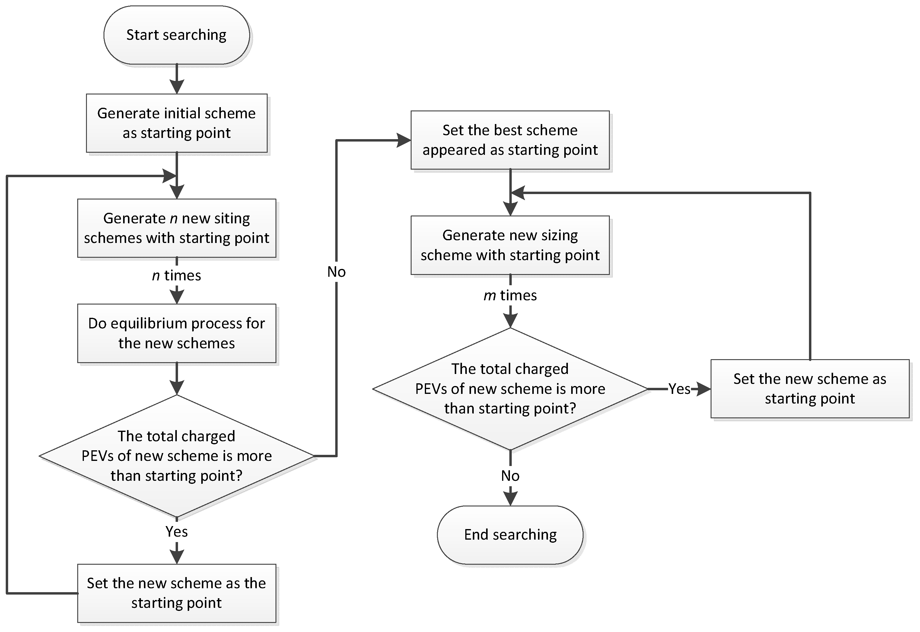
The flow chart of the entire algorithm is given in Figure 3.

3. Results

In this section, a case study from the practical highway network in Hunan is discussed to test the performance of the new local search algorithm and conduct managerial analysis. The endurance range of a BEV is assumed to be 150 km. The number of BEVs that can be charged by a charging pile per day is assumed to be 40. The constructing fee of a charging station is set to be 1.5 million, while the charging pile is 0.15 million. The total investment is set to be 750 million. All the currency discussed here is in USD. All the computational experiments are conducted on a Dell laptop with a 2.8 GHz Core-i7 processor and 16 GB RAM.

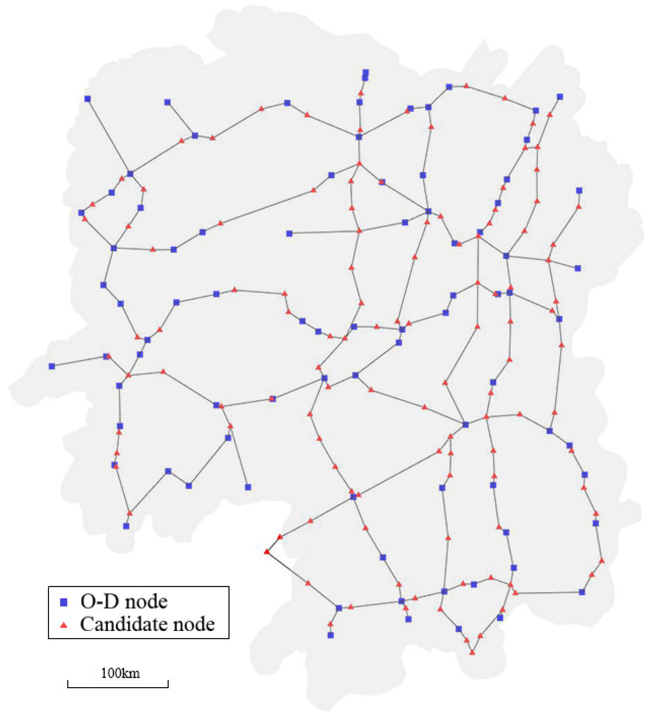
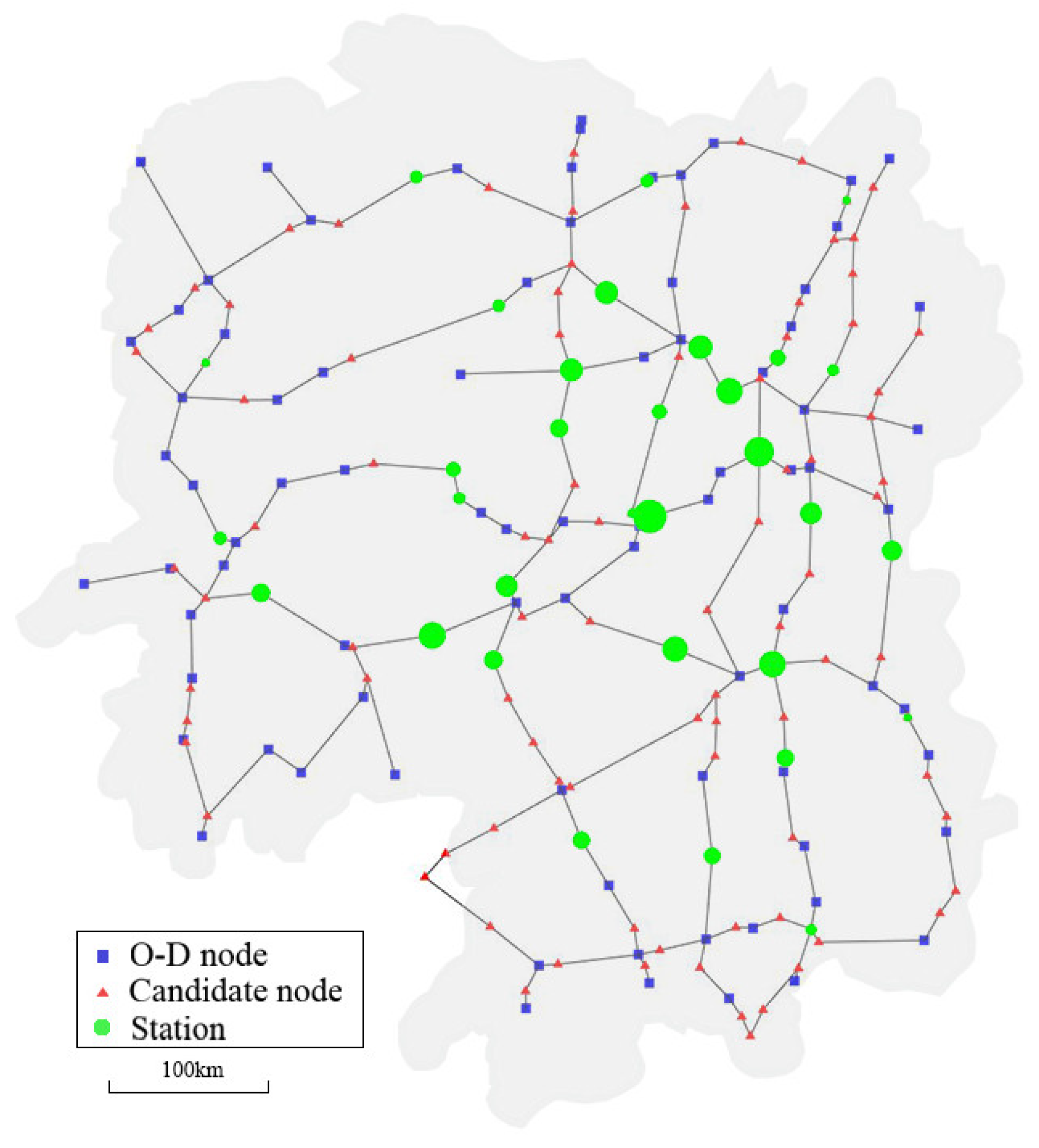
The Hunan highway network is shown in Figure 4, and comprises 85 O–D nodes denoted by blue rectangles, 118 candidate nodes denoted by red triangles and 225 arcs. The potential flows in the network are set in the same way as Hodgson [6], which is expressed by Equation (22):

$$f(i,j)=k{p}_i{p}_j/di{s}_{(i,j)}$$

(22)

where $f(i,j)$, $di{s}_{(i,j)}$ denote the potential BEV flow and the distance between node $i$ to $j$ respectively, $p_i$ denotes the population in node $i$, and $k$ is a coefficient.

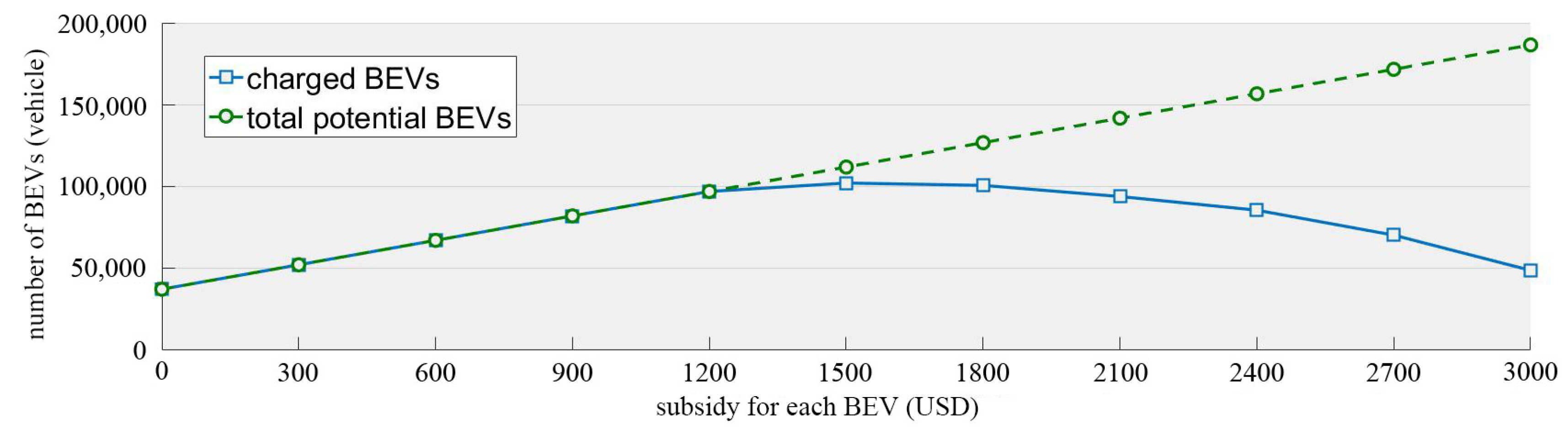
Figure 5 shows the optimizing results of LS under different subsidies. The results are the mean value of running this 20 times. When the subsidy for each BEV reaches 1500, the constructed infrastructure cannot fulfill all the potential demand. When the scale of the subsidy continues growing, there is even less budget for constructing infrastructure. Thus, the maximum amount of charged BEVs must appear in the situation that the constructed facilities can just fulfill the entire potential demand. However, the subsidy offered by the government cannot be accurate to detail this number, which is always a whole hundred number, and we only need to compare the results around the separating point like 1200 in Figure 5.

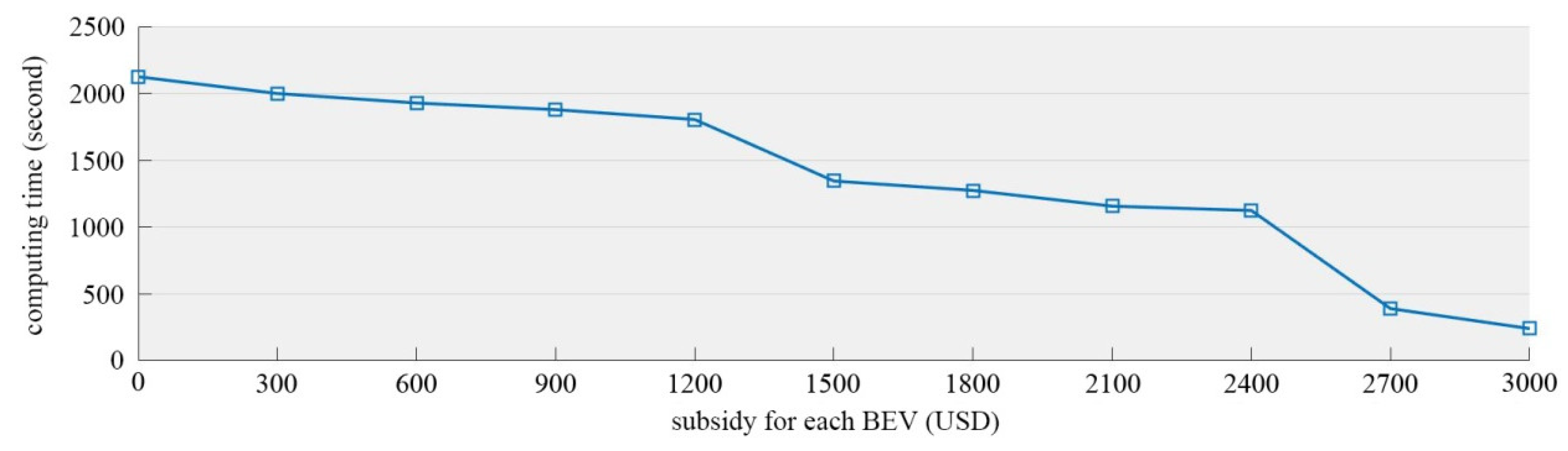
Figure 6 shows the computing times of the LS under different subsidies. The computing times are the mean value of 20 times running. The computing time stays in a high level when the subsidy is under 1200, because all the potential demand needs to be considered as the construction fee is sufficient. Then, the computing time begins to decrease when the subsidy is between 1200 to 2400. In this region, the potential demand cannot be fulfilled, but the convergence of LS is slow as there are many available siting and sizing schemes. When the subsidy reaches 2700, the computing decreases swiftly as the construction fee can only afford to build a few charging stations, which leads to the rapid convergence of the search. In general, the LS can obtain the solution with acceptable time cost.

The boxplot of running the local search 20 times is shown in Figure 7. To promote the stability of the LS, the y-axis presents the proportion of the difference between the results and the mean value. As we can see in Figure 6, when the subsidy is below 1500, the LS can always find the solution that meets all the potential demand. When the subsidy reaches 1500, the maximum difference does not exceed 4.0%, which proves a reliable stability of the LS.

The best scheme of siting and sizing is shown in Figure 8, in which the green circles denote the optimal location and size of charging stations. There are a total 32 stations and 3356 charging piles with the total construction fee of 551.4 million, while the total subsidy is 198.6 million. The stations are widely distributed in the network, of which the majority is concentrated in the north-east part of the network, as it is the most populous area of Hunan. There are only some small stations constructed in the north-west part of the network as it is a mountainous area with low population. The result reflects well the real situation of demand distribution. The result well follows the rules of utility theory, which gives the final choice of drivers that can achieve maximum probability of the charging service. In the situation of this result, no one is willing to change their scheme of charging, as have less opportunity to charge their vehicles.

Next, some managerial analyses are conducted to discuss some aspects that impact the budget arrangement and the siting and sizing strategy.

3.1. Impact of the Subsidy on the Siting and Sizing Strategy

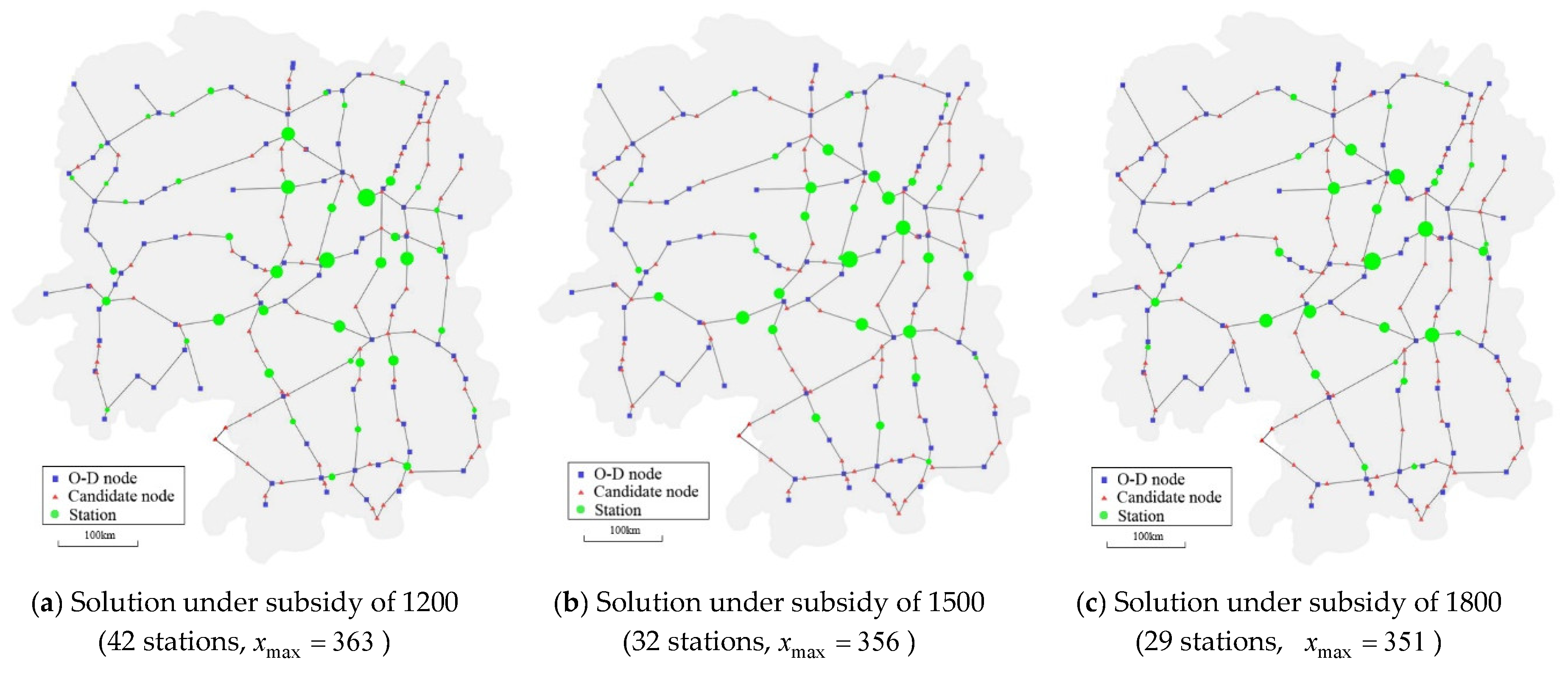
Figure 9a–c presents the deployment of the charging station with the subsidy from 1200 to 1800 for each BEV. When the subsidy is low, the charging stations spread all around the network to catch as much demand as possible. The proportion of the construction fee decreases when the subsidy rises, which leads to the reduction of the station quantity. As the potential BEV flow grows with the subsidy, the stations become more concentrated in the high distribution area of charging demand. Thus, a high subsidy may reduce the scope of the station deployment, which is not advantageous for promoting the adoption of BEV.

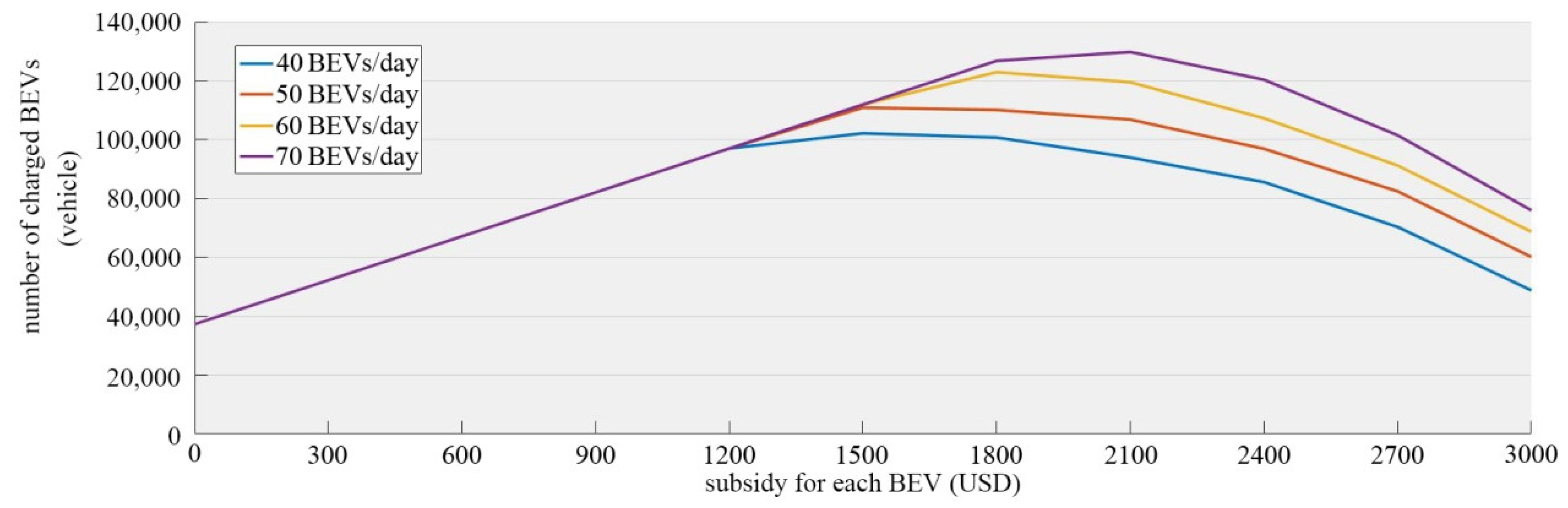
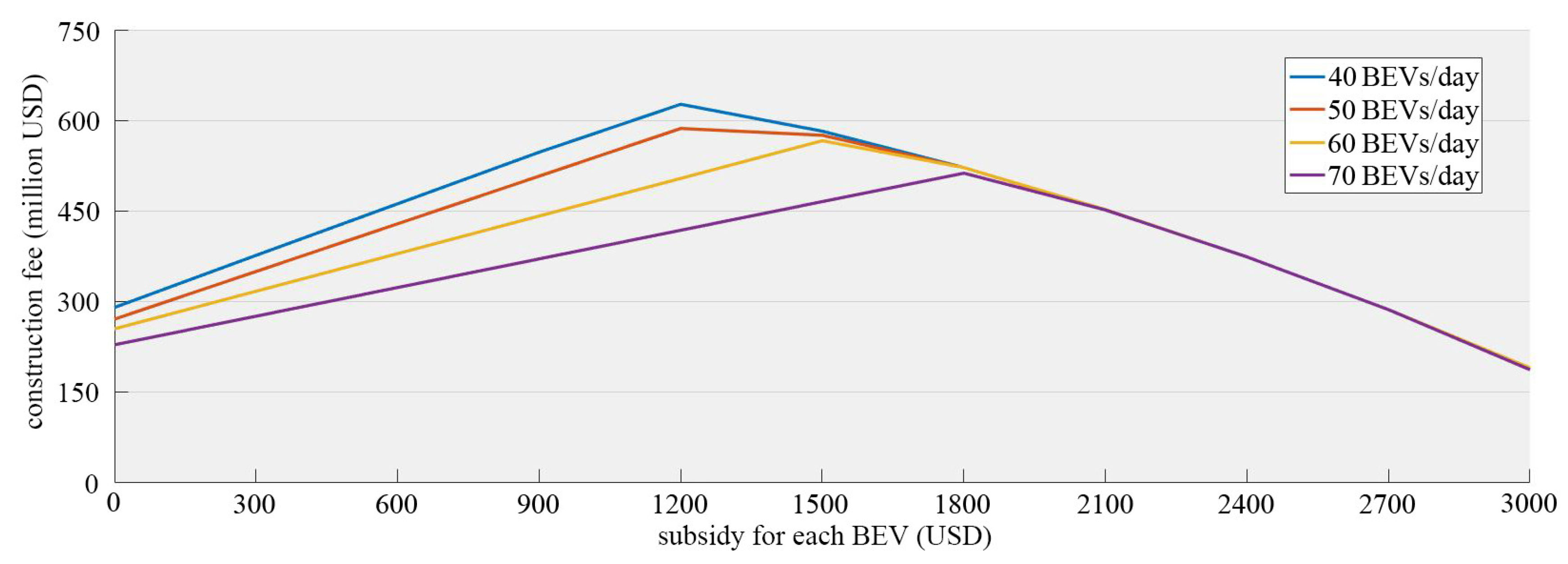
3.2. Impact of the Capacity on the Budget Arrangement and the Total Charged Flow

The results of the total traffic in the network and the budget arrangements are shown in Figure 10 and Figure 11, in which the capacity of the charging pile ranges from 40 to 70 and the endurance range is set to be 150 km.

Table 1. The best arrangements of the budget under each capacity.

Capacity (vehicle/day)	40	50	60	70
Construction (million)	582.15	575.40	521.85	451.80
Subsidy (million)	167.85	167.85	228.15	298.20
Available battery electric vehicles (BEV) (vehicle)	102,155	110,860	122,914	129,775

lists the total subsidy and construction fee of the best solution under each capacity.

As we can see from Figure 10 and Figure 11, when the subsidy is below 1500, the budget is sufficient to charge all the potential demand. The number of charged BEVs does not increase with improvement of the capacity. However, the construction fee decreases as the facilities have larger capacity that can charge more BEVs. When the subsidy is beyond 1500, the left budget cannot afford to charge all the potential demand. Thus, the left budget must be fully used to meet as much demand as possible. As the construction fee is fixed, the facilities with larger capacity can meet more potential demand. To illustrate the impact of the capacity on the subsidy, the best arrangements of the budget are listed in Table 1. We can find that the improvement of the capacity will lead to the proportion addition of the subsidy.

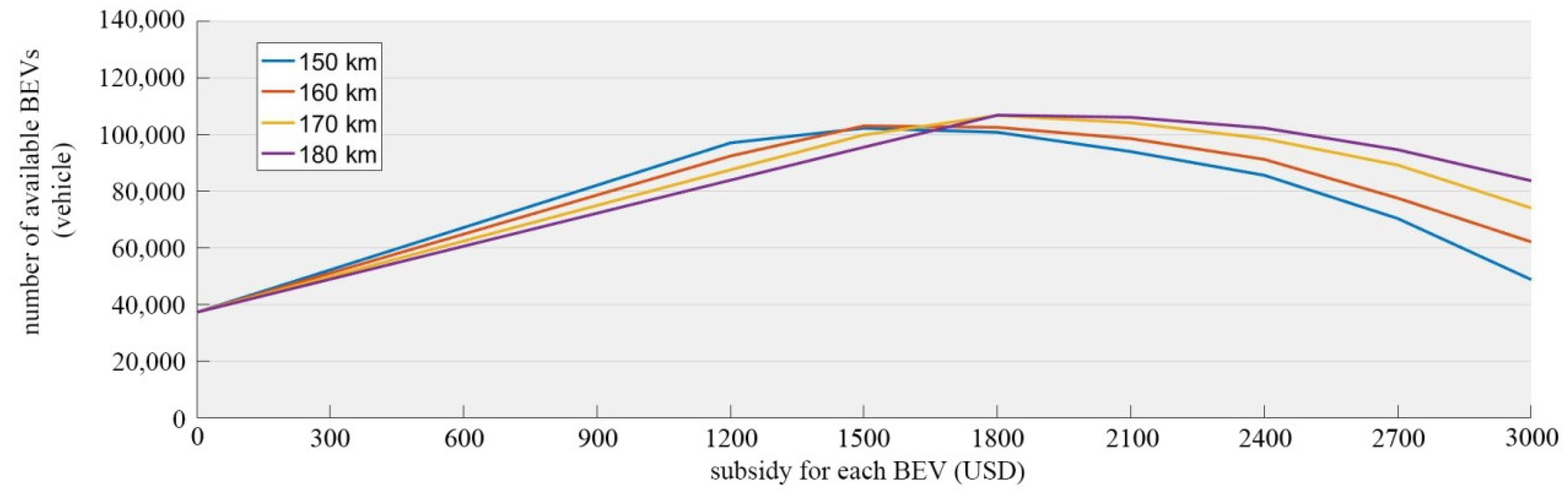
3.3. Impact of the Endurance Range on the Budget Arrangement and Total Charged Flow

When the endurance range rises, some BEVs do not need to recharge during the trip. Then we need to discuss whether this part of the demand should be subsidized. If we do not subsidize the recharge-free BEVs, the potential demand of this part will not increase with the subsidy. The optimization results under different subsidies would be like those in Figure 12 and Figure 13, in which the capacity of the charging pile is set to be 40 BEVs per day. To emphasize the different impact of the endurance range and the charging capacity, we add the recharge-free BEVs into the total charged BEVs, which is named “available BEV” in the y-axis.

When the endurance range rises, the potential demand decreases as the proportion of unsubsidized demand increases, which can be seen in the left part of Figure 12. There is more investment that can be used for facility construction, which can be seen in the right part of Figure 13. From

Table 2. The best arrangements of the budget under each endurance ranges.

Range (km)	150	160	170	180
Construction (million)	582.15	595.20	558.00	572.10
Subsidy (million)	167.85	154.80	192.00	177.90
Available BEV (vehicle)	102,155	102,975	106,631	107,125

, we can see that there is no large growth on the number of the total charged BEVs.

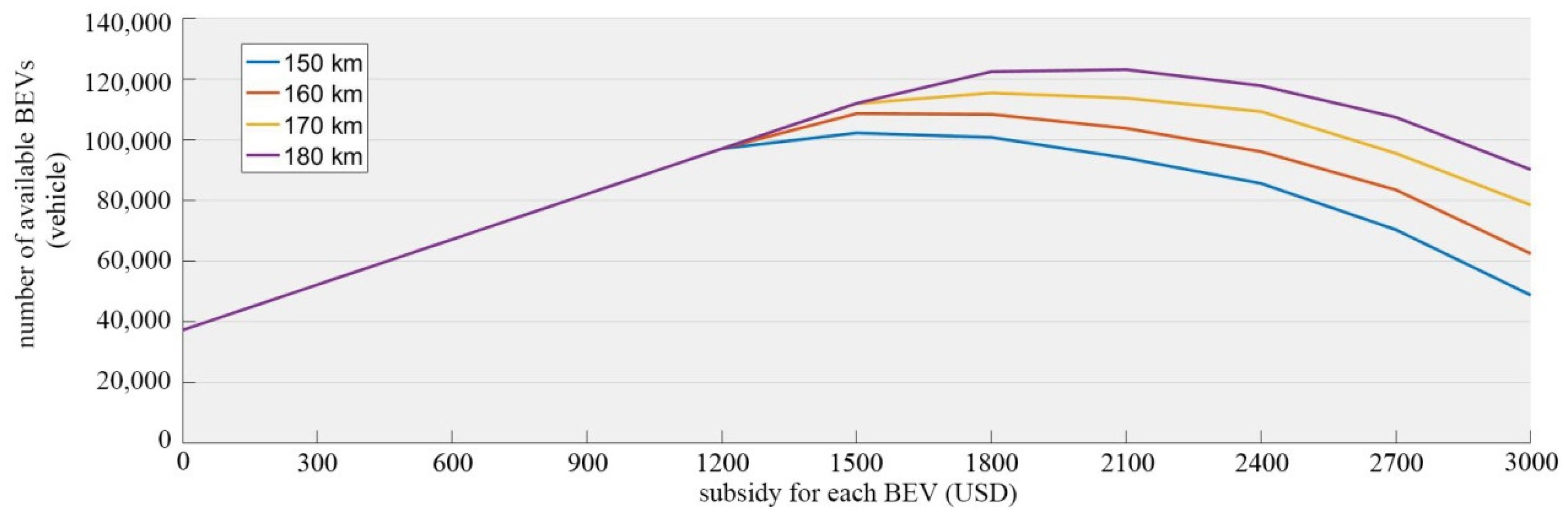
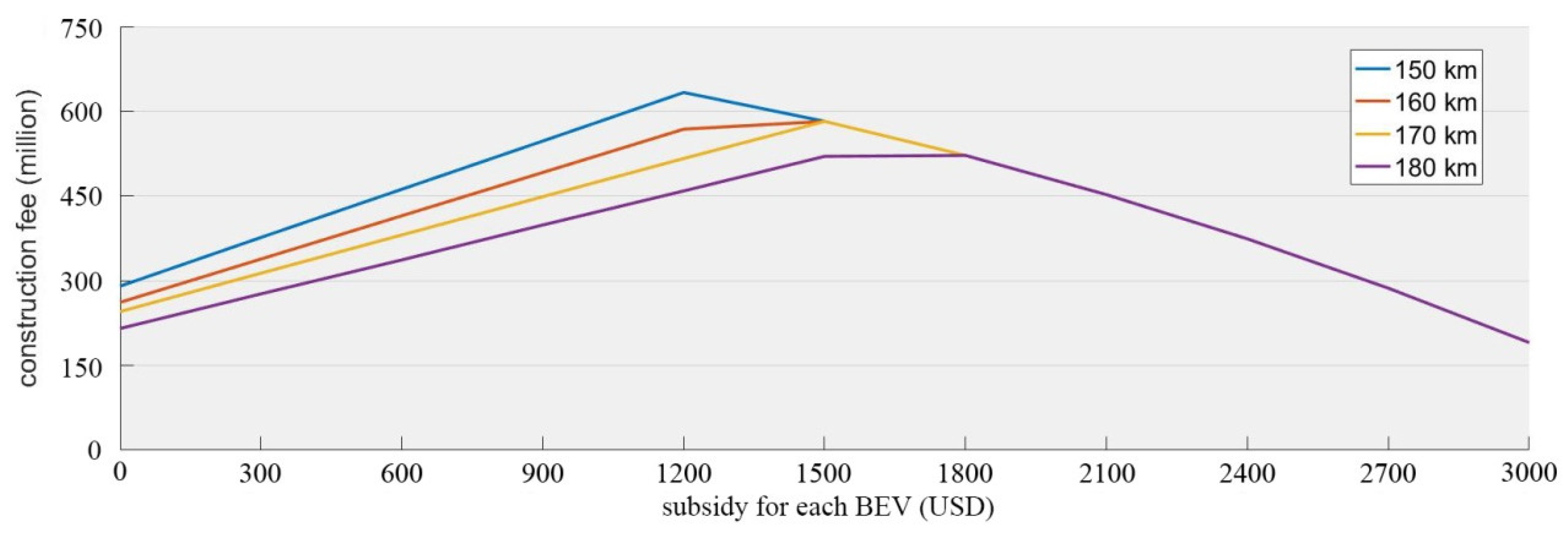
If we subsidize the recharge-free demand, the result should be like in Figure 14 and Figure 15. The growth trend in Figure 14 is much like that in Figure 10, and so is the construction fee in Figure 11 and Figure 15. From the best arrangement in

Table 3. The best arrangements of the budget under each endurance range.

Range (km)	150	160	170	180
Construction (million)	582.15	582.15	521.85	452.40
Subsidy (million)	167.85	167.85	228.15	297.60
Available BEV (vehicle)	102,155	108,546	113,330	123,006

, the improvement of the endurance range leads to the increasing proportion of subsidy. Thus, it is proved that more charged BEVs can be obtained when we subsidize the recharge-free BEVs.

Comparing the data in Table 1 and Table 3, we can achieve nearly the same number of the available BEVs in the network by raising 30 km of the endurance range or increasing 20 BEVs/day of the capacity. Despite the input–output rate of upgrading, the improvement of the endurance range is more efficient, of which 20% improvement can achieve the same effect as 50% improvement on the capacity. However, the proportion of the construction fee is larger when we choose to upgrade the capacity. If the budget and the achieved traffic are both the same, it is better to spend more money on construction which can be directly transformed into basic infrastructure. Thus, which aspect is more valuable depends on the practical requirement and the input–output rate.

4. Discussion

The optimization model and method in this paper is developed to help the government make policy on the budget arrangement and construction scheme. We provide an appropriate way to measure the impact of the subsidy by relating with the potential BEV flow, with which the optimization in the budget and construction can be discussed together. Meanwhile, the range restriction of BEV, the capacity restriction of charging stations, and the utility of drivers are all considered and formulated in the optimization model to make the solution more reliable. The result shows that the location and size of stations fits the population distribution well, which proves the usability of the model and method. Besides, the model and method allows the policy maker to compare different schemes by estimating the amount of BEV traffic.

The result shows that the largest number of charged BEV appears when the potential charging demand can just be fulfilled by the constructed facilities. Thus, the major issue of policy optimization is to find the “match point”. However, the relation between the subsidy and the potential BEV flow is not simply linear in some situations, which will cause multi-peaks in the curve of the subsidy and the number of charged BEVs. For this situation, we need to test more values of a subsidy to find out all the “match points”.

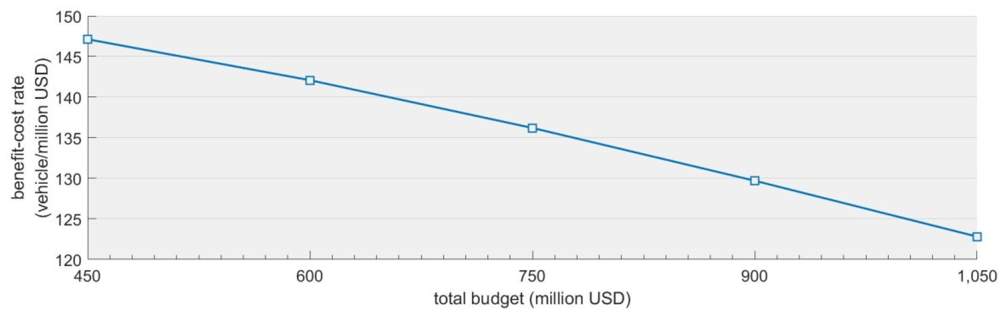
Another issue is the benefit–cost rate of the budget. We take the best solutions under the budget of 450, 600, 750, 900 and 1050 million dollars to draw the curve of the benefit-cost rate, which is shown in Figure 16, in which the unit of y-axis is added per vehicle per million dollars. The benefit–cost rate decrease linearly with the budget. This is because when the total budget rises, the “separate point” moves right. The total subsidy increases with a quadratic growth while the budget increase linearly. The proportion of the construction fee continues decreasing in the best solution, which explains the reduction of the benefit–cost rate. However, in some situations, the major objective of the government is to increase the BEV traffic as much as possible. In spite of the low benefit–cost rate, the policy maker will also place a large amount of the budget in adopting BEVs.

Although we take the major restrictions into consideration, there are still some issues that need to be further discussed. The ranges of BEVs are set to be a fixed value, and this value may vary with the vehicle model, terrain, temperature, traffic intensity and other factors, which needs to be refined and classified. Besides, the advertising effect needs to be considered in expanding potential BEV flow.

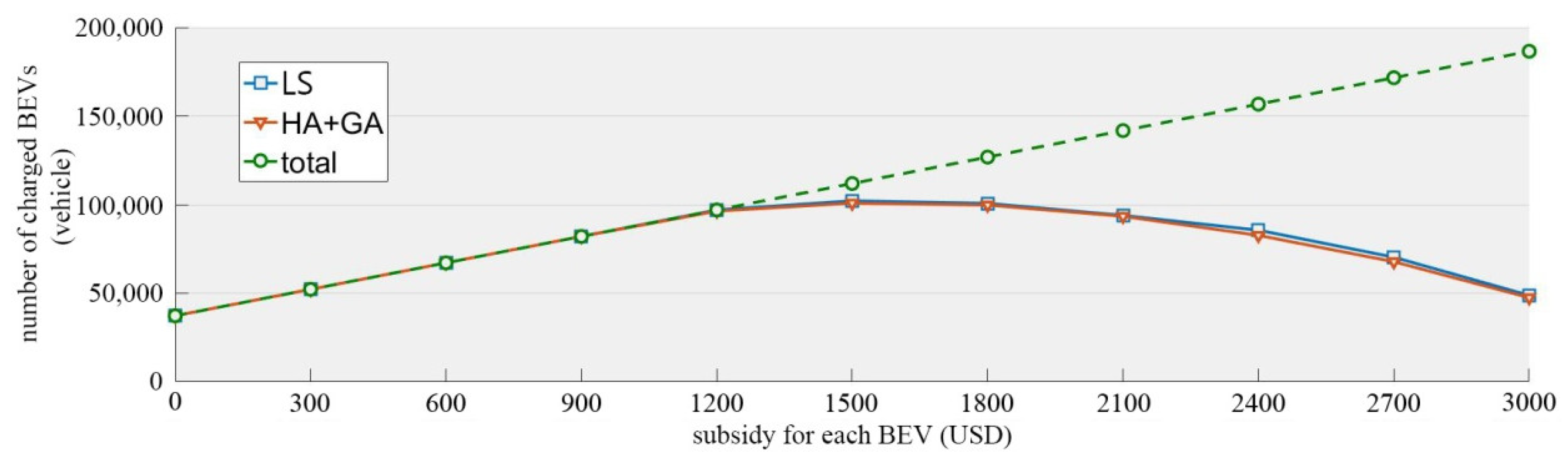
To maximize the charged BEV numbers, a sizing optimization is added into the local search algorithm. The result only proves the usability of LS, whether the solution is sufficiently optimal is not identified. To test the efficiency and effectiveness of LS, we compare it with the genetic algorithm with initial population generated by a heuristic algorithm (HA + GA) in the Hunan highway network.

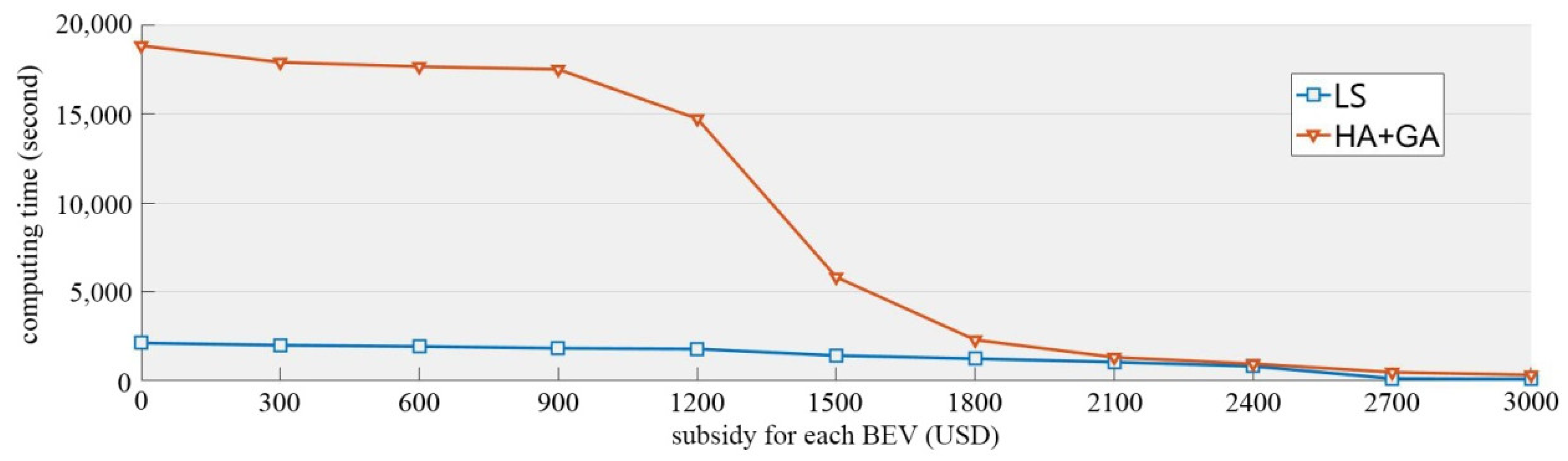
Figure 17 and Figure 18 show the results and the computing times of two algorithms under different scales of subsidy, respectively. The results and computing times are the mean values of 20 times running. From these figures, we can find that LS can achieve better solutions with less time than HA + GA. When the subsidy is equal to 1500, the volume of charged BEV flow reaches the largest value. The computing times of HA + GA are much longer than the LS when the subsidy is less than 1500. This is because when the subsidy is under 1500, the remaining budget is sufficient to fulfill all the potential demand in the network, which means the $f_{qh}$ of all combinations for all paths are computed. The schemes generated by HA + GA always cover the potential demand completely as all the stations are recorded in the chromosome. Once there is budget left, the new stations are added into the scheme continuously. However, there may be some schemes generated by LS that only cover part of the potential demand, which avoids much computing complexity.

To further test the efficiency and effectiveness of the LS, we exploit the artificial network of different scales in [15]. The results and computing times of two algorithms are shown in

Table 4. Computational results of the three algorithms for the artificial networks with different scales.

Algorithms →	Heuristic Algorithm (HA) + Genetic Algorithm (GA)		Local Search (LS)		HA + GA + LS
Network Size (N1/N2/N3) ↓	Volume	Time	Volume	Time	Volume	Time Addition
50/90/151	65,119.73	113.23	65,315.29	177.55	65,752.38	134.93
50/93/156	38,294.41	790.03	38,295.01	576.97	38,419.57	67.49
50/95/154	45,767.77	770.18	46,394.62	124.74	47,070.83	102.86
50/99/157	46,782.00	438.98	46,835.82	310.04	46,886.07	150.57
50/99/162	50,700.75	503.20	50,851.82	473.35	50,889.77	318.19
50/101/162	34,570.00	895.61	34,285.30	333.02	34,570.00	39.51
50/102/164	37,604.62	555.87	37,758.62	374.65	37,783.51	156.64
50/107/174	37,583.09	361.33	36,934.05	197.67	37,603.81	103.87
50/111/173	47,875.24	247.47	47,045.83	63.01	47,987.81	50.17
50/114/184	52,005.95	164.23	52,125.62	254.78	52,236.90	152.77
100/204/261	78,679.07	682.63	79,297.74	892.58	79,440.19	473.40
100/204/334	99,033.50	545.12	100,635.72	511.91	100,741.43	500.27
100/214/346	62,956.73	1775.16	61,485.80	813.67	63,519.85	851.66
100/214/352	77,542.67	741.80	77,826.31	712.67	77,893.22	442.11
100/222/356	80,085.25	682.36	80,420.98	500.35	81,201.74	262.28
100/222/360	85,885.76	514.27	85,008.59	1507.46	86,488.73	673.09
100/224/376	112,074.84	685.13	105,854.52	314.41	113,418.98	797.54
100/224/358	91,362.32	436.12	91,503.94	233.12	92,483.70	137.82
100/227/359	71,555.30	1093.64	71,139.27	895.35	71,742.85	784.83
100/231/368	90,373.41	360.17	89,290.97	473.64	90,838.82	185.88

, which are the mean value of 20 times running. The unit of the volume is vehicle while that of the time is second. The results show that LS can obtain better solutions with less time cost in most cases. However, there are still some situations that HA + GA performs better. This is because that the quality of the LS solution relies much on the starting scheme, which limits the searching scope. However, if we define some jump-out procedures, the computing time is hard to control.

As the LS can improve the given solution, we treat the best solution of HA + GA as the starting scheme and resolve the artificial networks. The results are shown on the right of Table 4. We can find that LS can efficiently improve the solution of HA + GA with relatively shorter time cost. The solutions of HA + GA + LS are better than those of LS and HA + GA. Using the solution of HA + GA as the starting scheme can decrease the searching time in majority situation, because the solution of HA + GA is already optimal which means the number of jumps is fewer than before.

Furthermore, as the genetic algorithm can also improve the initial population. Then we add the solution of the HA + GA + LA as part of the initial population of GA and redo the optimization of the artificial networks, whose results are improved by the LS again. The results of the repeated optimization are shown in

Table 5. Computational results of the multi-optimization for the artificial networks with different scales.

Algorithms → Network Size (N1/N2/N3) ↓	HA + GA + LS	GA + LS 2	GA + LS 3	GA + LS 4	GA	LS
50/90/151	65,752.38	66,037.80	66,047.80	66,047.80	65,582.12	65,638.89
50/93/156	38,419.57	38,428.08	38,884.01	38,884.01	38,765.18	38,333.89
50/95/154	47,070.83	47,070.83	47,070.83	47,070.83	46,353.49	46,580.49
50/99/157	46,886.07	47,218.00	47,554.54	47,554.54	46,960.08	46,922.93
50/99/162	50,889.77	51,010.00	51,010.00	51,010.00	51,003.43	50,950.13
50/101/162	34,570.00	34,570.00	34,570.00	34,570.00	34,570.00	34,434.76
50/102/164	37,783.51	37,801.29	37,816.32	37,816.32	37,778.87	37,781.62
50/107/174	37,603.81	37,653.82	37,677.00	37,677.00	37,645.61	37,016.21
50/111/173	47,987.81	48,032.21	48,194.07	48,194.07	47,924.20	47,641.68
50/114/184	52,236.90	52,254.42	52,436.70	52,436.70	52,283.04	52,193.86
100/204/261	79,440.19	79,503.53	79,558.85	79,558.85	79,370.52	79,420.70
100/204/334	100,741.43	100,741.43	100,741.43	100,741.43	99,363.11	100,707.59
100/214/346	63,519.85	63,639.26	63,866.67	63,866.67	63,589.32	63,456.07
100/214/352	77,893.22	78,333.49	78,459.04	78,459.04	78,198.91	77,858.10
100/222/356	81,201.74	81,253.62	81,921.20	81,921.20	81,077.45	80,647.70
100/222/360	86,488.73	86,828.85	87,069.35	87,069.35	86,447.95	86,290.00
100/224/376	113,418.98	114,302.41	115,196.83	115,196.83	113,557.71	108,398.17
100/224/358	92,483.70	92,534.67	92,534.67	92,534.67	91,832.82	91,921.80
100/227/359	71,742.85	71,972.00	72,015.51	72,015.51	71,588.38	71,526.71
100/231/368	90,838.82	91,686.27	93,172.09	93,172.09	91,310.04	90,380.06

. We find that the multiple running of GA + LS can further improve the solution. The improvement finally reaches stability since the fourth running. The two columns on the right are the results obtained by GA and LA with the same time cost of GA + LS 4, which proves that the repeat use of GA + LS can effectively improve the quality of the solution.

5. Conclusions

This study investigates the joint policy optimization problem for a subsidy on electric vehicles and infrastructure construction in the highway network. The optimization model and method is proved to be useful for helping policy makers achieve a maximum number of charged BEVs with a given budget. The local search is able to improve the solution obtained by other algorithms, of which multiple running will bring even better solutions.