Economic Optimal Implementation of Virtual Power Plants in the German Power Market

Candra, Dodiek Ika; Hartmann, Kilian; Nelles, Michael

doi:10.3390/en11092365

Open AccessArticle

Economic Optimal Implementation of Virtual Power Plants in the German Power Market

by

Dodiek Ika Candra

^1,*,

Kilian Hartmann

^2,* and

Michael Nelles

^1,3

¹

Department of Waste & Resource Management, Faculty of Agricultural and Environmental Science, University of Rostock, 18059 Rostock, Germany

²

Department of Engineering Science, Faculty of Engineering, Aschaffenburg University of Applied Sciences, 63743 Aschaffenburg, Germany

³

Deutsches Biomasseforschunsgzentrum gGmbH (DBFZ), the Centre for Biomass Research in Germany, 04347 Leipzig, Germany

^*

Authors to whom correspondence should be addressed.

Energies 2018, 11(9), 2365; https://doi.org/10.3390/en11092365

Submission received: 9 August 2018 / Revised: 22 August 2018 / Accepted: 5 September 2018 / Published: 7 September 2018

Download

Browse Figures

Versions Notes

Abstract

:

The burden of excess energy from the high renewable energy sources (RES) share creates a significant reduction of residual load for the future, resulting in reduced market prices. The higher the share of stochastic RES, the more often the price will be 0 €/MWh. The power market needs new methods to solve these problems. The development of virtual power plants (VPPs) is aimed at solving techno-economic problems with an increasing share of RES in the power market. This study analyses a possible implementation of stochastic and deterministic RES in a VPP to generate secured power, which can be implemented in the European Power Exchange (EPEX)/European Energy Exchange (EEX) power market using existing market products. In this study, the optimal economic VPP configuration for an RES-based power plant is investigated and implemented into standard power market products. The results show that the optimal economic VPP configuration for different market products varies, depending on the energy availability and the marginal costs of the VPP components. The size of the VPP components is positively correlated to the components’ share of the energy generated. It was also found that projecting or implementing VPPs in Germany at current market prices (EPEX/EEX prices) is not yet economically feasible for a small share of market products. However, the secured power can be marketed on the SPOT and in the futures market with higher and more stable prices compared with the status quo.

Keywords:

VPP; marketing; configuration; energy transition; power market; EPEX; EEX; power market products

1. Introduction

One of Germany’s energy transition plans involves increasing the share of renewable energy sources (RES) in total electricity consumption, in order to reduce fossil-fuel dependencies over a long term perspective. The RES share of gross electricity consumption in Germany in 2016 has reached about 31.7%, from a targeted share of 35% in 2020, and 80% in 2050 [1,2]. In 2015, Germany had a total power generation of 651.8 TWh (51.8 TWh were exported, and 30% originated from RES [3]). Until the end of 2014, the RES share was dominated by wind (77.3%), followed by solar photovoltaics (PV) energy (15.5%) and others (7.2%) [4]. The contributors of this high share of RES to the total amount of electricity generated are not only large-scale power generators, but also the owners of decentralized energy resources (DER) and small-scale RES-based power plants, such as solar PV from private owners [5].

The problem with this high share of stochastic RES in the total amount of electricity generated, and its simultaneous power generation, is the temporary surplus of power. This surplus leads to a drop of prices tending to 0 €/MWh in a free market [6]. The higher the share of stochastic RES, the more often the price will be 0 €/MWh. The power market needs new methods to solve these problems [7].

The development of virtual power plants (VPPs) aims to solve techno-economic problems regarding an increasing share of RES in the power market. The implementation of VPPs in the power market is a possibility to convert energy from stochastic power plants into secured energy by mixing it with small amounts of energy from deterministic power sources. This approach not only provides secured power [8,9,10,11,12,13,14,15,16,17], but also brings DER, including RES, to the power market, to become competitive, as compared with fossil-based energy generators [18,19]. The VPP is a part of the internet of energy (a scenario in energy transition) [20], and it is a mature technology that has already been implemented [21]. It has been shown that DER in a VPP gain more revenues than independent and non-market-oriented DER operations [22]. In the VPP, DER also have the flexibility to participate in many trading options in the power market, such as in the Day-Ahead and in the Intraday markets [23,24,25]. The studies from the literature [9,26] show that implementing RES in a VPP could reduce RES costs in short-term power markets, thus increasing benefits of RES.

Previous studies such as the works of [27,28] have explored the implementation of a VPP in the power market with different control schemes. Many of the studies also concern the stochastic and deterministic analysis for demand response, such as that by the authors of [29], which can help the VPP to cope uncertainties of RES. However, studies on optimal economic VPP configurations for RES-based power plants in the existing market products, especially in Germany’s power market, are still missing.

This study analyses a possible implementation of stochastic and deterministic RES in a VPP to generate secured power, which can be implemented to the EEX/EPEX power market using existing market products. In this study, the optimal economic VPP configuration for an RES-based power plant is investigated and implemented into standard power market products. The investigation on the projection of the VPP with different market products presents the idea to provide secured market products from the high RES share.

To address the issue in this study, the following steps are conducted:

Data collection of load schemes and market prices (EEX, EPEX) for several market products (base, peak, off-peak, etc.).
Adaptation of load data to the market products.
Design of adapted VPP configurations, including an optimization concept and an information communication technology (ICT) concept.
Balance of generation and load in an energy management algorithm.
Sensitivity analyses to adapt and test the VPP components on different market products.
Calculation of the contribution margin of the VPP in the analyzed scenarios.

This paper is organized as follows: In Section 2, materials and methods of the study are presented. In the materials part, the load profile, market prices, market products and adapted load profile to the market products are described. In the methods part, the configuration of the VPP, energy management, sensitivity analysis, and calculation of the contribution margin of the economic results are described. In Section 3, the economic optimal VPP configuration at different market products and contribution margin of the analyzed scenario results are presented. In Section 4, the results are analyzed, followed by the conclusions drawn in Section 5.

2. Materials and Methods

The VPP is yet to be defined, but has widely-accepted general concepts. With regards to previous studies [19,30,31,32,33,34,35,36,37,38,39], VPPs can be categorized into two main concepts: technical or commercial VPP. Technical VPPs (TVPPs) focus on technical operations and on the services of DER, whereas commercial VPPs (CVPPs) focus on TVPPs in markets operations. The technical operation functions include real-time and scheduled operations, aggregations, ancillary services, forecasting functions, and DER maintenance and submissions. Both TVPPs and CVPPs have the same VPP components, which consist of generation technology, energy storage, and information and communication technology (ICT). Moreover, the targets of VPPs, with controls as well as boundaries and forecasting functions, are added as a component of the VPP [18,33,40]. The targets of VPPs in this study can be explained as being market products from the VPP.

In this study, the VPP was built from the combination of a solar PV system, a battery system, and an adapted biogas power plant. The biogas power plant used in this research is adapted from the “Controlling of Gas Production in Biogas Plants (ReBi)” concept [41] as a flexible power generator based on demand-driven biogas operation principle. According to the literature [42], the VPP delivers secured power for different load demands. The VPP components are divided in two main systems, which are the hardware and intelligent systems (Figure 1). In the hardware system, all of the hardware components of the VPP were made up. These include an applications server, a database server, a web server, local controllers, a battery system, and a biogas power plant. The solar PV power plant is not depicted in Figure 1; because in this case, the generated energy from the PV was derived from the local operator as external data. In the intelligent system, the “brain” of the VPP is built. This includes optimization tools and visualization tools within a graphical user interface (GUI).

2.1. Material

2.1.1. Load Profile

A load profile is an important component for estimating the power markets [43], and it gives information about the load fluctuations or the load durations in the power markets over a specific period of time. In this study, there were no specific parameters to be considered when selecting which load data would be used as the load profiles in the VPP. It was assumed that the VPP needed to be capable of addressing several kinds of load conditions. The load profiles that had the maximum load data for winter and for summer were then selected, and these were used as load profiles in the VPP. Later on, if the VPP was to be applied to other load data, the VPP’s operator would be able to replace these load profile samples. The load data used in this study was derived from a local grid operator. There was a middle-size power plant in this grid, which influenced the expected standard load profile.

The following steps were conducted to generate a load profile from the load data for the VPP:

Visualizing the load data from a twelve-month load profile. The twelve-month load profile showed the load fluctuations over a year by representing a monthly range of load data. The twelve-month load profile of analyzed data (Figure 2) showed an overview of load conditions over the year 2015, which fluctuated between 8 MW and 110 MW.
Selecting a month. The maximum load range occurred during the winter and the summer periods. The load in January and the load in July from (Figure 2) were selected to represent the months that had the highest load levels in winter and summer, respectively. The four-week load data for these selected months were then visualized in an hourly-interval load profile (Figure 3).
Selecting a week load data from the selected months. There were no specific criteria in this study for selecting the weekly load data from the selected months over summer and winter (Figure 3). The second week in July and the fourth week in January were randomly selected to be analyzed in this study (Figure 4). These weekly load data over summer and winter were then used in the Week Futures (WF) market.
Selecting two days from the weekly load profiles over summer and over winter as the samples of the load profiles in the Day-Ahead (DA) market in the SPOT market. As can be seen in the load profile in Figure 4, the highest loads during workdays in winter or in summer occurred on Monday, whereas the highest loads during weekends in winter or in summer occurred on Saturday. Thus, Monday and Saturday were selected to be used in the Day-Ahead market operation of the VPP (Figure 5).

2.1.2. Market Prices Data and Market Products

The market products of the VPP totaled 9 × 68 products for the Day-Ahead market, and 9 × 4 products for the Week Futures market (Appendix A, Table A1). In the Day-Ahead market, there were 17 types of market products (Table A2), based on the time for when the load was required, such as the peak load bid for a load between 08:00 and 20:00 [44]. In the Week Futures market, the market’s products were the base load and peak load in summer or in winter. Nine (9) was a factor that represented the nine VPP configurations.

The market prices in the Day-Ahead or in the Week Futures market were constant over a specific time, for instance, the prices for peak load were constant from 08:00 to 20:00 [45]. Peak load demand occurred from Monday to Friday. A sample of the market prices for peak load in the Week Futures market can be seen in Figure 6. The complete market prices for both market types are provided by Table A3.

2.1.3. Adaptation of Load Data to Market Products

The load profiles from Figure 4 and Figure 5 needed to be adapted to the market products. In this case, the volumes of the load demands in the Day-Ahead and the Week Futures markets were made constant for a specific period of time, referring to the literature [44]. For instance, the base load had a constant load over a 24 h period. The market prices and bid volumes of each of the market products were generated by a market mechanism where the demand and supply met. Equations (1) to (8) were considered based on the literature [46].

The bid volumes of the specific market products x in this study were then determined by Equation (1):

{BVOL}_{x} = \sum_{k = 1}^{n} c_{x, k} . (\frac{\sum_{k = 1}^{n} (g_{x, k} . {Pres}_{l, k})}{s_{x}})

(1)

The base load calculation was made as in Equation (2):

{Pbase}_{l, k} = {Pavg}_{l, k} - {Paravg}_{l, k}

(2)

If a total load of the market category l was subtracted by the base load of the market category l, then there would be remaining load demands that were part of the total load, but not the part of the base load. In order to know whether there were any remaining load demands, Equation (3) was conducted:

{Pres}_{l, k} = {Ptot}_{l, k} - {Pbase}_{l, k}

(3)

This remaining load signal was then calculated using Equations (4) and (5):

g_{x, k} = 1 ({when Pres}_{l, k} > 0)

(4)

g_{x, k} = 0 ({when Pres}_{l, k} < 0)

(5)

The number of remaining load demands’ signals for the market product x were then calculated by Equation (6):

s_{x} = \sum_{k = 1}^{n} g_{x, k}

(6)

In order to simplify the process calculation and to reduce the processing time in the VPP in the Week Futures markets, Equation (7) for winter and Equation (8) for summer were then used to calculate the peak load in the Week Futures markets:

{Ppeakw}_{w} = 2. . {Paravg}_{5, k}

(7)

{Ppeakw}_{su} = 2. . {Paravg}_{6, k}

(8)

The samples of these bid calculations for the Day-Ahead and Week Futures markets are depicted in Figure 7a–d and Figure 8a,b. The other bid type volumes are not depicted in the figures, but they are explained in Table A4.

2.2. Methods

2.2.1. The Configuration of the VPP

The VPP was configured using two main methods: the optimization algorithm and the method for the ICT configuration of the VPP. The optimization concept was built as in the literature [42] to optimize the utilization of every single component in the VPP, such as a local controller in the biogas power plant. In the end, there would be a collection of entities in the VPP, which would collaborate with each other to meet common targets, that is, to address load demands. Energy and information exchanges are conducted by these entities in the exchange lines during the operation of the VPP (Figure 9).

The ICT components of the VPP were built as in the literature [47], based on the openness of the VPP components for future ICT developments. The ICT components of the VPP included the use of state-of-the-art advanced ICT security technology (virtual private network (VPN)), cloud computing, and exchange protocols (open platform communications (OPC), transmission control protocol-internet protocol (TCP-IP)). The main backbone of the ICT concepts for the VPP was the intensive use of open-source software based on community-based developments.

2.2.2. Energy Management

The energy management of the VPP was based on an energy management plan as given in the literature [42], and an added component at the end of the energy exchange phase. The added component was a comparator that was intended to minimize the gap between the planned and the measured exchanged energies in the VPP. The merit order calculation was used as a strategy to aggregate the energy from the integrated energy sources (IES) [48]. The complete calculation of the IES cost and optimization was previously calculated in the literature [42]. To maintain security for the supply, with reduced generation costs in the VPP, the following considerations were taken into account for this VPP (Figure 10), as given in the literature [42]:

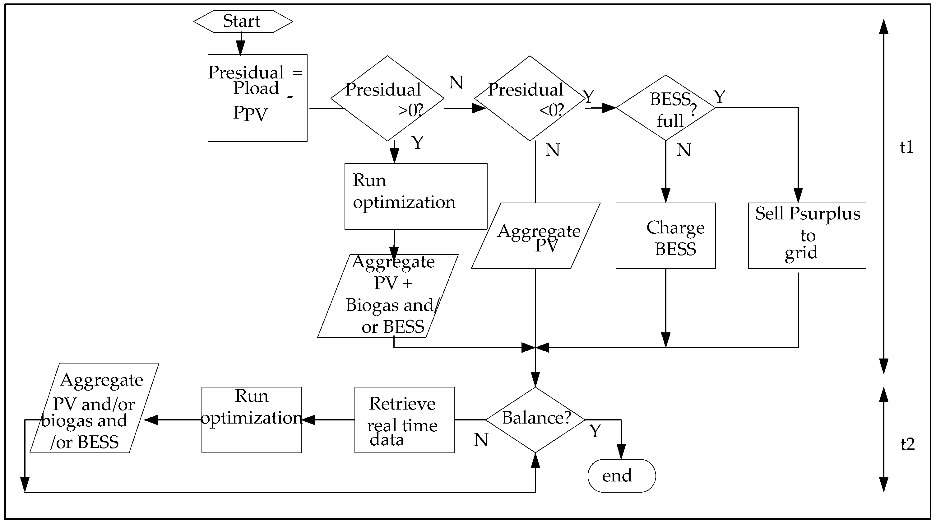
(a): The highest priority to meet the load demand was given to the power plants with the lowest marginal costs. Assuming that the sorted power plants, as based on marginal costs from the lowest to the highest, were the solar PV, the battery energy storage system (BESS), and the flexible biogas, the solar PV thus had the highest priority to meet the load. If the solar PV did not generate enough energy to meet the load, then the energy from the flexible biogas would be combined with the energy from the BESS (if applicable). If the solar PV generated more energy than the load, then the surplus energy from the solar PV would be stored into the BESS (in the case that state-of-charge (SOC) <100%, otherwise there would be nothing to do).
(b): As a result of biological constraints such as digestion time, the flexible biogas may need more time to aggregate its energy than the BESS. Thus, a BESS is still needed to support the flexible biogas in the operation of the VPP. If more/different intermittent RES were installed, that is, wind turbine power plants, the contribution of the BESS in the load could be minimized.
(c): The energy exchange was calculated at time t1, and then it was optimized again at time t2. Time t1 is the time when the aggregator or the operator makes the dispatch schedule for the Day-Ahead or Week Futures markets, such as on the day before the required delivery time for the energy. Time t2 is the minimum time required to compensate the gap between the scheduled and the measured exchanged energies. The balance of generation and load in an energy management system at time t2 is conducted by a comparator algorithm. Future investigation of time t2 should be conducted in practical implementation. In this study, t2 was determined to be about 2 ms with reference to the measured exchange rate in the literature [47].

In contrast to previous studies [49,50,51,52], the priority of the VPP implementation in this study was to provide secure power supply. It was assumed that all of the power plants of the VPP were participants in the energy market. However, the mechanism for selling surplus energy to the grid in this study was not economically considered, but it was instead considered as an energy surplus.

2.2.3. Sensitivity Analyses

A sensitivity analysis was conducted by adoption and testing of the VPP components from different market products. The previous composition of the solar PV, the BESS, and the flexible biogas (Table 1, refer to Table 2 configuration 1) was scaled up and it was compared with other compositions such that at the end, there were nine configurations that were used for sensitivity analyses (Table 2). It was assumed that marginal costs of PV were 0 €/kWh, the BESS marginal cost varied (depending on market prices associated with the scenario +10% losses), and the biogas marginal cost was 15 cents €/kWh based on calculation derived from previous studies [53,54,55,56,57,58]. The optimal economic VPP configuration for different market products was analyzed by evaluating the optimal economic contributions of the VPP components, based on these nine VPP configurations.

2.2.4. Calculation of the Contribution Margin of the Economic Results

To calculate the profits or losses of the economic results from energy management of the VPP, the cost analysis was performed by adopting the method conducted by the authors of [59]. The marginal costs and the market prices were compared in order to reveal the contribution margin of the VPP. The analysis based on marginal cost was aligned with one of the core features that was proposed by EPEX SPOT and EEX in further developments of the “erneubare energien gesetz” (EEG) [60]. The contribution margins were then calculated based on Equation (9) to 9 VPP configurations (Table 2):

{CM}_{l} = {MP}_{l} - {Copt}_{l}

(9)

3. Results

When the 9 configurations of a total of 68 VPP products for the Day-Ahead market, and 4 products for the Week Futures market, were applied to energy management systems and Equation (9), the economic optimal VPP configuration and contribution margin of the different load schemes were quite different.

As an observation of VPP implementation in different load schemes, it was apparent that the share of the VPP’s components in an optimal economic VPP configuration varied over weekday/weekend times, seasonal times, VPP component sizes, and the type of markets presented (Figure 11). As expected, the sizes of the VPP components had an influence on the share of power generated by the VPP components in economic and optimal VPP configurations. In the analyzed load schemes, VPP size enlargement had a positive correlation with the share of electricity from the VPP components that had minimum marginal costs. On the weekend, compared with the weekdays, the VPP required more energy from biogas. In the Week Futures market, the share of PV was not as high as it was in the Day-Ahead markets.

In the Day-Ahead market in winter, the VPP used more than 72% of its total energy from biogas in Configuration 1 (Figure 11a). When the sizes of PV and BESS were increased, the share of biogas in the VPP could be reduced to 53% in Configuration 9 on Monday. The increasing size of PV from Configuration 1 to 9 allowed the PV to increase its share in the energy generation of the VPP up to 41.5% on Monday in Configuration 9. The BESS has the smallest contribution to the total energy used in the VPP, with a maximum of 8% share on Monday in Configuration 3. Increasing the BESS size by Factor 3 caused an increase in the BESS share in the VPP’s energy output of almost three-fold.

In the Day-Ahead market in summer, 60% of the total energy of the VPP was generated by PV. The maximum PV share in the VPP was about 80% in Configurations 7, 8, and 9 on Monday (Figure 11b). The rest of the share of the VPP was generated by biogas and BESS. The maximum biogas share in the VPP was a quarter of the total in Configuration 1 on Monday. This share decreased when the sizes of PV and BESS were increased. The use of BESS in the Day-Ahead market and in the Week Futures market in winter was relatively low (up to 10% in Configuration 3). Increasing the BESS size by a factor of 3 caused the BESS to take up an increased share of the VPP’s power generation by almost the same factor.

In the Week Futures market, the optimal VPP configuration differed between winter and summer (Figure 11c). In winter (Configuration 1), almost 90% of the energy used originated from biogas. The increasing share of PV reduced the share of biogas to 66.5%, in Configurations 7 to 9. The rest of the energy generated by the VPP came from PV. The share by BESS was not visible. In summer, the optimal VPP configuration was inverse compared to the winter scheme. The PV share was up to four-fifths of the total generated energy (in Configurations 7, 8, and 9), followed by biogas, which was up to a fifth of the total share. The contribution of BESS to the VPP in summer in Configuration 3 was less than 5%.

Additionally, the trend of the VPP’s average marginal costs for the different market products compared with the average market prices in the Day-Ahead and Week Futures markets can be seen in Figure 12. When the nine VPP configurations were applied to different market products (see Table A1) at Summer and Winter for Day-Ahead (on Monday and on Saturday) markets and Week Futures markets, the trends of the VPP’s average marginal costs for both Day-Ahead and Week Futures markets were quite similar. The VPP’s average marginal costs were reduced when the installed capacity of the VPP components increased. These costs were lower in summer than in winter. At some points such as in the Day-Ahead and Week Futures market in summer, the VPP’s average marginal costs were lower than the average market prices.

The difference between the average market price and the VPP’s average marginal cost was considered in terms of the average contribution margin (CM) of the VPP (Figure 13). The VPP earned a positive CM when it was implemented in the Day-Ahead market in summer. The maximum CM of the VPP was up to 14 €/MWh. For all other products and factors, such as during winter in the Day-Ahead and in the Week Futures markets, the CM was negative. The minimum CM in winter occurred in the Week Futures market, with an amount of up to −105 €/MWh, followed by the Day-Ahead market on Saturday in winter (up to −95 €/MWh), the Day-Ahead market on Monday in winter (up to −70 €/MWh), and the Week Futures market in summer (up to −25 €/MWh).

4. Discussion

The variations of economic optimal VPP configurations depend on the available energy and the VPP components’ marginal costs. In summer, the solar PV contributed more energy to load demands than in winter. The share of the BESS to the load demand was limited by the amount of its stored energy. In this study, the BESS was only charged by the solar PV. When the energy from solar PV to charge the BESS was low, the stored energy in BESS was also relatively low. The other parameter that influenced the share of the BESS on the load demand was the remaining energy from the previous time-step discharged processes. The BESS will not have so much available energy when the energy from the PV is minimal and the discharged energy is maximal. The biogas had the highest possibility of having the highest share of the load demand because it had the highest power generation capability. Biogas could provide a more flexible and more reliable energy source compared with the other two VPP components. However, as the marginal cost of biogas was higher than the marginal costs of PV, there was still a possibility for reducing the VPP’s average marginal costs by reducing the biogas share in addressing load demands. The introduction of another low marginal cost with intermittent RES, such as a wind turbine power plant, could minimize the average VPP’s marginal cost.

The economic optimization of the VPP components shows that as much energy as possible should be generated by intermediate power plants, as long as the security of power supply is not harmed. In some instances, comparatively large shares of variable capacities (e.g., biogas) are necessary to secure the power supply, but in this case, the share of energy from intermediate resources is still quite large.

In this study, only intermediate power from PV systems was regarded. If wind power systems were to be additionally taken into account, higher shares of intermediate RES would be the result. The simultaneity effect would be smoothed. As a result, secured power from VPP based on RES could be offered with a higher energy share of cheap, intermediate RES, leading to lower generation costs.

The results (Figure 12) revealed that the current market prices (EPEX and EEX prices) were lower than the VPP’s average marginal costs for most market types and products. One of the reasons was the comparatively low price for electricity in the EEX and EPEX market. This was caused by offers from relatively low-cost energy that was generated from non-renewable energy sources, as well as a surplus of power supply in the market, which reduced the price.

As configuration 9 integrates the most power from PV with marginal costs of 0 €/MWh, it could be preferably selected for VPP applications. This result could be transferred to other capacities with a marginal cost value of zero, as wind or run-of-river power stations. However, the energy surplus is one of the questions that the VPP operator should answer. Will the energy surplus be sold, or will it be throttled? Should more or less energy surplus be generated? In this study, the main consideration for determining IES size is a reduction of energy surplus, which is assumed to be related to low energy losses. On the other hand, it is also possible to generate surplus energy, if this energy surplus can be considered as additional revenue for the VPP. There must be further analyses made in order to reveal the actual prices of surplus energy. On the other hand, power from the VPP was generated at marginal costs of 20–80 €/MWh (summer–winter, best configuration), which were comparatively low prices for secured power from RES, but too much for an economically successful participation of the VPP in the EPEX market. Only when the share of energy from PV from the total power generated exceeded a certain level—such as in the Day-Ahead market in summer—would the VPP’s marginal costs be lower than the market prices. From the results section, it can be seen that the solar–biogas-battery VPP is able to provide secured power at all times of the year. This secured power can be marketed on the SPOT, and in the Futures market at current prices. Especially in summer, the resulting contribution margin of power from the VPP is positive or close to the break-even point.

As a result, the implementation of a VPP to answer standardized load schemes of market products (base, peak, SPOT products) changes the fluctuating feed-in from RES into a secured and predictable power supply. This will lead to more stable prices in the energy market, and less grid control.

Moreover, economic optimization is based on the maximization of the contribution margin; this is in accordance with the standard marketing of electric power in SPOT and future exchanges. The results show that the contribution margin (Figure 13) is comparable to the contribution margin of gas power plants in the EPEX market. Regarding a cut in oversupply of power in the close future, both types of power plants could become economically successful (again).

Finally, the following can be concluded from the analyzed data:

The energy availability and the marginal costs of the VPP’s components influence decisions on economic optimal VPP configurations for different market products. In this study, it was found that biogas, as a flexible energy resource, followed by solar PV and BESS in the VPP, takes up most of the time in covering load demand as compared with other dependent RES. With the help of an energy management algorithm, the configuration of RES in the VPP will change automatically to their economic optimal compositions.
Additionally, the size of the VPP components was positively correlated to the components’ share of the energy generated. For an economic optimization, it is thus necessary to maximize the share of cheap stochastic power sources and reduce the amount of expensive deterministic sources. Such can be done by limiting the power of wind and solar power plants in relation to the deterministic sources, so that less power peaks have to be integrated in the power band.
The organization of RES in VPPs leads to the generation of secured power generation instead of fluctuating power generation. This secured power could be sold in the Futures market at higher and more stable prices compared with the status quo.

5. Conclusions

The paper presents the capability of VPPs to provide secured power market products based on EEX/EPEX standards. A local grid load profile was used to be answered with these market products. Analyses—including sensitivity analyses—of several VPP configurations and the resulting costs were investigated to reveal the contribution margin of the VPP for different market types (Day-Ahead and Week Futures).

There were two main points found during this study, which are as follows:

for all 9 VPP-configurations in the Day-Ahead and futures market, there were different figures in the economic optimal VPP configuration and contribution margin of the different load schemes. It was not only determined how the VPP manages its resources, but also how the other factors influenced the VPP’s behavior. For instance, the economic optimal configuration of the VPP components (components and size) depends on season, the kind of power plants, and the load profile. As “season” is an external variable that cannot be influenced, and the decision for the VPP components cannot not be changed when undertaken, the selection of the marketing channels allows the greatest chance to maximize the contribution margin.
The organization of RES in the VPP leads to the generation of secured instead of fluctuating power generation. This secured power could be sold in the futures market at higher and more stable prices compared with the status quo. From this, the average contribution margin of power from RES will increase, and less financial support will be necessary to cover the full costs of RES. By delivering secured power, RES will become competitive against conventional power plants, so that competitive market measures could be used to generate funds (e.g., capacity credits and measurements according to §39j EEG “innovation tender”), which will cause less turbulence in the market compared with the present priority purchase methods that are being used for RES power.

Additionally, in the future, it is recommended to investigate the impact of implementing various RES-based power plant technologies in the different locations with more parameters to be analyzed, such as weather forecast, to the decision support for long term development of VPP in the German power markets.

Author Contributions

D.I.C. developed the main idea of the current study, performed and interpreted the analysis, and wrote the manuscript. K.H. developed the idea of generating secured power from RES and markets it as a power future. M.N. reviewed the paper, providing general supervision and guidance. All authors have read and approved the final manuscript.

Funding

This study was funded by the Federal Ministry of Education and Research in Germany under the program “Forschung an Fachhochschulen” on project called Solar-Biogas-Battery Kombikraftwerk (SoBiBaKo) [13FH006I3].

Conflicts of Interest

The authors declare no conflict of interest.

Nomenclature

Abbreviations
MWMN	Monday Winter Middle-Night
MWEM	Monday Winter Early Morning
MWLM	Monday Winter Late Morning
MWEA	Monday Winter Early Afternoon
MWRH	Monday Winter Rush-Hour
MWOP2	Monday Winter Off-Peak 2
MWBL	Monday Winter Baseload
MWPL	Monday Winter Peakload
MWN	Monday Winter Night
MWOP1	Monday Winter Off-Peak 1
MWB	Monday Winter Business
MWOP	Monday Winter Off-Peak
MWM	Monday Winter Morning
MWHN	Monday Winter High Noon
MWA	Monday Winter Afternoon
MWE	Monday Winter Evening
MWSP	Monday Winter Sun Peak
MSMN	Monday Summer Middle-Night
MSEM	Monday Summer Early Morning
MSLM	Monday Summer Late Morning
MSEA	Monday Summer Early Afternoon
MSRH	Monday Summer Rush-Hour
MSOP2	Monday Summer Off-Peak 2
MSBL	Monday Summer Baseload
MSPL	Monday Summer Peakload
MSN	Monday Summer Night
MSOP1	Monday Summer Off-Peak 1
MSB	Monday Summer Business
MSOP	Monday Summer Off-Peak
MSM	Monday Summer Morning
MSHN	Monday Summer High Noon
MSA	Monday Summer Afternoon
MSE	Monday Summer Evening
MSSP	Monday Summer Sun Peak
WF_SBL	Week Futures Summer Baseload
WF_SPL	Week Futures Summer Peakload
MWF_WBL	Monday Week Futures Winter Baseload
TWF_WBL	Tuesday Week Futures Winter Baseload
WWF_WBL	Wednesday Week Futures Winter Baseload
ThWF_WBL	Thursday Week Futures Winter Baseload
FWF_WBL	Friday Week Futures Winter Baseload
SWF_WBL	Saturday Week Futures Winter Baseload
SuWF_WBL	Sunday Week Futures Winter Baseload
MWF_WPL	Monday Week Futures Winter Peakload
TWF_WPL	Tuesday Week Futures Winter Peakload
WWF_WPL	Wednesday Week Futures Winter Peakload
ThWF_WPL	Thursday Week Futures Winter Peakload
FWF_WPL	Friday Week Futures Winter Peakload
PL	Peak Load
BL	Base Load
EA	Early Afternoon
B	Business
HN	High-Noon
SP	Sun Peak
MW	Monday Winter
SWMN	Saturday Winter Middle-Night
SWEM	Saturday Winter Early Morning
SWLM	Saturday Winter Late Morning
SWEA	Saturday Winter Early Afternoon
SWRH	Saturday Winter Rush-Hour
SWOP2	Saturday Winter Off-Peak 2
SWBL	Saturday Winter Baseload
SWPL	Saturday Winter Peakload
SWN	Saturday Winter Night
SWOP1	Saturday Winter Off-Peak 1
SWB	Saturday Winter Business
SWOP	Saturday Winter Off-Peak
SWM	Saturday Winter Morning
SWHN	Saturday Winter High Noon
SWA	Saturday Winter Afternoon
SWE	Saturday Winter Evening
SWSP	Saturday Winter Sun Peak
SSMN	Saturday Summer Middle-Night
SSEM	Saturday Summer Early Morning
SSLM	Saturday Summer Late Morning
SSEA	Saturday Summer Early Afternoon
SSRH	Saturday Summer Rush-Hour
SSOP2	Saturday Summer Off-Peak 2
SSBL	Saturday Summer Baseload
SSPL	Saturday Summer Peakload
SSN	Saturday Summer Night
SSOP1	Saturday Summer Off-Peak 1
SSB	Saturday Summer Business
SSOP	Saturday Summer Off-Peak
SSM	Saturday Summer Morning
SSHN	Saturday Summer High Noon
SSA	Saturday Summer Afternoon
SSE	Saturday Summer Evening
SSSP	Saturday Summer Sun Peak
WF_WBL	Week Futures Winter Baseload
WF_WPL	Week Futures Winter Peakload
MWF_SBL	Monday Week Futures Summer Baseload
TWF_SBL	Tuesday Week Futures Summer Baseload
WWF_SBL	Wednesday Week Futures Summer Baseload
ThWF_SBL	Thursday Week Futures Summer Baseload
FWF_SBL	Friday Week Futures Summer Baseload
SWF_SBL	Saturday Week Futures Summer Baseload
SuWF_SBL	Sunday Week Futures Summer Baseload
MWF_SPL	Monday Week Futures Summer Peakload
TWF_SPL	Tuesday Week Futures Summer Peakload
WWF_SPL	Wednesday Week Futures Summer Peakload
ThWF_SPL	Thursday Week Futures Summer Peakload
FWF_SPL	Friday Week Futures Summer Peakload
LM	Late Morning
M	Morning
RH	Rush-Hour
DA	Day-Ahead market
WF	Week Futures market
SW	Saturday Winter
SS	Saturday Summer
Variables
BVOL_x	bid volumes of specific market products x
x	the market products (see Table A1) such as base load, peak load, off-peak
Ptot_l,k	a total load of the market category l at time k
Pbase_l,k	abase load of the market category l at time k
Pavg_l,k	avg. of load data of the market category l at time k
Paravg_l,k	avg. deviation of load data of the market category l at time k
${Ppeakw}_{w}$	the peak load market product in winter in the Week Futures market
${Ppeakw}_{su}$	the peak load market product in summer in the Week Futures market
${Paravg}_{5, k}$	avg. of load data of Week Futures in winter at time k
${Paravg}_{6, k}$	avg. deviation of load data of Week Futures in summer at time k
Pres_l,k	the remaining load of the market category l at time k
s_x	the number of the signal of the remaining load of the market product x
CM_l	the average of contribution margin of the market category l at time k
Copt_l	the average of the optimized cost of the market category l at time k
MP_l	the average of the market prices of market category l at time k
l	the market categories (Table A5)
Constants
$c_{x, k}$	=1 if k is equal to the times where the specific market product x occurs (see Block Times (h) in Table A2), otherwise 0
$g_{x, k}$	=1 is the signal of the remaining load existence in the specific market product x at time k when the remaining load is bigger than zero, otherwise 0
k	time 1 to n
n	=24 (for Day-Ahead market) or 168 (for Week Futures market)

Appendix A

Table A1. All market products of each VPP configuration.

Scenario	Market Types	Bid Types	Season	Day(s)	Date(s)	x
1	Day-Ahead (SPOT market)	Middle-Night Block	Winter	Monday	26 January 2015	1
2	Day-Ahead (SPOT market)	Early Morning Block	Winter	Monday	26 January 2015	2
3	Day-Ahead (SPOT market)	Late morning Block	Winter	Monday	26 January 2015	3
4	Day-Ahead (SPOT market)	Early Afternoon Block	Winter	Monday	26 January 2015	4
5	Day-Ahead (SPOT market)	Rush Hour Block	Winter	Monday	26 January 2015	5
6	Day-Ahead (SPOT market)	Off-Peak 2 Block	Winter	Monday	26 January 2015	6
7	Day-Ahead (SPOT market)	Baseload Block	Winter	Monday	26 January 2015	7
8	Day-Ahead (SPOT market)	Peakload Block	Winter	Monday	26 January 2015	8
9	Day-Ahead (SPOT market)	Night Block	Winter	Monday	26 January 2015	9
10	Day-Ahead (SPOT market)	Off-Peak 1 Block	Winter	Monday	26 January 2015	10
11	Day-Ahead (SPOT market)	Business Block	Winter	Monday	26 January 2015	11
12	Day-Ahead (SPOT market)	Off-Peak Block	Winter	Monday	26 January 2015	12
13	Day-Ahead (SPOT market)	Morning Block	Winter	Monday	26 January 2015	13
14	Day-Ahead (SPOT market)	High Noon Block	Winter	Monday	26 January 2015	14
15	Day-Ahead (SPOT market)	Afternoon Block	Winter	Monday	26 January 2015	15
16	Day-Ahead (SPOT market)	Evening Block	Winter	Monday	26 January 2015	16
17	Day-Ahead (SPOT market)	Sun Peak Block	Winter	Monday	26 January 2015	17
18	Day-Ahead (SPOT market)	Middle-Night Block	Winter	Saturday	31 January 2015	18
19	Day-Ahead (SPOT market)	Early Morning Block	Winter	Saturday	31 January 2015	19
20	Day-Ahead (SPOT market)	Late morning Block	Winter	Saturday	31 January 2015	20
21	Day-Ahead (SPOT market)	Early Afternoon Block	Winter	Saturday	31 January 2015	21
22	Day-Ahead (SPOT market)	Rush Hour Block	Winter	Saturday	31 January 2015	22
23	Day-Ahead (SPOT market)	Off-Peak 2 Block	Winter	Saturday	31 January 2015	23
24	Day-Ahead (SPOT market)	Baseload Block	Winter	Saturday	31 January 2015	24
25	Day-Ahead (SPOT market)	Peakload Block	Winter	Saturday	31 January 2015	25
26	Day-Ahead (SPOT market)	Night Block	Winter	Saturday	31 January 2015	26
27	Day-Ahead (SPOT market)	Off-Peak 1 Block	Winter	Saturday	31 January 2015	27
28	Day-Ahead (SPOT market)	Business Block	Winter	Saturday	31 January 2015	28
29	Day-Ahead (SPOT market)	Off-Peak Block	Winter	Saturday	31 January 2015	29
30	Day-Ahead (SPOT market)	Morning Block	Winter	Saturday	31 January 2015	30
31	Day-Ahead (SPOT market)	High Noon Block	Winter	Saturday	31 January 2015	31
32	Day-Ahead (SPOT market)	Afternoon Block	Winter	Saturday	31 January 2015	32
33	Day-Ahead (SPOT market)	Evening Block	Winter	Saturday	31 January 2015	33
34	Day-Ahead (SPOT market)	Sun Peak Block	Winter	Saturday	31 January 2015	34
35	Day-Ahead (SPOT market)	Middle-Night Block	Summer	Monday	6 July 2015	35
36	Day-Ahead (SPOT market)	Early Morning Block	Summer	Monday	6 July 2015	36
37	Day-Ahead (SPOT market)	Late morning Block	Summer	Monday	6 July 2015	37
38	Day-Ahead (SPOT market)	Early Afternoon Block	Summer	Monday	6 July 2015	38
39	Day-Ahead (SPOT market)	Rush Hour Block	Summer	Monday	6 July 2015	39
40	Day-Ahead (SPOT market)	Off-Peak 2 Block	Summer	Monday	6 July 2015	40
41	Day-Ahead (SPOT market)	Baseload Block	Summer	Monday	6 July 2015	41
42	Day-Ahead (SPOT market)	Peakload Block	Summer	Monday	6 July 2015	42
43	Day-Ahead (SPOT market)	Night Block	Summer	Monday	6 July 2015	43
44	Day-Ahead (SPOT market)	Off-Peak 1 Block	Summer	Monday	6 July 2015	44
45	Day-Ahead (SPOT market)	Business Block	Summer	Monday	6 July 2015	45
46	Day-Ahead (SPOT market)	Off-Peak Block	Summer	Monday	6 July 2015	46
47	Day-Ahead (SPOT market)	Morning Block	Summer	Monday	6 July 2015	47
48	Day-Ahead (SPOT market)	High Noon Block	Summer	Monday	6 July 2015	48
49	Day-Ahead (SPOT market)	Afternoon Block	Summer	Monday	6 July 2015	49
50	Day-Ahead (SPOT market)	Evening Block	Summer	Monday	6 July 2015	50
51	Day-Ahead (SPOT market)	Sun Peak Block	Summer	Monday	6 July 2015	51
52	Day-Ahead (SPOT market)	Middle-Night Block	Summer	Saturday	11 July 2015	52
53	Day-Ahead (SPOT market)	Early Morning Block	Summer	Saturday	11 July 2015	53
54	Day-Ahead (SPOT market)	Late morning Block	Summer	Saturday	11 July 2015	54
55	Day-Ahead (SPOT market)	Early Afternoon Block	Summer	Saturday	11 July 2015	55
56	Day-Ahead (SPOT market)	Rush Hour Block	Summer	Saturday	11 July 2015	56
57	Day-Ahead (SPOT market)	Off-Peak 2 Block	Summer	Saturday	11 July 2015	57
58	Day-Ahead (SPOT market)	Baseload Block	Summer	Saturday	11 July 2015	58
59	Day-Ahead (SPOT market)	Peakload Block	Summer	Saturday	11 July 2015	59
60	Day-Ahead (SPOT market)	Night Block	Summer	Saturday	11 July 2015	60
61	Day-Ahead (SPOT market)	Off-Peak 1 Block	Summer	Saturday	11 July 2015	61
62	Day-Ahead (SPOT market)	Business Block	Summer	Saturday	11 July 2015	62
63	Day-Ahead (SPOT market)	Off-Peak Block	Summer	Saturday	11 July 2015	63
64	Day-Ahead (SPOT market)	Morning Block	Summer	Saturday	11 July 2015	64
65	Day-Ahead (SPOT market)	High Noon Block	Summer	Saturday	11 July 2015	65
66	Day-Ahead (SPOT market)	Afternoon Block	Summer	Saturday	11 July 2015	66
67	Day-Ahead (SPOT market)	Evening Block	Summer	Saturday	11 July 2015	67
68	Day-Ahead (SPOT market)	Sun Peak Block	Summer	Saturday	11 July 2015	68
69	Week Futures	Baseload	Winter	Monday to Sunday	26 January 2015 to 1 February 2015	69
70	Week Futures	Peakload	Winter	Monday to Sunday	26 January 2015 to 1 February 2015	70
71	Week Futures	Baseload	Summer	Monday to Sunday	6–12 July 2015	71
72	Week Futures	Peakload	Summer	Monday to Sunday	6–12 July 2015	72

Table A2. Bid classifications.

No.	Market Types	Bid Types	Block Times (h)
1	Day-Ahead	Middle-Night Block	01–04
2	Day-Ahead	Early Morning Block	05–08
3	Day-Ahead	Late morning Block	09–12
4	Day-Ahead	Early Afternoon Block	13–16
5	Day-Ahead	Rush Hour Block	17–20
6	Day-Ahead	Off-Peak 2 Block	21–24
7	Day-Ahead	Baseload Block	01–24
8	Day-Ahead	Peakload Block	08–20
9	Day-Ahead	Night Block	01–06
10	Day-Ahead	Off-Peak 1 Block	01–08
11	Day-Ahead	Business Block	09–16
12	Day-Ahead	Off-Peak Block	01–08 & 21–24
13	Day-Ahead	Morning Block	07–10
14	Day-Ahead	High Noon Block	11–14
15	Day-Ahead	Afternoon Block	15–18
16	Day-Ahead	Evening Block	19–24
17	Day-Ahead	Sun Peak Block	11–16
18	Week Futures	Peakload Block	08–20 (Monday–Friday)
19	Week Futures	Baseload Block	01–24 (Monday–Sunday)

Table A3. Bid prices [45].

Bid Types	Prices (€/MWh)	Bid Types	Prices (€/MWh)	Bid Types	Prices (€/MWh)	Bid Types	Prices (€/MWh)
MWMN	26	SWMN	26.64	MSMN	22.52	SSMN	35.23
MWEM	37.5	SWEM	25.4	MSEM	28.12	SSEM	29.84
MWLM	48.3	SWLM	29.14	MSLM	37.16	SSLM	30.43
MWEA	44.28	SWEA	28.5	MSEA	27.52	SSEA	28.26
MWRH	41.42	SWRH	40.39	MSRH	47.15	SSRH	33.65
MWOP2	27.51	SWOP2	28.81	MSOP2	59.86	SSOP2	41.88
MWBL	37.5	SWBL	29.81	MSBL	33.21	SSBL	37.05
MWPL	44.67	SWPL	32.68	MSPL	30.78	SSPL	37.28
MWN	26.15	SWN	26.11	MSN	21.61	SSN	33.06
MWOP1	31.75	SWOP1	26.02	MSOP1	25.32	SSOP1	32.54
MWB	46.29	SWB	28.82	MSB	32.34	SSB	29.34
MWOP	30.34	SWOP	26.95	MSOP	36.83	SSOP	35.65
MWM	49.4	SWM	27.35	MSM	38.76	SSM	31.28
MWHN	46.23	SWHN	28.84	MSHN	30.58	SSHN	29.25
MWA	42.4	SWA	33.12	MSA	31.84	SSA	28.11
MWE	31.84	SWE	33.62	MSE	59.16	SSE	40.7
MWSP	44.97	SWSP	28.78	MSSP	29.43	SSSP	28.59
MWF_WBL	37.50	MWF_WPL	44.67	MWF_SBL	37.05	MWF_SPL	37.28
TWF_WBL	32.94	TWF_WPL	40.21	TWF_SBL	49.02	TWF_SPL	53.83
WWF_WBL	28.18	WWF_WPL	30.19	WWF_SBL	29.57	WWF_SPL	27.98
ThWF_WBL	26.24	ThWF_WPL	32.7	ThWF_SBL	28.7	ThWF_SPL	28.5
FWF_WBL	38.24	FWF_WPL	46.04	FWF_SBL	32.14	FWF_SPL	31.62
SWF_WBL	29.81			SWF_SBL	33.21
SuWF_WBL	29.23			SuWF_SBL	27.9

Table A4. Total volume each bid types.

Bid Types	Total Volumes (MWh)	Bid Types	Total Volumes (MWh)	Bid Types	Total Volumes (MWh)	Bid Types	Total Volumes (MWh)
MWMN	44.09	SWMN	56.83	MSMN	0	SSMN	0
MWEM	0	SWEM	0	MSEM	0	SSEM	14.38
MWLM	29.65	SWLM	43.62	MSLM	86.47	SSLM	49.62
MWEA	78.79	SWEA	131.34	MSEA	95.49	SSEA	63.16
MWRH	95.95	SWRH	136.58	MSRH	82.63	SSRH	57.32
MWOP2	89.29	SWOP2	146.11	MSOP2	35.67	SSOP2	24.60
MWBL	792.41	SWBL	1255.63	MSBL	1259.63	SSBL	766.42
MWPL	227.47	SWPL	347.67	MSPL	277.05	SSPL	189.36
MWN	66.14	SWN	85.24	MSN	0	SSN	0
MWOP1	88.18	SWOP1	113.65	MSOP1	32.62	SSOP1	28.76
MWB	124.82	SWB	204.20	MSB	181.96	SSB	112.77
MWOP	200.08	SWOP	304.41	MSOP	92.50	SSOP	66.13
MWM	0	SWM	0	MSM	41.87	SSM	30.35
MWHN	49.99	SWHN	85.26	MSHN	105.20	SSHN	60.88
MWA	96.33	SWA	141.90	MSA	90.38	SSA	63.45
MWE	132.53	SWE	208.68	MSE	74.46	SSE	54.06
MWSP	93.61	SWSP	153.15	MSSP	148.25	SSSP	93.61
WF_WBL	6379.94
WF_WPL	2129.39
WF_SBL	4817.15
WF_SPL	1398.66

Table A5. Market categories.

No.	Market Categories	l
1	Day-Ahead Monday Winter	1
2	Day-Ahead Monday Summer	2
3	Day-Ahead Saturday Winter	3
4	Day-Ahead Saturday Summer	4
5	Week Futures Winter	5
6	Week Futures Summer	6

References

The Federal Ministry for Economic Affairs and Energy. Renewable Energy Sources in Figures. National and International Development. 2016. Available online: https://www.bmwi.de/Redaktion/EN/Publikationen/renewable-energy-sources-in-figures-2016.pdf?__blob=publicationFile&v=5 (accessed on 18 March 2018).
Bundesverband der Energie—Und Wasserwirtschaft e.V. Foliensatz zur BDEW—Energie—Info Erneuerbare Energien und das EEG: Zahlen, Fakten, Grafiken (2017). Anlagen, Installierte Leistung, Stromerzeugung, Marktintegration der Erneuerbaren Energien, EEG-Auszahlungen und Regionale Verteilung der EEG-Anlagen. Available online: https://www.google.com/url?sa=t&rct=j&q=&esrc=s&source=web&cd=1&cad=rja&uact=8&ved=0ahUKEwjglu7L1pncAhXBKJoKHb_3AMAQFggvMAA&url=https%3A%2F%2Fwww.bdew.de%2Fmedia%2Fdocuments%2FAwh_20170710_Erneuerbare-Energien-EEG_2017.pdf&usg=AOvVaw110BDCzB8uWNJv4GOyNbhO (accessed on 18 March 2018).
Ziesing, H. Energy Consumption. in Germany in 2015. Available online: https://www.google.com/url?sa=t&rct=j&q=&esrc=s&source=web&cd=1&cad=rja&uact=8&ved=0ahUKEwiEst2H2ZncAhXhB5oKHR31An4QFggyMAA&url=https%3A%2F%2Fag-energiebilanzen.de%2Findex.php%3Farticle_id%3D29%26fileName%3Dageb_jahresbericht2015_20160418_engl.pdf&usg=AOvVaw3A6wlJImHFPjoz0HtskctZ (accessed on 5 May 2018).
Bundesnetzagentur für Elektrizität, Gas, Telekommunikation, Post und Eisenbahnen. Monitoring Report 2015. Available online: https://www.bundesnetzagentur.de/SharedDocs/Downloads/EN/BNetzA/PressSection/ReportsPublications/2015/Monitoring_Report_2015_Korr.pdf;jsessionid=3592D4D55ED7B30AC9C561D0CA5788B4?__blob=publicationFile&v=4 (accessed on 22 February 2018).
Wassermann, S.; Reeg, M.; Nienhaus, K. Current challenges of Germany’s energy transition project and competing strategies of challengers and incumbents: The case of direct marketing of electricity from renewable energy sources. Energy Policy 2015, 76, 66–75. [Google Scholar] [CrossRef]
Pollitt, M.G.; Anaya, K.L. Can current electricity markets cope with high shares of renewables? A comparison of approaches in Germany, the UK and the State of New York. Energy J. 2016, 37, 69–89. [Google Scholar] [CrossRef]
Kopp, O.; Eßer-Frey, A.; Engelhorn, T. Können sich erneuerbare Energien langfristig auf wettbewerblich organisierten Strommärkten finanzieren? Z. Energiewirtschaft 2012, 36, 243–255. [Google Scholar] [CrossRef]
Dotzauer, M.; Naumann, K.; Billig, E.; Thrän, D. Demand for the flexible provision of bioenergy carriers: An overview of the different energy sectors in Germany. In Smart Bioenergy; Springer: Heidelberg, Germany, 2015; pp. 11–31. [Google Scholar]
Houwing, M.; Papaefthymiou, G.; Heijnen, P.W.; Ilic, M.D. Balancing wind power with virtual power plants of micro-CHPs. In Proceedings of the 2009 IEEE Bucharest Power Tech, Bucharest, Romania, 28 June–2 July 2009; pp. 1–6. [Google Scholar]
Koraki, D.; Strunz, K. Wind and solar power integration in electricity markets and distribution networks through service-centric virtual power plants. IEEE Trans. Power Syst. 2017, 33, 473–485. [Google Scholar] [CrossRef]
Garcia, H.E.; Mohanty, A.; Lin, W.-C.; Cherry, R.S. Dynamic analysis of hybrid energy systems under flexible operation and variable renewable generation—Part I: Dynamic performance analysis. Energy 2013, 52, 1–16. [Google Scholar] [CrossRef]
Heide, D.; Greiner, M.; von Bremen, L.; Hoffmann, C. Reduced storage and balancing needs in a fully renewable european power system with excess wind and solar power generation. Renew. Energy 2011, 36, 2515–2523. [Google Scholar] [CrossRef]
Gils, H.C. Balancing of Intermittent Renewable Power Generation by Demand Response and Thermal Energy Storage. Ph.D. Thesis, University of Stuttgart, Stuttgart, Germany, December 2015. [Google Scholar]
Hochloff, P.; Braun, M. Optimizing biogas plants with excess power unit and storage capacity in electricity and control reserve markets. Biomass Bioenergy 2013, 65, 125–135. [Google Scholar] [CrossRef]
Petersen, M.K.; Hansen, L.H.; Bendtsen, J.; Stoustrup, J. Market integration of virtual power plants. In Proceedings of the 52nd IEEE Conference on Decision and Control, Florence, Italy, 10–13 December 2013; pp. 2319–2325. [Google Scholar]
Mashhour, E.; Moghaddas-Tafreshi, S.M. Bidding strategy of virtual power plant for participating in energy and spinning reserve markets—Part II: Numerical analysis. IEEE Trans. Power Syst. 2010, 26, 957–964. [Google Scholar] [CrossRef]
Zamani, A.G.; Zakariazadeh, A.; Jadid, S. Day-ahead resource scheduling of a renewable energy based virtual power plant. Appl. Energy 2016, 169, 324–340. [Google Scholar] [CrossRef]
Lukovic, S.; Kaitovic, I.; Mura, M.; Bondi, U. Virtual power plant as a bridge between distributed energy resources and smart grid. In Proceedings of the 2010 43rd Hawaii International Conference on System Sciences, Honolulu, HI, USA, 5–8 January 2010; pp. 1–8. [Google Scholar]
Nikonowicz, L.; Milewski, J. Virtual power plants—general review: Structure, application and optimization. J. Power Technol. 2012, 92, 135–149. [Google Scholar]
Däneka, C.; König, A.; Mayer, C.; Rohjan, S.; Bischoff, S.; Breuer, A.; Drzisga, T.; Hecht, J.; Holtermann, M.; Luhmann, T.; et al. Future Energy Grid: Migration to the Internet of Energy. Acatech Study. Available online: https://www.google.com/url?sa=t&rct=j&q=&esrc=s&source=web&cd=2&cad=rja&uact=8&ved=0ahUKEwjSvI6H9pncAhUGyKYKHYDnD1wQFgg0MAE&url=http%3A%2F%2Fwww.acatech.de%2Ffileadmin%2Fuser_upload%2FBaumstruktur_nach_Website%2FAcatech%2Froot%2Fde%2FPublikationen%2FEnglisch%2FEIT-ICT-Labs_acatech-Study_Future_Energy_Grid_final.pdf&usg=AOvVaw18kW8X6pcrEhM3g8Qnausr (accessed on 2 May 2018).
Sexauer, S. Internet of Energy ICT for Energy Markets of the Future: The Energy Industry on the Way to the Internet Age. Available online: https://www.iese.fraunhofer.de/content/dam/iese/en/mediacenter/documents/BDI_initiative_IoE_us-IdE-Broschuere_tcm27-45653.pdf (accessed on 3 February 2018).
Loßner, M.; Böttger, D.; Bruckner, T. Economic assessment of virtual power plants in the German energy market—A scenario-based and model-supported analysis. Energy Econ. 2017, 62, 125–138. [Google Scholar] [CrossRef]
Sowa, T.; Krengel, S.; Koopmann, S.; Nowak, J. Multi-criteria operation strategies of power-to-heat-systems in virtual power plants with a high penetration of renewable energies. Energy Proc. 2014, 46, 237–245. [Google Scholar] [CrossRef]
Plancke, G.; De Vos, K.; Belmans, R.; Delnooz, A. Virtual power plants: Definition, applications and barriers to the implementation in the distribution system. In Proceedings of the 2015 12th International Conference on the European Energy Market (EEM), Lisbon, Portugal, 19–22 May 2015; pp. 1–5. [Google Scholar]
Pandžić, H.; Morales, J.M.; Conejo, A.J.; Kuzle, I. Offering model for a virtual power plant based on stochastic programming. Appl. Energy 2013, 105, 282–292. [Google Scholar] [CrossRef]
Arslan, O.; Karasan, O.E. Cost and emission impacts of virtual power plant formation in plug-in hybrid electric vehicle penetrated networks. Energy 2013, 60, 116–124. [Google Scholar] [CrossRef] [Green Version]
Kok, K. The PowerMatcher: Smart Coordination for the Smart Electricity Grid. Ph.D. Thesis, Vrije Universiteit, Amsterdam, The Netherlands, 2013. [Google Scholar]
Chen, Z. Virtual Power Plant Simulation and Control Scheme Design. Master’s Thesis, KTH Royal Institute of Technology, Stockholm, Sweden, 2012. [Google Scholar]
Bahrami, S.; Amini, H.M.; Shafie-khah, M.; Catalao, J.P.S. A decentralized renewable generation management and demand response in power distribution networks. IEEE Trans. Sustain. Energy 2018. [Google Scholar] [CrossRef]
Corera, J.; Maire, J. Flexible Electricity Networks to Integrate the Expected Energy Evolution. Available online: https://www.google.com/url?sa=t&rct=j&q=&esrc=s&source=web&cd=2&cad=rja&uact=8&ved=0ahUKEwiE44fe-pncAhWQxKYKHT34DuUQFgg7MAE&url=http%3A%2F%2Ffenix.iee.fraunhofer.de%2Fdocs%2Fatt2x%2F2009_Fenix_Book_FINAL_for_selfprinting.pdf&usg=AOvVaw3CARJB81POiwNDgRmolEiQ (accessed on 13 May 2018).
Ghadivel, S.; Li, L.; Aghaei, J.; Yu, T.; Zhu, J. A review on the virtual power plant: Components and operation systems. In Proceedings of the 2016 IEEE International Conference on Power System Technology (POWERCON), Wollongong, NSW, Australia, 28 September–1 October 2018; pp. 1–6. [Google Scholar] [CrossRef]
Siemens, A.G. Virtual Power Plants by Siemens. DEMS-Decentralized Energy Management System. Available online: https://www.google.com/url?sa=t&rct=j&q=&esrc=s&source=web&cd=1&cad=rja&uact=8&ved=0ahUKEwiDjYvw-5ncAhXhNpoKHZGoCqUQFgg0MAA&url=https%3A%2F%2Fw3.siemens.com%2Fsmartgrid%2Fglobal%2Fen%2Fresource-center%2Femeterresources%2FDocuments%2FDEMS_DataSheet.pdf&usg=AOvVaw0k331hVRZiolcJCqkBezOV (accessed on 2 February 2017).
Lombardi, P.; Powalko, M.; Rudion, K. Optimal operation of a virtual power plant. In Proceedings of the Power & Energy Society General Meeting, Calgary, AB, Canada, 26–30 July 2009; pp. 1–6. [Google Scholar]
Saboori, H.; Mohammadi, M.; Taghe, R. Virtual power plant (VPP), definition, concept, components and types. In Proceedings of the 2011 Asia-Pacific Power and Energy Engineering Conference, Wuhan, China, 25–28 March 2011; pp. 1–4. [Google Scholar]
Decker, M. Analysis and Design of an SOA for Virtual Power Plants. Master’s Thesis, Technical University of Denmark, Kongens Lyngby, Denmark, 2008. [Google Scholar]
EI Bakari, K.; Myrzik, J.M.; Kling, W.L. Prospects of a virtual power plant to control a cluster of distributed generation and renewable energy sources. In Proceedings of the 2009 44th International Universities Power Engineering Conference (UPEC), Glasgow, UK, 1–4 September 2009; pp. 1–5. [Google Scholar]
Vandoorn, T.L.; Zwaenepoel, B.; De Kooning, J.D.M.; Meersman, B.; Vandevelde, L. Smart microgrids and virtual power plants in a hierarchical control structure. In Proceedings of the 2011 2nd IEEE PES International Conference and Exhibition on Innovative Smart Grid Technologies, Manchester, UK, 5–7 December 2011; pp. 1–7. [Google Scholar]
Olejnczak, T. Distributed Generation and Virtual Power Plants: Barriers and Solutions. Master’s Thesis, Utrecht University, Utrecht, The Netherlands, 2011. [Google Scholar]
Nezamabadi, P.; Gharehpetian, G. Electrical energy management of virtual power plants in distribution networks with renewable energy resources and energy storage systems. In Proceedings of the 16th Electrical Power Distribution Confernece, Bandar Abbas, Iran, 19–20 April 2011; pp. 1–5. [Google Scholar]
El Bakari, K.; Kling, W.L. Smart grids combination of ‘virtual power plant’-concept and ‘smart network’-design. In Proceedings of the Young Researchers Symposium, Leuven, Belgium, 29–30 March 2010; pp. 1–5. [Google Scholar]
Ganagin, W.; Loewen, A.; Hahn, H.; Nelles, M. Flexible Biogaserzeugung durch technische und prozessbiologische Verfahrensanpassung. In Proceedings of the 8. Rostocker Bioenergieforum, Rostock, Germany, 19–20 June 2014; pp. 79–93. [Google Scholar]
Candra, D.I.; Hartmann, K.; Nelles, M. Conceptual and practical implementation of integrated flexible biogas-intermittent re-battery storage for reliable and secure power supply to meet actual load demand at optimal cost. In Proceedings of the 25th European Biomass Conference and Exhibition, Stockholm, Sweden, 12–15 June 2017; pp. 1863–1872. [Google Scholar]
Conkling, R.L. Energy Pricing: Economics and Principles. Energy Systems; Springer: Berlin/Heidelberg, Germany, 2011; pp. 301–324. ISBN 978-3-642-15491-1. [Google Scholar]
Konstantin, P. Praxisbuch Energiewirtschaft: Energieumwandlung, -Transport und -Beschaffung im Liberalisierten Markt; VDI; Springer: Berlin/Heidelberg, Germany, 2013; ISBN 978-3-662-49822-4. [Google Scholar]
EPEXSPOT. Available online: http://www.epexspot.com/en/market-data/dayaheadauction (accessed on 2 February 2017).
Zoerner, T. Lastprofil/Lastganganalyse—Synthetische Verteilung der Verbrauchsmengen. Available online: https://blog.stromhaltig.de/2013/06/lastprofillastganganalyse-synthetische-verteilung-der-verbrauchsmengen (accessed on 22 February 2018).
Candra, D.I.; Hartmann, K.; Nelles, M. Development of a virtual power plant to control distributed energy resources for future smart grid. In Proceedings of the NEIS 2017 Conference on Sustainable Energy Supply and Energy Storage Systems, Hamburg, Germany, 21–22 September 2017; p. 229. [Google Scholar]
Bhattacharyya, S.C. Energy Economics. Concepts, Issues, Markets and Governance; Springer: London, UK, 2011. [Google Scholar]
Pandžić, H.; Kuzle, I.; Capuder, T. Virtual power plant mid-term dispatch optimization. Appl. Energy 2012, 101, 134–141. [Google Scholar] [CrossRef]
Condesso, J.M.A. Electricity Market Simulator for Management of Virtual Power Plants. Master’s Thesis, Tecnico Lisboa, Lisboa, Portugal, 2015. [Google Scholar]
Rahimiyan, M.; Baringo, L. Strategic bidding for a virtual power plant in the day-ahead and real-time markets: A price-taker robust optimization approach. IEEE Trans. Power Syst. 2016, 31, 2676–2687. [Google Scholar] [CrossRef]
Shabanzadeh, M.; Sheikh-El-Eslami, M.-K.; Haghifam, M.-R. The design of a risk-hedging tool for virtual power plants via robust optimization approach. Appl. Energy 2015, 155, 766–777. [Google Scholar] [CrossRef]
Aschmann, V.; Effenberger, M. Biogas-BHKW in der Praxis: Wirkungsgrade und Emissionen. p. 15. Available online: https://www.maiskomitee.de/web/download.aspx?path=/web/upload/documents/kh_docs/versions/a47b8245-5950-4d7b-9f0a-2e66a67c22ba.pdf (accessed on 12 June 2016).
ASUE. BHKW Kenndaten 2011 Module Anbieter Kosten. Available online: https://asue.de/sites/default/files/asue/themen/blockheizkraftwerke/2011/broschueren/05_07_11_asue-bhkw-kenndaten-0311.pdf (accessed on 2 May 2015).
Bofinger, S.; Braun, M.; Costa Gomez, C.; Daniel-Gromke, J.; Gerhardt, N. Kurzfassung Die Rolle des Stroms aus Biogasanlagen in zukünftigen Energieversorgungsstrukturen. Available online: http://publica.fraunhofer.de/eprints/urn_nbn_de_0011-n-4066991.pdf (accessed on 2 May 2015).
Schmid, J.; Rohrig, K.; Braun, M.; Gerhard, N.; Hochloff, P.; Hoffstede, U.; Lesch, K.; Schögl, F.; Speckmann, M.; Ritzau, M.; et al. Wissenschaftliche Begleitung bei der fachlichen Ausarbeitung eines Kombikraftwerksbonus gemäß der Verordnungsermächtigung §64 EEG2009. Available online: https://www.erneuerbare-energien.de/EE/Redaktion/DE/Downloads/Berichte/ausarbeitung-kombikraftwerksbonus.pdf?__blob=publicationFile&v=3 (accessed on 2 May 2015).
Dachs, G.; Rehm, W. Der Eigenstromverbrauch von Biogasanlagen und Potenziale zu dessen Reduzierung, Solarenergieförderverein. p. 25. Available online: https://www.sev-bayern.de/content/bio-eigen.pdf (accessed on 2 May 2015).
BMWI. Durchschnittlicher Strompreis für ein Industrieunternehmen in Cent/kWh. Available online: https://www.bmwi.de/Redaktion/DE/Downloads/I/Infografiken/durchschnittlicher-strompreis-industrieunternehmen.pdf?__blob=publicationFile&v=6 (accessed on 25 December 2016).
Müsgens, F. EWI-Workingpaper. vol. 04.3. Market Power in the German Wholesale Electricity Market. Available online: http://www.ewi.uni-koeln.de/fileadmin/user_upload/Publikationen/Working_Paper/EWI_WP_04-03_German-Wholesale-Electricity-Market.pdf (accessed on 15 May 2017).
Richter, J.; Adigbli, P. Position Paper of the European Energy Exchange and EPEX SPOT: Further Development of the Renewable Support Schemes in Germany. Available online: https://www.epexspot.com/document/26378/Further%20Development%20of%20the%20Renewable%20Support%20Schemes%20in%20Germany (accessed on 12 January 2018).

Figure 1. The virtual power plant (VPP) that was built during the study (adapted from the literature [42]).

Figure 2. A twelve-month load profile of the study as a marketable figure.

Figure 3. The load profile of selected months in winter and summer.

Figure 4. Selected weekly load profiles over summer and over winter for the study.

Figure 5. Selected daily load profiles over summer and over winter for the study.

Figure 6. The sample of peak load prices over summer and over winter in the Week Futures market [45].

Figure 7. Adapted daily load profile of the base and peak loads for the samples of the Day-Ahead market on: (a) Winter Monday; (b) Winter Saturday; (c) Summer Monday; (d) Summer Saturday.

Figure 8. Adapted weekly load profiles of base and peak loads for the Week Futures market: (a) Winter Weekly; (b) Summer Weekly.

Figure 9. The configuration concept for the VPP (as given [42]).

Figure 10. The energy management system (EMS) algorithm of VPP (as in the literature [42]) with a comparator algorithm.

Figure 11. The share of PV, BESS, and biogas in the VPP for the different market products: (a) averages on Monday and Saturday in winter in the Day-Ahead (DA) market; (b) averages on Monday and Saturday in summer in the DA market; (c) in summer and winter in the Week Futures market.

Figure 12. The average VPP’s marginal costs as compared to the average market prices for different market products.

Figure 13. Average contribution margin of the VPP relative to the average market prices for different market products.

Table 1. Parameters of the case study for the operations of the Day-Ahead and Week Futures markets.

Indicators	Capacity
Solar PV (MW)	15
Biogas (MW)	15 or 25 ¹
Battery (MWh)	7.5

¹ for baseload and Week Futures.

Table 2. The composition of solar PV, BESS, and flexible biogas (BIO) (PV/BESS/BIO) for sensitivity analysis.

Configuration	Composition of PV/BESS/BIO
1	1:1:1 (15:7.5:15 or 25 ¹)
2	1:2:1
3	1:3:1
4	2:1:1
5	2:2:1
6	2:3:1
7	3:1:1
8	3:2:1
9	3:3:1

¹ for baseload and Week Futures.

© 2018 by the authors. Licensee MDPI, Basel, Switzerland. This article is an open access article distributed under the terms and conditions of the Creative Commons Attribution (CC BY) license (http://creativecommons.org/licenses/by/4.0/).

Share and Cite

MDPI and ACS Style

Candra, D.I.; Hartmann, K.; Nelles, M. Economic Optimal Implementation of Virtual Power Plants in the German Power Market. Energies 2018, 11, 2365. https://doi.org/10.3390/en11092365

AMA Style

Candra DI, Hartmann K, Nelles M. Economic Optimal Implementation of Virtual Power Plants in the German Power Market. Energies. 2018; 11(9):2365. https://doi.org/10.3390/en11092365

Chicago/Turabian Style

Candra, Dodiek Ika, Kilian Hartmann, and Michael Nelles. 2018. "Economic Optimal Implementation of Virtual Power Plants in the German Power Market" Energies 11, no. 9: 2365. https://doi.org/10.3390/en11092365

Note that from the first issue of 2016, this journal uses article numbers instead of page numbers. See further details here.

Article Menu

Economic Optimal Implementation of Virtual Power Plants in the German Power Market

Abstract

1. Introduction

2. Materials and Methods

2.1. Material

2.1.1. Load Profile

2.1.2. Market Prices Data and Market Products

2.1.3. Adaptation of Load Data to Market Products

2.2. Methods

2.2.1. The Configuration of the VPP

2.2.2. Energy Management

2.2.3. Sensitivity Analyses

2.2.4. Calculation of the Contribution Margin of the Economic Results

3. Results

4. Discussion

5. Conclusions

Author Contributions

Funding

Conflicts of Interest

Nomenclature

Appendix A

References

Share and Cite

Article Metrics

Article Access Statistics

Further Information

Guidelines

MDPI Initiatives

Follow MDPI