Article

Applied Research on Distributed Generation Optimal Allocation Based on Improved Estimation of Distribution Algorithm

1
College of Information Engineering, Nanchang University, Nanchang 330031, China
2
State Grid Jilin Electric Power Company, Changchun 130000, China
*
Author to whom correspondence should be addressed.
Energies 2018, 11(9), 2363; https://doi.org/10.3390/en11092363
Submission received: 28 July 2018 / Revised: 23 August 2018 / Accepted: 24 August 2018 / Published: 7 September 2018

Abstract

:
Most of the current algorithms used to solve the optimal configuration problem in the distributed generation (DG) of electricity depend heavily on control parameters, which may lead to local optimal solutions. To achieve a rapid and effective algorithm of optimized configuration for distributed generation, a hybrid approach combined with Bayesian statistical-inference and distribution estimation is proposed. Specifically, a probability distribution estimation model based on the theory of Bayesian inference is established, then a posteriori probability model with the prior distribution and the conditional distribution is generated, and new individual generators are formed into a dominant group. The information of each individual of this dominant group is used to update the probability model and the updated posteriori probability is used for sampling until the optimal solution is obtained. Finally, the 12 bus, 34 bus and 69 bus radial distribution system is used as an example and comparison is performed to show the effectiveness of the proposed algorithm.

1. Introduction

Because of the high impedance ratio, a large part of the power loss in the power grid comes from the distribution network [1]. With the rapid development of the society, the load demand increases exponentially, which leads to higher power loss and lower voltage stability. The access of DGs can reduce the power loss, improve its voltage stability, and bring significant economic benefits to the power system [2,3]. However, the infiltration of DGs complicates the distribution network, and the power flow are changed in size and direction. The power loss of distribution network is closely related to the load demand and configuration of DGs. Therefore, the optimal configuration of DG is particularly important [4,5,6].
Many researchers have used different types of algorithms to solve the DG locating and sizing problem in distribution network. The methods they use mainly include analytical methods, classic optimization algorithms, and heuristics [7]. The advantages and disadvantages of these methods are shown in Table 1. The analytical methods are proposed to solve optimal configuration problems of DGs in different scenarios [8,9,10,11]. The drawback of analytical methods is its incompetence in handling the multi-objective optimization problems. The works presented in Refs. [12,13,14,15] used the classical optimization algorithm to solve the DG locating and sizing problem. There are also many papers using heuristic methods. Some authors had used genetic algorithm to solve the DG locating and sizing problem [16,17]. However, it is easy to premature, and its solution depends on the initial population. The bat algorithm is used to solve the DG locating and sizing problem in Refs. [18,19]. However, its convergence speed is slow and the optimization precision is low. The artificial bee colony algorithm is also applied to the DG optimal allocation problem [20,21]. Unfortunately, when approaching the global optimal solution, it is easy to fall into local optimum, and the search speed slows down. Related research [22,23] used the bacterial foraging algorithm to solve the DG locating and sizing problem, but the convergence speed is slow and the high complexity of this algorithm limits its application. The particle swarm optimization algorithm is used to optimize the location and capacity of the DG in Refs. [24,25], but it performs poorly when dealing with discrete optimizations. The literatures [26,27] apply the simulated annealing algorithm to the problem of DG optimal allocation. However, its convergence speed is slow and parallel computing is difficult.
An improved estimation of distribution algorithm (IEDA) is proposed in this paper. The IEDA improves the convergence speed and eliminates some shortcomings of the estimation of distributed algorithm (EDA). The proposed algorithm is validated by the simulation of 12 bus, 34 bus and 69 bus radial distribution system and compared against two highly competitive algorithm: EDA and Genetic Algorithm (GA).
This paper is organized as follows: after this introduction, Section 2 shows the optimal configuration model of DG. In Section 3, detailed description of the IEDA is presented. Section 4 presents the power flow analysis. Section 5 provides the recurrence equations of power flow, while the simulation results is given in Section 6. Finally, Section 7 presents the conclusion.

2. Optimal Configuration Model of DG

The optimal configuration model of DG is established, in which the objective is to minimize the total power loss. This problem is subject to power balance constraints, voltage and current constraints and limit transmission power constraints.
The objective function is given by,
m i n f = m i n T L o s s
where T L o s s is the total power loss of the radial distribution system.
Subject to,
(1) Power balance constraints:
P L o s s + P D i = P D G i
where P D G i is the real power of the bus i with the accessing of DG, P D i is the power demand of the bus i, P L o s s is the line losses of the bus i.
(2) Voltage constraints:
U i m i n U i U i m a x
where, U i m a x and U i m i n are the maximum and minimum allowable voltage limits of bus i.
(3) Current constraint:
I i I i m a x
where, I i m a x is the maximum current value of branch i.

3. Algorithm Principle

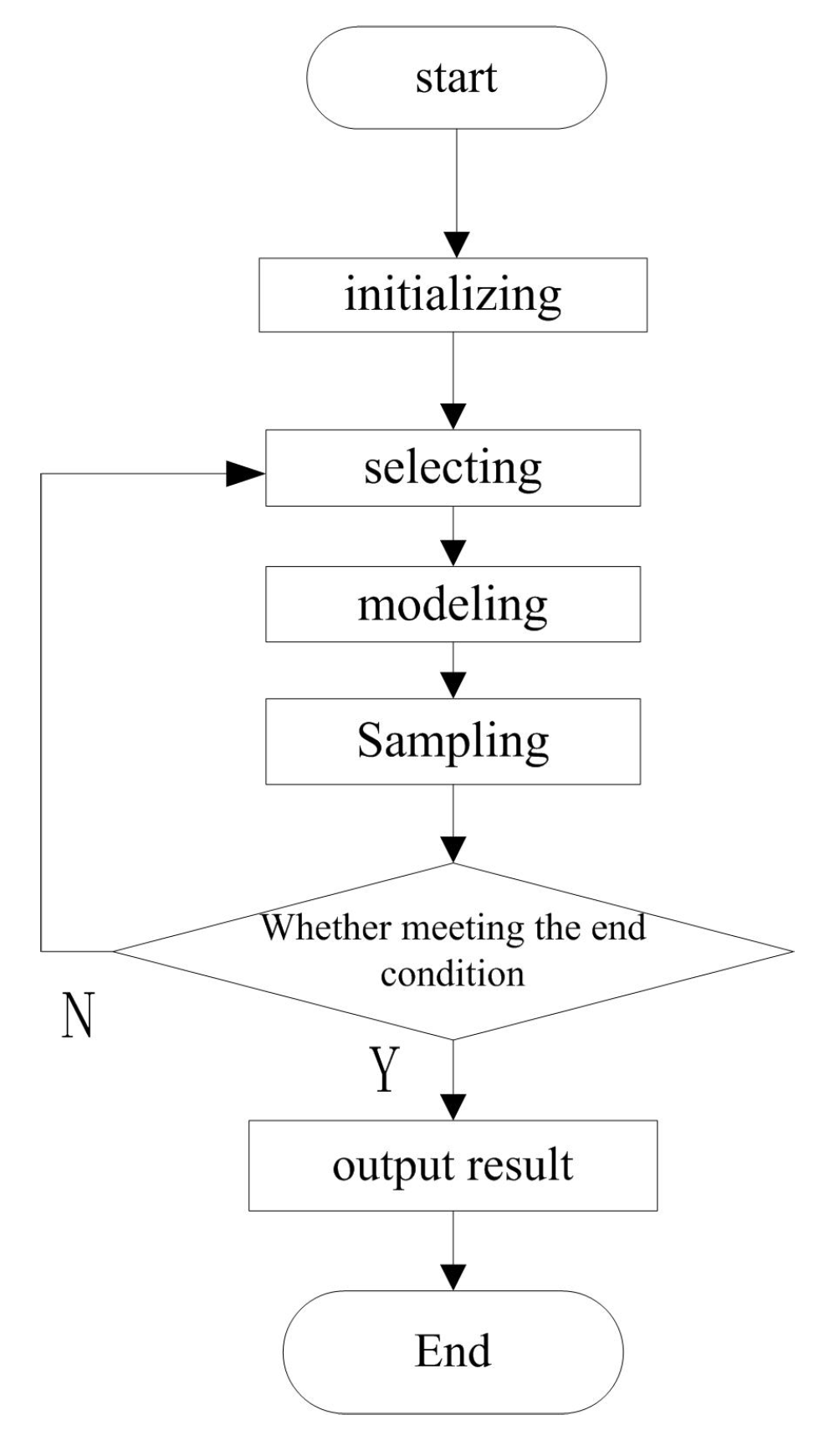
3.1. Estimation of Distribution Algorithm

The idea of EDA originates from genetic algorithm, but it is different from genetic algorithm. The genetic algorithm is a kind of searching method, which simulates the natural evolution at the micro level, while the EDA controls algorithm search at the macro level [28].
Compared with genetic algorithm, the EDA algorithm does not have crossover and mutation operators. Instead, the two steps of probability modeling and sampling are adopted. The EDA uses the global information of population to establish probability model and control the search procedure of the algorithm from the “micro” level. It has strong global search capability and the ability to solve complex problems of high dimension. In the EDA, a global manipulation mode of operation replaces the genetic operator [29]. The above-mentioned advantages have attracted the interest of many scholars. After more than ten years of development, The EDA algorithm has become a research hotspot in the field of intelligent computation.
The specific implementation steps of the EDA are as follows:
(1)
Initialize the population
(2)
Execute cycle-body
  • Selecting: Select several individuals to form a dominant group according to a certain selection mechanism.
  • Modeling: Establish a probability model according to a certain criteria.
  • Sampling: Use the proposed probability model to generate the next generation; determine whether the termination condition is met. if it is satisfied, output the optimal individual. If not, continue to execute the loop body.
The flow chart of EDA is shown in Figure 1.

3.2. The Principle of Bayesian Statistical Inference

The key to the EDA algorithm is how to establish and update the probability model reasonably and efficiently. The main feature of Bayesian statistical inference is the use of prior distribution. After getting the sample observation values, the posterior distribution is obtained from the information provided by the sample observations and the prior distribution by [30]. The posterior distribution which contains abundant information is the basis for Bayesian statistical inference. Due to the application of prior distribution, Bayesian statistical inference has a good statistical inference effect on both large and small samples. A typical Bayesian formula is:
q A i / B = q A i q B / A i j = 1 n q A i q B / A i
where, event A 1 , A 2 , , A n are complete event group. i = 1 , 2 , , n ; q A i is the prior distribution probability model. And the occurrence of event B can affect the probability of occurrence of event A 1 , A 2 , , A n . Therefore, it needs to be re-estimated. Finally, it is expressed in the form of the posterior distribution.
Therefore, the Bayesian inference model uses the prior information and the actual sample information to obtain the posterior information and it transforms the prior distribution into the posterior distribution, which forms the Bayesian statistical inference model.

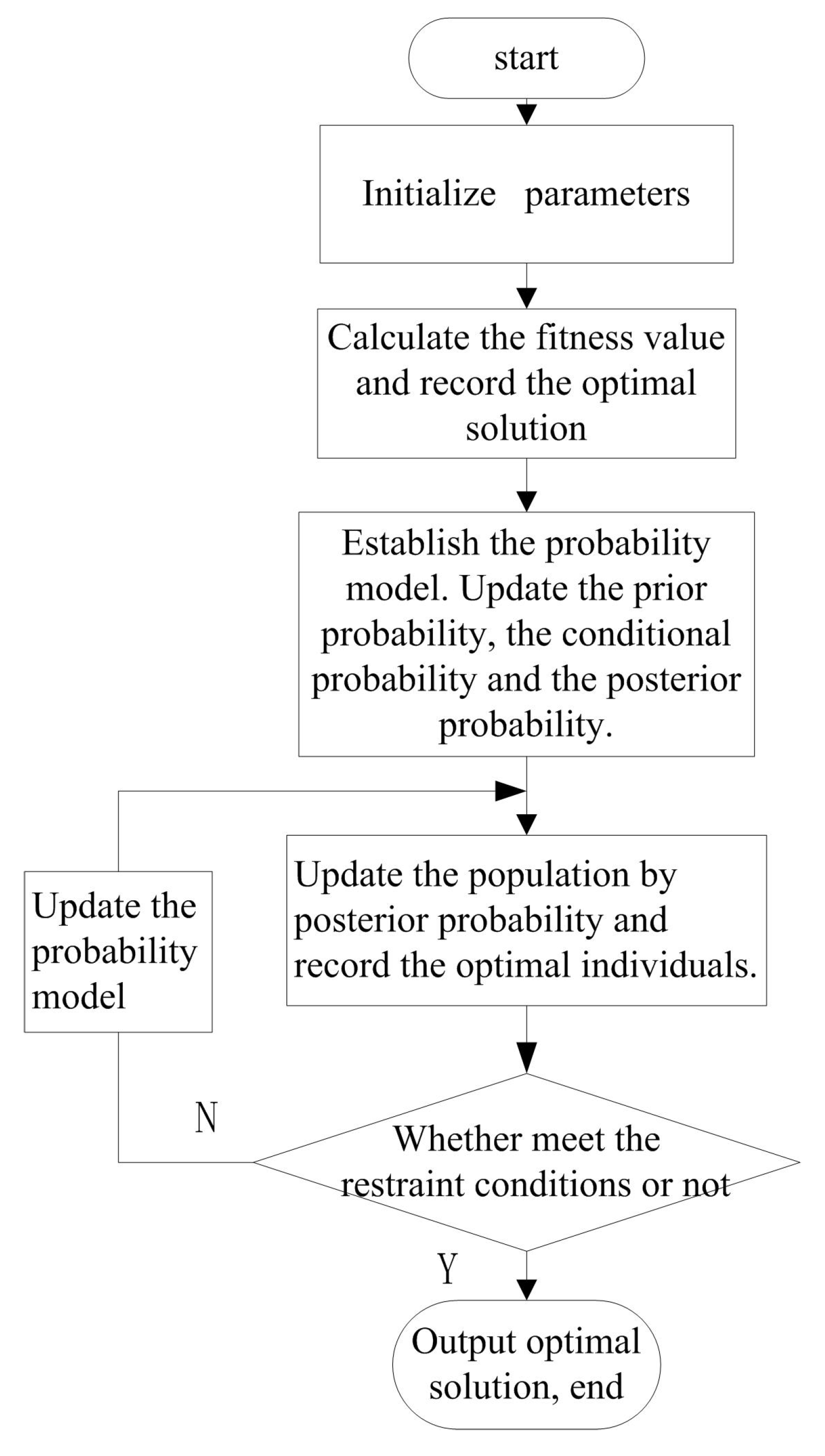
3.3. The EDA with Bayesian Inference Improved

3.3.1. Establishment of IEDA Probability Model

In the multivariate related discrete optimization problem, the position or value of each variable in the individual directly affects the individual’s fitness. Therefore, establishing a probability model that reflects the value of each variable is the key to solving such problems in the EDA . The probability model established by Bayesian inference includes three models: prior probability, conditional probability and posterior probability.
(1) Establishment of prior distribution probability model
The individual variables in the EDA algorithm in this paper are binary coded. Set the individual length to be l. X = x 1 , x 2 , , x l represents an individual. And x j is a variable in the jth position. Establish a prior distribution probability for variables at each position. The prior probability of all variables composed a prior distribution probability model:
q x = q 1 , q 2 , , q l T
(2) Establishment of conditional distribution probability model
q y t = q t x t * 1 / x t 1 q t x t * 1 / x t 1 q t x t * l / x t 1 q t x t * 1 / x t 2 q t x t * 2 / x t 2 q t x t * l / x t 1 q t x t * 1 / x t l q t x t * 2 / x t l q t x t * l / x t l
Each variable in an individual will affect other variables, Therefore, a conditional probability vector can be used to indicate the influence of the remaining variables on the variable x j , which can be expressed as q j = q x j / x 1 , q x j / x 2 , , q x j / x l T . The conditional probability can be obtained according to individual information in the dominant group, which characterizes the conditional probability of variable x j when other variables take a certain value. Assuming the following conditions, the k t h individual in the dominant group is represented as X k t = x k t 1 , x k t 2 , , x k t l while the winning individual in the t t h generation is X t * = x t * 1 , x t * 2 , , x t * l in the tth generation. we can establish the conditional matrix q y t of the t t h generation according to the winning individuals and dominant groups. And the conditional matrix is shown in Formula (7).
According to statistical theory:
q t x t * j / x t i = q t x t * j · x t i / q t x t i
where, q t x t * j · x t i represent the probability when the variable x j in the winning individual and the variable x i in the dominant group take the specific value at the same time. And q t x t i represent the probability when variable x i takes a specific value in the dominant group.
(3) Establishment of posterior distribution probability model
When the population evolves to the t t h generation, the corresponding conditional probability matrix is q y t . By using the prior probability and the conditional probability, the posterior probability model q h t : { q i j t = q t i / x t * j , i , j = 1 , 2 , , l } is established according to the Bayesian formula.
q t i / x t * j = q t x t * j / x t i · q i t / i l q t x t * j / x t i · q i t
where, the denominator is the sum product of the j t h column of the prior probability and the conditional probability matrix. It portrays the conditional probability of re-estimating the value of other variables under the condition that the corresponding variable of the optimal individual takes a specific value. The posterior probability matrix q y t combines the prior information and the new information provided in the evolutionary process, so it has better statistical inference results.

3.3.2. Update of Probability Model

The posterior distribution probability model is obtained through calculation of the prior distribution probability model and conditional distribution probability model. Therefore, the update of the probability model can be divided into two steps. First, updating the prior distribution probability model and the conditional probability model, and then combining the updated information of the two model to obtain an updated posterior distribution probability model.
(1) Update of prior distribution probability model
When the population evolve to the t t h generation, and the winning individuals is X t * = x t * 1 , x t * 2 , , x t * l . According to the information of the individuals in the dominant group D t , the updated prior distribution probability is as follows:
q j t + 1 = 1 α m k = 1 m δ j t k q j t + α m k = 1 m δ j t k x k t j = x k t * j 1 α m k = 1 m δ j t k q j t x k t j x k t * j
δ j t = 1 x k t j = x k t * j 0 x k t j x k t * j
where, the value of δ j t j = 1 , 2 , , l is related to the value of the corresponding position of the individuals in the dominant group and the winning individuals. If the two are equal, the value take 1, if not, take 0. α is a control parameter between (0, 1), and the larger α is, the greater the influence is implemented on the offspring. And m is the number of individuals in the dominant group.
(2) Update of conditional distribution probability model
The update of conditional distribution probability model should be carried out through the information of the dominant group D t , which can be formulated as follows:
q a , b t + 1 = 1 β q a , b t + β m k = 1 m λ a , b t
λ a , b t = 1 T h e v a r i a b l e a a n d b a r e a l l 0 0 o t h e r
where, q a , b t + 1 is an element in the conditional probability matrix model. a = b = 1 , 2 , , l , β 0 , 1 m parameter is the same as above. t is an evolutionary algebra of the current dominant group. The function of the controlling parameter β is similar to that of α .
(3) Update the probability model of posteriori distribution
Using the updated prior distribution probability model and conditional distribution probability model, a new posterior probability model can be obtained by Bayesian formula.

3.3.3. Population Regeneration

New individuals are generated based on the updated posterior probability model. The sampling method is setting each column of the updated posterior probability as basis, and adopting the roulette wheel selection repeatedly to select the value of each position and then produce a new individual, The new individual, together with the current dominant population, consist of the next generation. Then calculate the fitness of the new individual and judge the convergence.

3.4. Algorithm Steps

The flow chart of solving the distributed generation optimization configuration problem of the IEDA is shown in Figure 2. Use the Formula (1) as fitness function, the algorithm steps are as follows:
Step 1: Individual coding. Take the capacity of the distributed generation connected to each bus of the radial distribution system as a variable. l buses corresponds to the l variables, Therefore, the dimension of the individual X is l. That is, one solution vector of the system is X = x 1 , x 2 , , x l . Each variable can only be 0 or a non-zero constant C. A variable equals 0 means that the bus is not connected to the distributed generation. That the variable value is a non-zero constant C indicates that the bus is connected to the distributed power source, and C is the capacity of the access.
Step 2: Generate the initial population. Arrange a certain number of zero in the position of all variables randomly to form the initial population, which can be stored in the initial group N(d) if the network topology analysis meets the requirements.
Step 3: Calculate the fitness and choice of dominant groups. Calculate the individual fitness by the fitness function, and select a certain proportion of dominant individuals from the group to form the dominant group D(m). The selection rate M is determined by the size of initial population.
Step 4: Establish probability model based on dominant group. After establishing a priori distribution probability model, a conditional probability model and a posteriori probability model is formed through proportional selection. Update the prior probabilities and conditional probabilities according to the superior individuals and groups in D(m), and then update the posterior probability according to the updated priori probabilities and conditional probability.
Step 5: Generate new individuals by sampling from the posterior probability model. The updated posterior probability model is sampled through the roulette wheel selection to generate new individuals and calculate fitness. With the increase of evolutionary algebra, the probability of the emergence of the optimal individual increases gradually. When the probability reaches a certain value, the calculation would be terminated, and then the optimal solution is optimum individual in the current dominant group. Otherwise, a new dominant group is selected from the population and the step 6 is executed.
Step 6: Update the probability model, return to step 5, repeat the above steps until the terminating conditions are satisfied.

4. Load Flow Analysis

Distribution load flow is an important part of distribution automation system and distribution management system. The solution of the network reconfiguration, reactive power optimization and state estimation problem require efficient power flow calculation methods. Due to the High-impedance ratio of the distribution system, the fast decoupling and Newton Raphson load method is not suitable for the calculation of the load of the distribution system. Therefore, this paper uses a direct solution method to calculate the power flow of distribution network and get a better solution. Using two developed matrices, the bus-injection to branch-current matrix and the bus-current to bus-voltage matrix and a simple matrix multiplication are used to obtain load flow solutions [31].
For distribution networks, the expression for S i is
S i = P i + Q i , i = 1 , 2 , , N
where N is the number of buses, P i is the active power of bus i, and Q i is the reactive power of bus i. The injection current is calculated as follows:
I i = S i / V i *
The relationship between the injected bus current and the bus voltage is expressed as follows:
Δ V = B C B V B I B C I = D L F I
where BCBV is the branch–current to bus–voltage matrix. BIBC is the bus–injections to branch–currents matrix.
The solution to the load of radial distribution system can be obtained with Equations (17)–(19).
I i k = S i / V i k *
Δ V k + 1 = D L F I k
V k + 1 = V 0 Δ V k + 1

5. Power Calculation

The power is calculated by a set of simplified recurrence equations.
P i + 1 = P i P L i + 1 R L i + 1 × P i 2 + Q i 2 V i 2
Q i + 1 = Q i Q L i + 1 X L i + 1 × P i 2 + Q i 2 V i 2
where P i and Q i are the active and reactive power of bus i, and P L i and Q L i are the active and reactive load powers on bus i, respectively. The resistance and reactance of line parts between bus i and i + 1 are represented by R l i + 1 and X l i + 1 , respectively. The power loss of the line part of the bus i and i + 1 can be calculated as follows:
P L o s s i , i + 1 = R L i + 1 × P i 2 + Q i 2 V i 2
Q L o s s i , i + 1 = X L i + 1 × P i 2 + Q i 2 V i 2
The active, reactive and total power losses of the distribution system can be determined by summarizing the losses of all the lines in the distribution system.
P T , L o s s = B I B C × P L o s s i , i + 1
Q T , L o s s = B I B C × Q L o s s i , i + 1
T L o s s = P T , L o s s 2 + Q T , L o s s 2

6. Case Studies

In order to evaluate the proposed algorithm, simulations implemented in 12 bus, 34 bus and 69 bus systems. The result of proposed algorithm is compared with that of the EDA and the GA. The initialization of parameters is as follows: the probability update control factor α = β = 0.25 , the number of individuals in the initial population s = 100 , and the dominant population selection rate M = 0.4 .

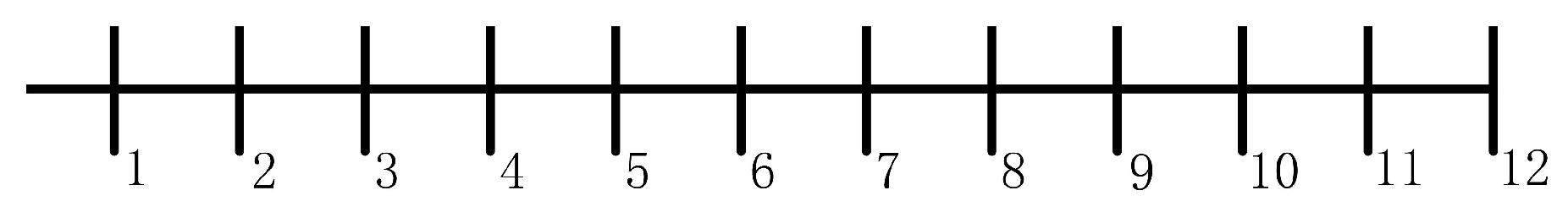
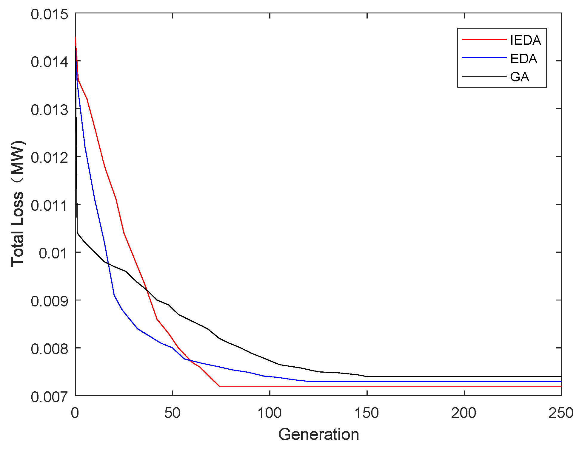
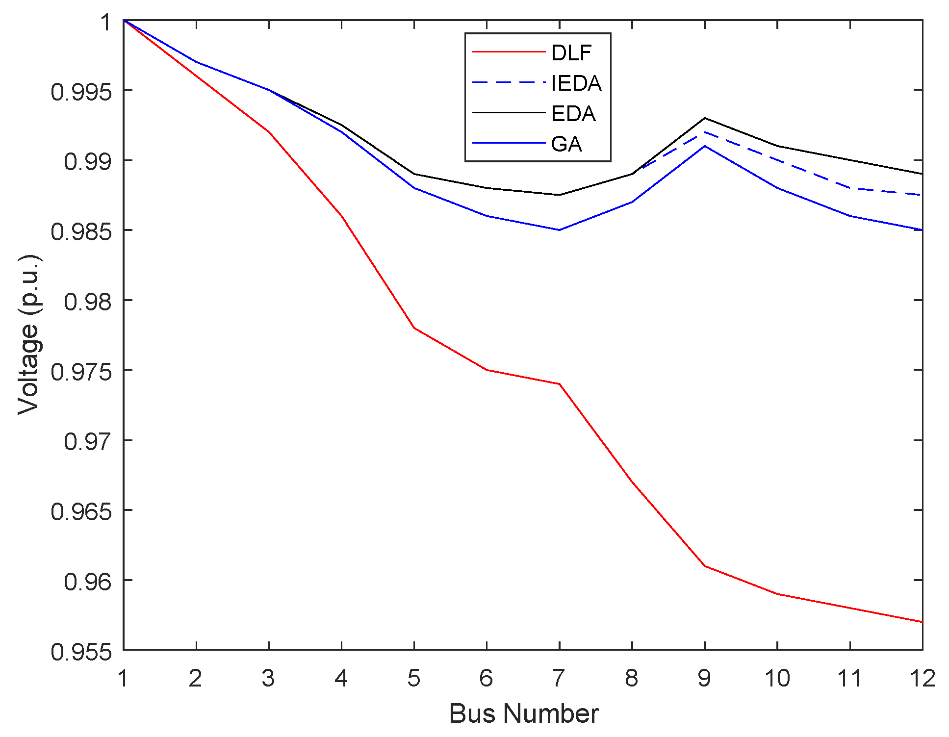
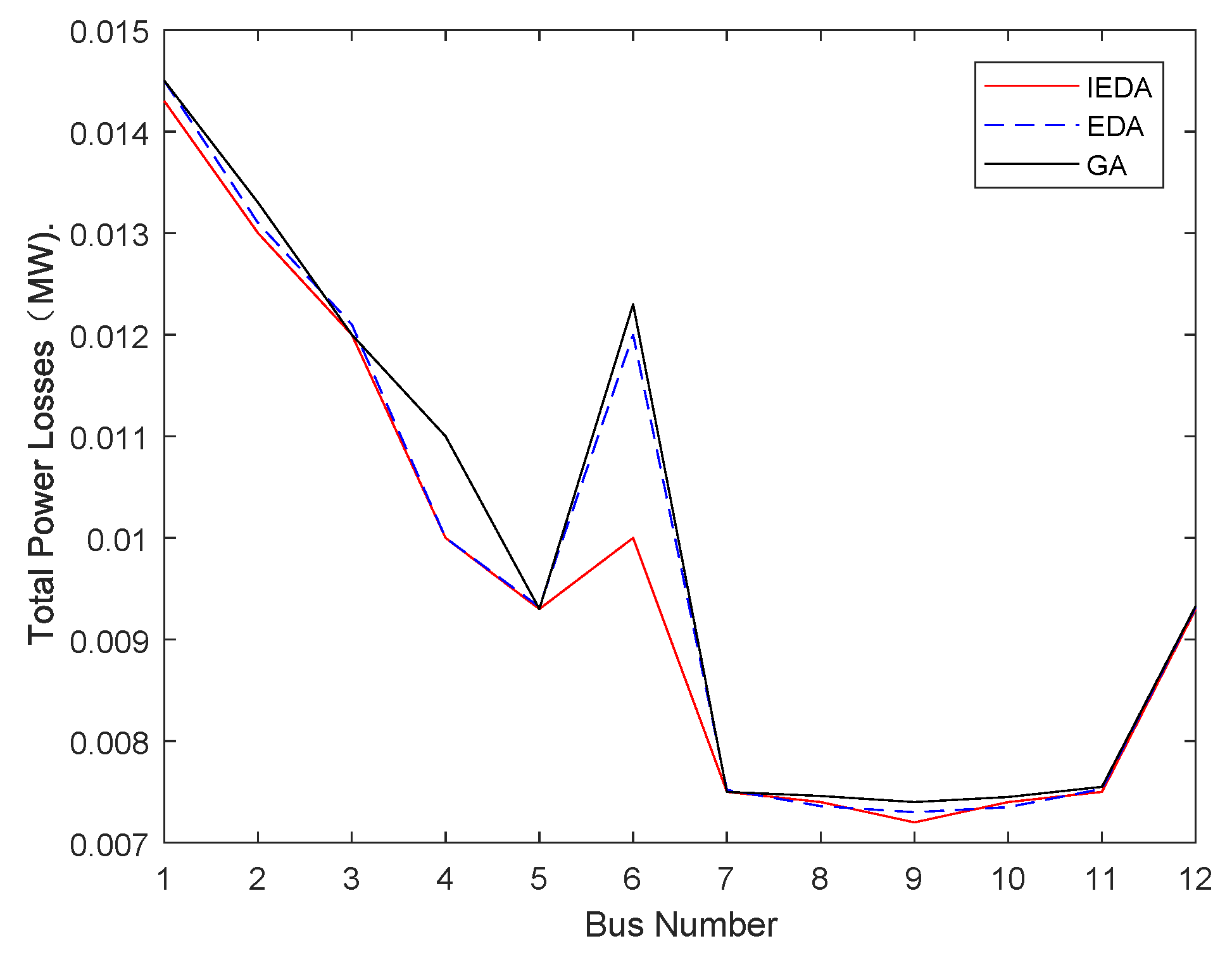
6.1. Test System 1: 12 Bus Radial Distribution System

As shown in Figure 3, the test system consists of 12 buses and 11 branches. The total active load and total reactive load of the system are 0.4350 MVA and 0.390 MVAR. IEDA, EDA and GA are applied to DG optimal configuration problem. Figure 4 is the convergence curve of the No. 9 bus network loss optimization in the 12 bus radial distribution system obtained by IEDA, EDA and GA respectively. It is shown in the graph that the convergence rate of the IEDA is the fastest. After 70 iterations, the loss value of the network is almost converged. The convergence speed of EDA and GA is much slower than IEDA and GA. EDA iterate 120 times to stabilize and GA iterate 150 times to stabilize. In terms of network loss, IEDA is also more competitive than other algorithms. The best result obtained by IEDA is 0.0072 which is smaller than EDA’s 0.0073 and GA’s 0.0074.
Figure 5 is the voltage distribution of the 12 bus radial distribution system with the adoption of IEDA, EDA and GA respectively. Figure 6 is the power losses distribution of the 12 bus radial distribution system. From the graph, we can draw the conclusion that the No. 9 bus has the lowest power loss. As shown in Table 2, the best location of DG in the 12 bus radial distribution systems is the No. 9. The best result obtained by IEDA, EDA and GA is 0.2335 MW, 0.2378 MW and 0.2385 MW, respectively. Therefore, the improved algorithm has the fastest convergence speed as well as the best optimization results. Without changing the DG access capacity, this improved algorithm can obtain better results.

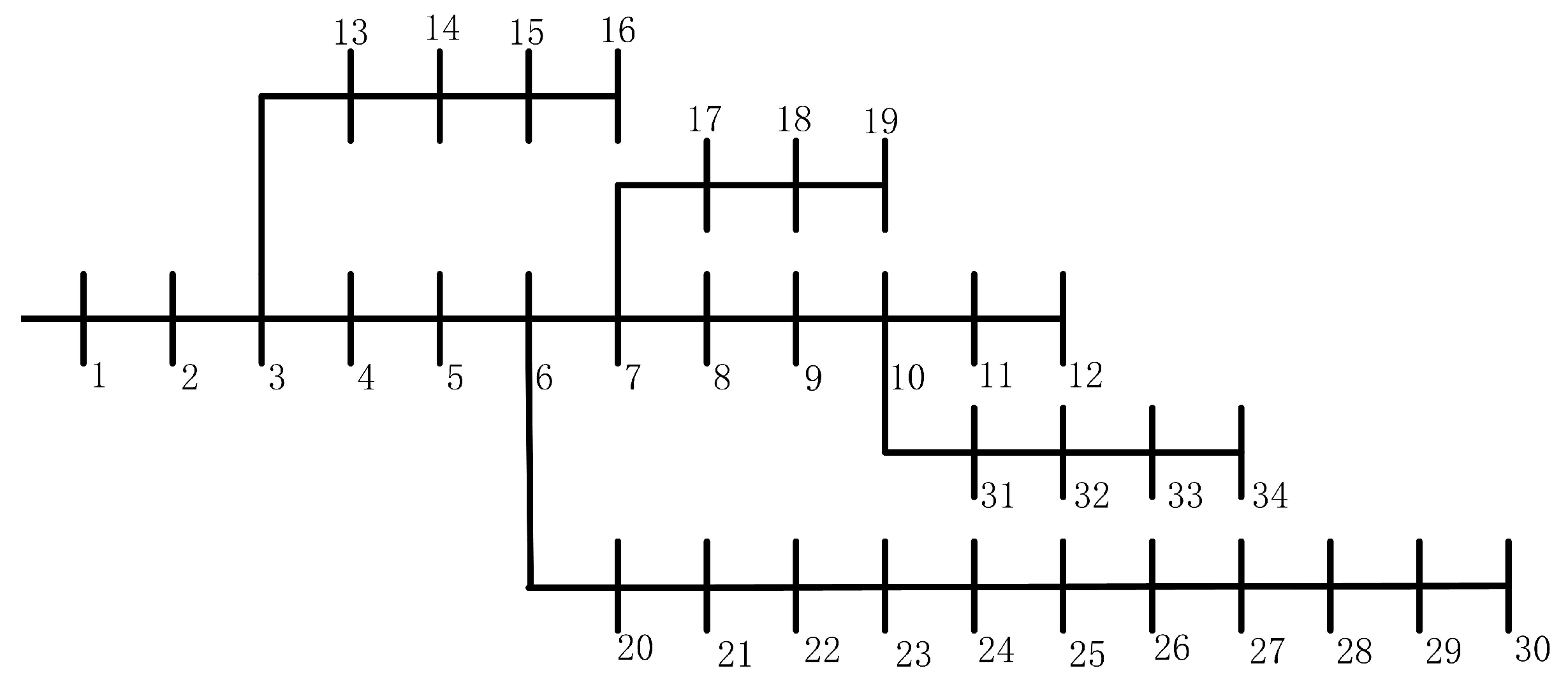
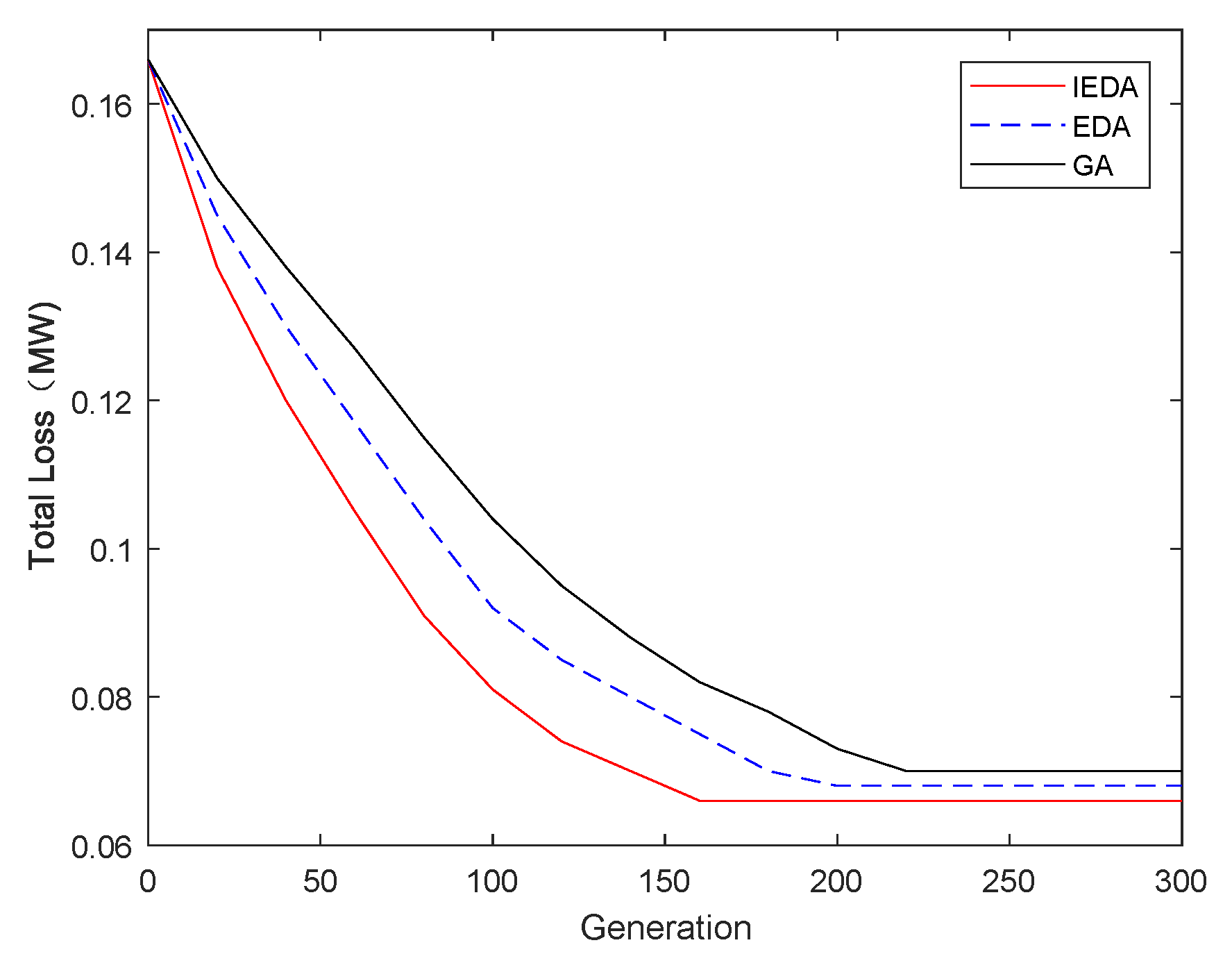
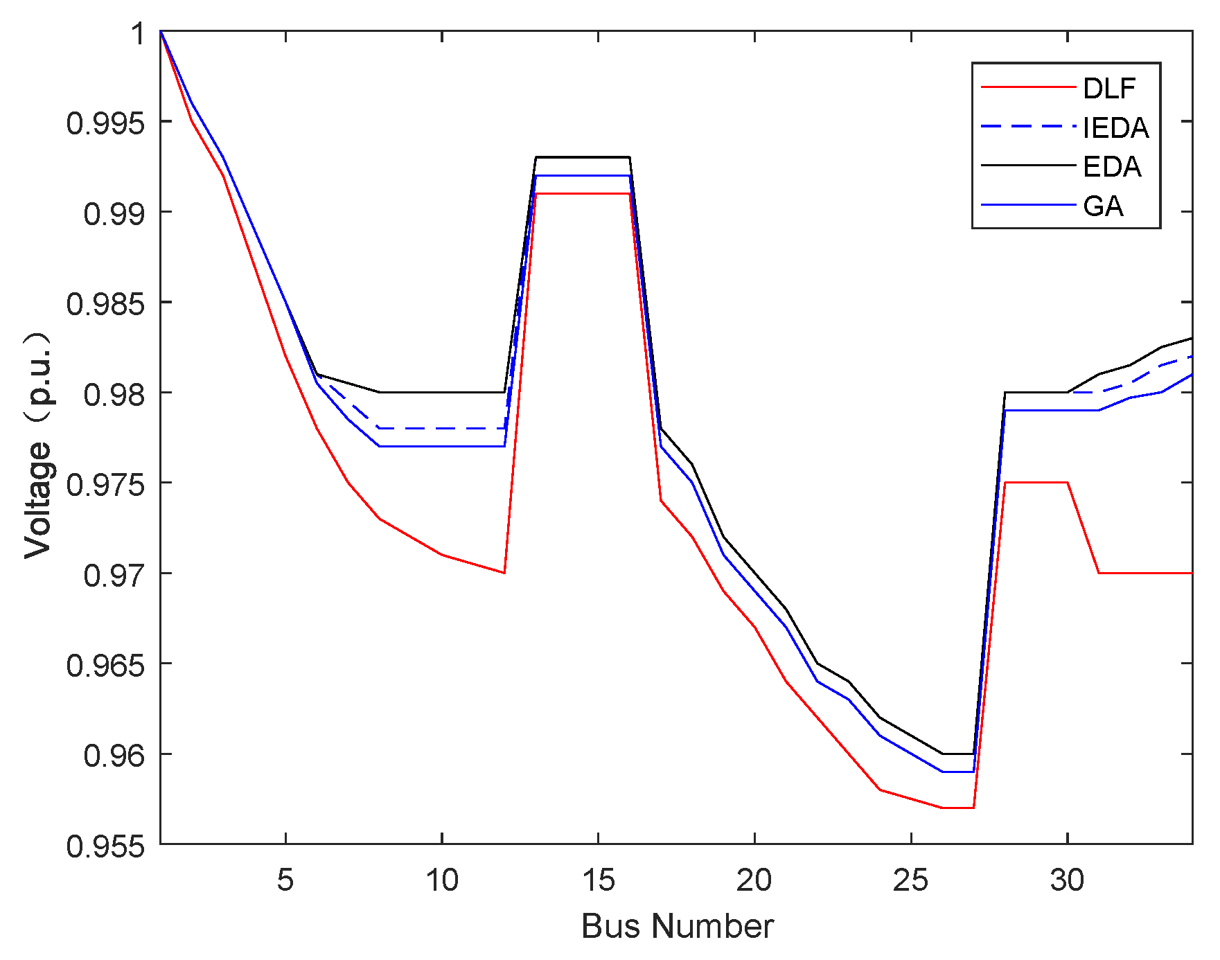
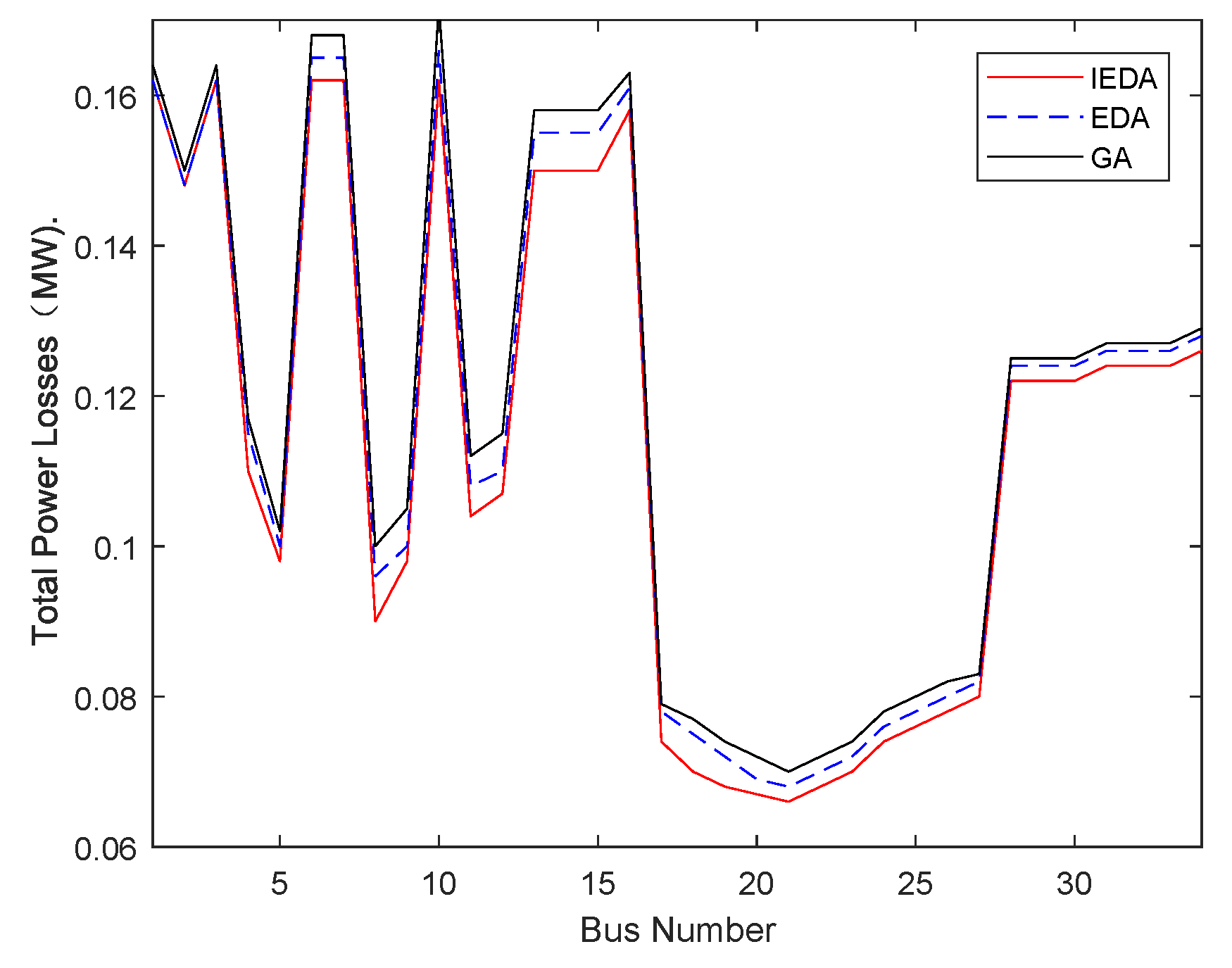
6.2. Test System 2: 34 Bus Radial Distribution System

As shown in Figure 7, the test system consists of 34 buses and 33 branches. The total active load and total reactive load of the system are 4.6365 MVA and 2.8735 Mvar, respectively. Taking the minimization of total power loss as the objective function, IEDA, EDA and GA are used to locate and size the DG. Figure 8 is the convergence curve of the No. 21 bus network loss optimization in the 34 bus radial distribution system obtained by IEDA, EDA and GA respectively. It is shown in the graph that the convergence rate of the IEDA is the fastest. After 160 iterations, the loss value of the network is converged. The convergence speed of EDA and GA is much slower than IEDA and GA. EDA iterate 200 times and GA iterate 220 times before their convergence. In terms of network loss, IEDA is also more competitive than other algorithms. The best result obtained by IEDA is 0.066 which is smaller than EDA’s 0.068 and GA’s 0.07.
Figure 9 is the voltage distribution of the 34 bus radial distribution system with the adoption of IEDA, EDA and GA respectively. Figure 10 is the power losses distribution of the 34 bus radial distribution system. From the graph, we can draw the conclusion that the No. 21 bus has the lowest loss. It can be seen from Table 2 that the best location of DG in the 34 buses radial distribution systems is the No. 21 The best result obtained by the IEDA, EDA and GA is 2.9506 MW, 3.0023 MW and 3.0112 MW respectively. Therefore, the improved algorithm has the fastest convergence speed as well as the best optimization results. Without changing the DG access capacity, this improved algorithm can obtain better results.

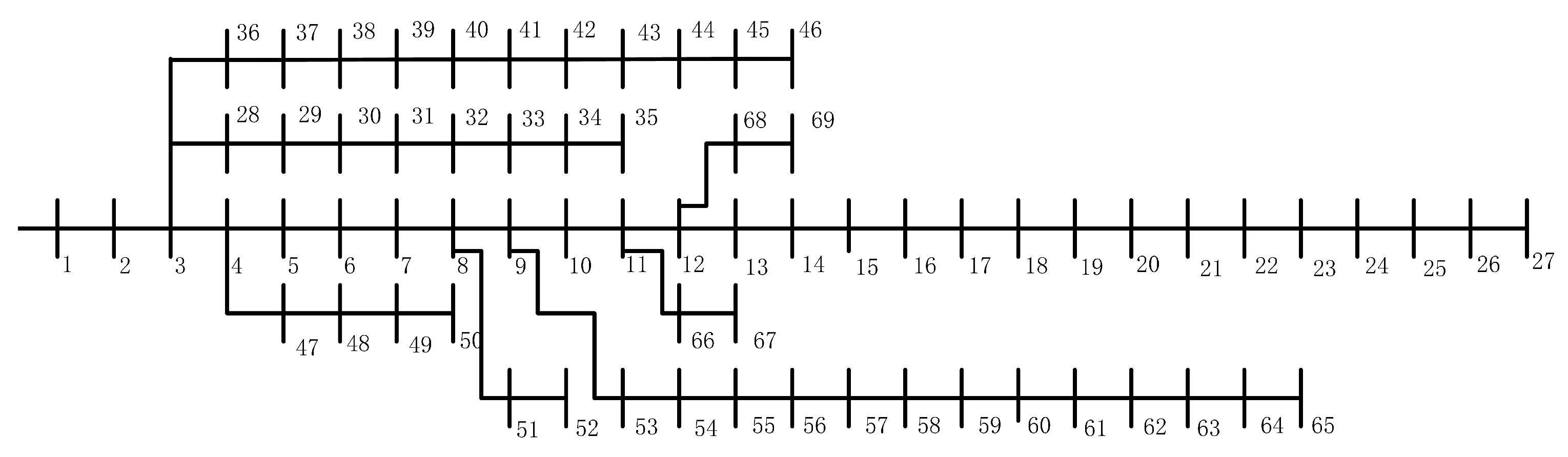
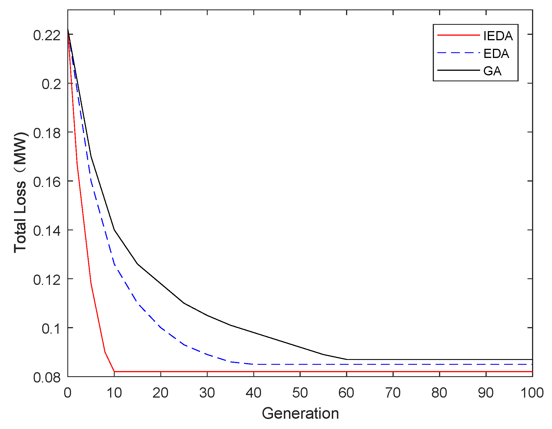
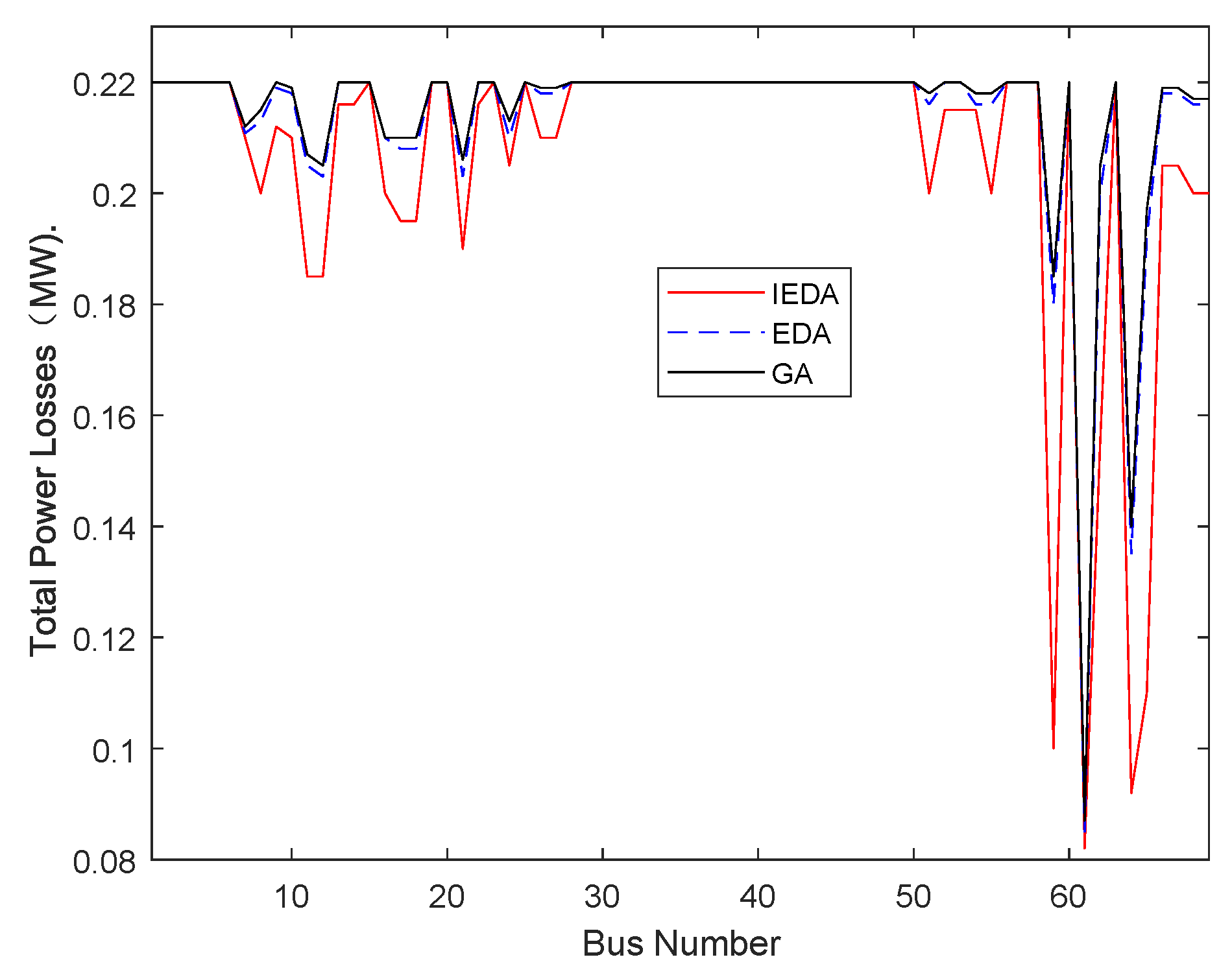
6.3. Test System 3: 69 Bus Radial Distribution System

As shown in Figure 11, the test system consists of 69 buses and 68 branches. The total active load and total reactive load of the system are 3.8021 MVA and 2.6945MVAR, respectively. Taking the minimization of total power loss as the objective function, IEDA, EDA and GA are used to locate and size the DG respectively. Figure 12 is the convergence curve of the No. 61 bus network loss optimization in the 69 bus radial distribution system obtained by IEDA, EDA and GA respectively. It is shown in the graph that the convergence rate of the IEDA is the fastest. After 10 iterations, the loss value of the network is basically stable. EDA and GA converge appear to be much slower, EDA iterate 40 times to stabilize and GA iterate 60 times to stabilize. In terms of network loss, IEDA is also more competitive than other algorithms. The best result obtained by IEDA is 0.082 which is smaller than EDA’s 0.085 and GA’s 0.087.
Figure 13 is the voltage distribution of the 69 bus radial distribution system with the adoption of IEDA, EDA and GA respectively. Figure 14 is the bus losses distribution of the 69 bus radial distribution system. From the graph, we can draw the conclusion that the No. 61 bus has the lowest loss. It can be seen from Table 2 that the best location of DG in the 69 bus radial distribution systems is the No. 61 bus The best result obtained by the IEDA, EDA and GA is 1.8705MW, 2.0661MW and 2.0845MW respectively. Therefore, the improved algorithm has the fastest convergence speed as well as the best optimization results. Without changing the DG access capacity, this improved algorithm can obtain better results.

7. Conclusions

In this paper, Bayesian statistical-inference with distribution estimation creates a powerful optimization algorithm known as IEDA which reduces the total power loss and improves the voltage profile with proper allocation and sizing of DG. The global search ability of EDA algorithm is outstanding. Combined with Bayesian statistical reasoning, it can improve its convergence speed. EDA, GA and IEDA generate solutions which satisfy all the equality and inequality constraints. However, IEDA converges faster when compared to EDA and GA. The practical application and efficacy of this method was evaluated using three various common test systems (12, 34, and 69 bus). The comparative analysis of EDA, GA and IEDA methods for optimal placement and sizing of DG in a distribution system to minimize the total real power loss was successfully done. From the results, it is concluded that IEDA algorithm gives better results than EDA algorithm and GA algorithm, in terms of its accuracy and convergence speed. However, the optimum placement is identical to EDA and GA algorithms. IEDA algorithm can minimizes the real power loss simply and quickly without any complex calculations. Thus, the results obtained pave the way for new and promising research area, utilizing EDA algorithm with improvement, giving better results with high convergence speed.
In the future, to reduce the computational burden further optimal DG placement can be done by any of the recent methods such as sensitivity analysis, voltage stability consideration, loss sensitivity factor, etc. and the sizing can be done with IEDA.

Author Contributions

Conceptualization, L.Y.; Methodology, Y.W.; Project administration, X.Y.; Supervision, X.Y., Y.W. and X.L.; Validation, L.Y. and Y.W.; Writing–original draft, L.Y.; Writing–review and editing, X.Y.

Acknowledgments

This work was supported in part by the National Natural Science Foundation of China (51765042, 61463031, 61773051 and 61662044), Jiangxi Provincial Department of Science and Technology (JXYJG-2017-02), Jiangxi Natural Science Foundation (20171ACB20007) and Jiangxi Provincial Department of Science and Technology (20121BBE50023 and 20133BCB22002).

Conflicts of Interest

The authors declare no conflict of interest.

Nomenclature

DGDistributed generation
IEDAImproved estimation of distribution algorithm
EDAEstimation of distribution algorithm
GAGenetic algorithm
T L o s s The total power loss of the radial distribution system
P D G i The real power generation using DG at bus i
P D i The power demand at bus i
P L o s s The line loss on the bus i
U i m i n The lower limits of voltages at bus i
U i m a x The upper limits of voltages at bus i
I i m a x The maximum current value of branch i
S i The apparent power of bus i
P i The active power of bus i
Q i The reactive power of bus i
BCBVThe branch–current to bus–voltage matrix
BIBCThe bus–injections to branch–currents matrix
P L i The active load powers on bus i
Q L i The reactive load powers on bus i

References

  1. Cano, E.B. Utilizing fuzzy optimization for distributed generation allocation. In Proceedings of the TENCON 2007 IEEE Region 10 Conference, Taipei, Taiwan, 30 October–2 November 2007; pp. 1–4. [Google Scholar]
  2. Keane, A.; Ochoa, L.F.; Borges, C.L.; Ault, G.W.; Alarcon-Rodriguez, A.D.; Currie, R.A.; Pilo, F.; Dent, C.; Harrison, G.P. State-of-the-art techniques and challenges ahead for distributed generation planning and optimization. IEEE Trans. Power Syst. 2013, 28, 1493–1502. [Google Scholar] [CrossRef]
  3. Naderi, E.; Seifi, H.; Sepasian, M.S. A dynamic approach for distribution system planning considering distributed generation. IEEE Trans. Power Deliv. 2012, 27, 1313–1322. [Google Scholar] [CrossRef]
  4. Peng, X.; Lin, L.; Zheng, W.; Liu, Y. Crisscross optimization algorithm and monte carlo simulation for solving optimal distributed generation allocation problem. Energies 2015, 8, 13641–13659. [Google Scholar] [CrossRef]
  5. Devi, S.; Geethanjali, M. Application of modified bacterial foraging optimization algorithm for optimal placement and sizing of distributed generation. Expert Syst. Appl. 2014, 41, 2772–2781. [Google Scholar] [CrossRef]
  6. Sheng, W.; Liu, K.Y.; Liu, Y.; Meng, X.; Li, Y. Optimal placement and sizing of distributed generation via an improved nondominated sorting genetic algorithm II. IEEE Trans. Power Deliv. 2015, 30, 569–578. [Google Scholar] [CrossRef]
  7. Prakash, P.; Khatod, D.K. Optimal sizing and siting techniques for distributed generation in distribution systems: A review. Renew. Sustain. Energy Rev. 2016, 57, 111–130. [Google Scholar] [CrossRef]
  8. Aman, M.; Jasmon, G.; Mokhlis, H.; Bakar, A. Optimal placement and sizing of a DG based on a new power stability index and line losses. Int. J. Electr. Power Energy Syst. 2012, 43, 1296–1304. [Google Scholar] [CrossRef]
  9. Gitizadeh, M.; Vahed, A.A.; Aghaei, J. Multistage distribution system expansion planning considering distributed generation using hybrid evolutionary algorithms. Appl. Energy 2013, 101, 655–666. [Google Scholar] [CrossRef]
  10. Hung, D.Q.; Mithulananthan, N.; Bansal, R. Analytical strategies for renewable distributed generation integration considering energy loss minimization. Appl. Energy 2013, 105, 75–85. [Google Scholar] [CrossRef]
  11. Acharya, N.; Mahat, P.; Mithulananthan, N. An analytical approach for DG allocation in primary distribution network. Int. J. Electr. Power Energy Syst. 2006, 28, 669–678. [Google Scholar] [CrossRef]
  12. Keane, A.; O’Malley, M. Optimal utilization of distribution networks for energy harvesting. Int. J. Electr. Power Energy Syst. 2007, 22, 467–475. [Google Scholar] [CrossRef]
  13. Peng, X.; Lin, L.; Liu, Y.; Wang, X.; Meng, A. Optimal Dis-tributed Generator Allocation Method Based on Correlation Latin Hypercube Sampling Monte Carlo Simulation Embedded Crisscross Optimization Algorithm. Proc. CSEE 2015, 16, 4077–4085. [Google Scholar]
  14. Atwa, Y.M.; El-Saadany, E.F. Probabilistic approach for optimal allocation of wind-based distributed generation in distribution systems. IET Renew. Power Gener. 2011, 5, 79–88. [Google Scholar] [CrossRef]
  15. Atwa, Y.; El-Saadany, E.; Salama, M.; Seethapathy, R. Optimal renewable resources mix for distribution system energy loss minimization. IEEE Trans. Power Syst. 2010, 25, 360–370. [Google Scholar] [CrossRef]
  16. Gandomkar, M.; Vakilian, M.; Ehsan, M. A genetic–based tabu search algorithm for optimal DG allocation in distribution networks. Electr. Power Compon. Syst. 2005, 33, 1351–1362. [Google Scholar] [CrossRef]
  17. Wang, R.; Li, K.; Zhang, C.; Du, C.; Chu, X. Distributed Generation Planning Based on Multi-Objective Chaotic Quantum Genetic Algorithm. Power Syst. Technol. 2011, 12, 183–189. [Google Scholar]
  18. Yammani, C.; Maheswarapu, S.; Matam, S.K. A Multi-objective Shuffled Bat algorithm for optimal placement and sizing of multi distributed generations with different load models. Int. J. Electr. Power Energy Syst. 2016, 79, 120–131. [Google Scholar] [CrossRef]
  19. Yuvaraj, T.; Devabalaji, K.; Ravi, K. Optimal Allocation of DG in the Radial Distribution Network Using Bat Optimization Algorithm. In Advances in Power Systems and Energy Management; Springer: Berlin, Germany, 2018; pp. 563–569. [Google Scholar]
  20. Seker, A.A.; Hocaoglu, M.H. Artificial Bee Colony algorithm for optimal placement and sizing of distributed generation. In Proceedings of the 2013 8th International Conference on Electrical and Electronics Engineering, Amman, Jordan, 28–30 November 2013; pp. 127–131. [Google Scholar]
  21. Johan, N.F.M.; Azmi, A.; Rashid, M.A.; Yaakob, S.B.; Rahim, S.R.A.; Zali, S.M. Multi-objective using Artificial Bee Colony optimization for distributed generation placement on power system. In Proceedings of the 2013 IEEE International Conference on Control System, Computing and Engineering, Penang, Malaysia, 29 November–1 December 2013; pp. 117–121. [Google Scholar]
  22. Zhao, F.; Si, J.; Wang, J. Research on optimal schedule strategy for active distribution network using particle swarm optimization combined with bacterial foraging algorithm. Int. J. Electr. Power Energy Syst. 2016, 78, 637–646. [Google Scholar] [CrossRef]
  23. Kowsalya, M. Optimal size and siting of multiple distributed generators in distribution system using bacterial foraging optimization. Swarm Evolut. Comput. 2014, 15, 58–65. [Google Scholar]
  24. Chen, Y.; Liu, L.G. Sizing and Locating of Distributed Generations Based on Chaos Particle Swarm Optimization Algorithm. In Applied Mechanics and Materials; Trans Tech Publications: Zurich, Switzerland, 2013; Volume 291, pp. 2119–2123. [Google Scholar]
  25. Jamian, J.J.; Mustafa, M.W.; Mokhlis, H. Optimal multiple distributed generation output through rank evolutionary particle swarm optimization. Neurocomputing 2015, 152, 190–198. [Google Scholar] [CrossRef]
  26. Dharageshwari, K.; Nayanatara, C. Multiobjective optimal placement of multiple distributed generations in IEEE 33 bus radial system using simulated annealing. In Proceedings of the 2015 International Conference on Circuits, Power and Computing Technologies (ICCPCT-2015), Nagykoyle, India, 19–20 March 2015; pp. 1–7. [Google Scholar]
  27. Popović, Ž.; Kerleta, V.D.; Popović, D. Hybrid simulated annealing and mixed integer linear programming algorithm for optimal planning of radial distribution networks with distributed generation. Electr. Power Syst. Res. 2014, 108, 211–222. [Google Scholar] [CrossRef]
  28. Salhi, A.; Rodríguez, J.A.V.; Zhang, Q. An estimation of distribution algorithm with guided mutation for a complex flow shop scheduling problem. In Proceedings of the 9th Annual Conference on Genetic and Evolutionary Computation, London, UK, 7–11 July 2007; pp. 570–576. [Google Scholar]
  29. Li, D.; Peng, F.; Zhou, X.; Liu, C. Research of Batch Scheduling with Arrival Time Based on Estimation of Distribution Algorithm. In Proceedings of the 2014 Seventh International Symposium on Computational Intelligence and Design, Hangzhou, China, 13–14 December 2014; Volume 2, pp. 125–130. [Google Scholar]
  30. Cai, C.; Yan, G.; Tang, J. Detection of fatigue cracks under environmental effects using Bayesian statistical inference. Int. J. Appl. Electromagn. Mech. 2016, 52, 1015–1021. [Google Scholar] [CrossRef]
  31. Teng, J.H. A direct approach for distribution system load flow solutions. IEEE Trans. Power Deliv. 2003, 18, 882–887. [Google Scholar] [CrossRef]
Figure 1. The flow chart of EDA.
Energies 11 02363 g001
Figure 2. The flow chart of IEDA.
Energies 11 02363 g002
Figure 3. The 12 bus radial distribution system.
Energies 11 02363 g003
Figure 4. Evolution of the fitness function (total loss) with respect to number of generations for bus No. 9 in the 12 bus distribution test system.
Energies 11 02363 g004
Figure 5. Voltage distribution of the 12 bus radial distribution system.
Energies 11 02363 g005
Figure 6. Distribution of network loss of each bus in the 12 bus radial distribution system.
Energies 11 02363 g006
Figure 7. The 34 bus radial distribution system.
Energies 11 02363 g007
Figure 8. Evolution of the fitness function (total loss) with respect to number of generations for bus No. 21 in the 34 bus distribution test system.
Energies 11 02363 g008
Figure 9. Voltage distribution of the 34 bus radial distribution system.
Energies 11 02363 g009
Figure 10. Distribution of network loss of each bus in the 34 bus radial distribution system.
Energies 11 02363 g010
Figure 11. The 69 bus radial distribution system.
Energies 11 02363 g011
Figure 12. Evolution of the fitness function (total loss) with respect to number of generations for bus No. 61 in the 69 bus distribution test system.
Energies 11 02363 g012
Figure 13. Voltage distribution of the 69 bus radial distribution system.
Energies 11 02363 g013
Figure 14. Distribution of network loss of each bus in the 69 bus radial distribution system.
Energies 11 02363 g014
Table 1. Advantages and disadvantages of various algorithms.
AlgorithmAdvantageShortcoming
Analytical methodThe method is simple and less workloadDealing with single objective optimization problem only
Classical optimization algorithmThe model is accurate and the method is simpleThe computation is large and the computation speed is slow
Genetic algorithmThe convergence speed is fast and the versatility is strongIt is more complex, easy to fall into premature convergence, and depends on the initial population
Bat algorithmSimple structure, few parameters and strong robustnessThe speed of convergence is slow and the precision of optimization is low
Artificial bee colony algorithmThe global search ability is strong and the convergence speed is fastit is easy to fall into the local optimum, and the search speed slows down later
Bacterial foraging algorithmStrong parallel search ability and easy to get out of local minimumThe convergence speed is slow and the computation is large
Particle swarm optimizationThe training speed is fast, the efficiency is high, and the algorithm is simpleIt is easy to fall into local optimal solution and poor handling of discrete optimization problems
Simulated annealing algorithmStrong global search capabilityConvergence speed is slow and parallel computing is difficult
Table 2. Test results of various bus radial distribution systems under different algorithms.
Test
System
Total Load
(MVA)
P Loss without
DG (MW)
AlgorithmOptimum Place
(bus no)
Optimum Size
(MW)
P Loss
(MW)
Voltage
(p.u)
IEDA90.23350.00720.992
12 bus0.435 + 0.3900i0.145EDA90.23780.00730.993
GA90.23850.00740.991
IEDA212.95060.0660.968
34 bus4.6365 + 2.8735i0.1638EDA213.00230.0680.969
GA213.01120.0700.967
IEDA611.87050.0820.9815
69 bus3.8021 + 2.6945i0.2254EDA612.06610.0850.9835
GA612.08450.0870.9775

