Physical and Mathematical Modeling of a Wave Energy Converter Equipped with a Negative Spring Mechanism for Phase Control

Abstract

A wave-energy converter has been studied through the combination of laboratory experiments and numerical simulations. The converter model is a semi-submerged axi-symmetric buoy with a circular cross section with a diameter of 26 cm at the water plane. The buoy is pitching about a fixed external axis oriented such that the buoy works primarily in heave. The laboratory model is equipped with a spring mechanism referred to as WaveSpring, which works to shift the resonance period and increase the response bandwidth of the system. A controlled electric actuator was connected and programmed to provide a velocity-proportional force for power extraction. The buoy mass was varied at two levels and the experimental setup was exposed to a selection of regular and irregular waves. The power take-off (PTO) damping was set as a function of sea state. A mathematical model for global motion response was developed based on linear hydrodynamic theory and rigid-body dynamics. Comparison of laboratory measurements and numerical simulation results shows that the dominant physical effects have been well captured by the mathematical model. Overall, the study gives an experimental verification that a negative spring mechanism mounted in parallel with the power take-off machinery of a wave energy converter may be used to increase the average converted power.

1. Introduction

As argued by several authors [1,2,3], some types of wave energy converters will require considerable cycling of mechanical reactive power between motion and machinery in order to absorb and convert ocean wave energy efficiently. Typically, wave energy converters having large hydrostatic stiffness, as found in systems with surface-piercing buoys with vertical or pitching motion, fall into this category. It was recently proposed [4,5] that an arrangement of mechanical springs be used to facilitate this power cycling, such that the power take-off machinery may be designed to handle the active power only. If working at efficiency comparable to or higher than the power take-off machinery, the use of such a mechanism may represent a substantial cost-saving for wave energy units of this type. The cycling of reactive power can then be done with minor losses, ensuring an efficient absorption of wave energy, while the power take-off machinery can be dimensioned according to active power, which is smaller.

Earlier studies [5,6,7] have presented results with theoretical estimates of forces from a negative spring mechanism designed for linear motion. The current paper describes how the same principle may be applied to rotating motion. A laboratory model designed with coil springs is used to demonstrate the effect in practice. The spring mechanism is mounted on a laboratory setup of the WaveStar floater, which has already been studied extensively in other works [8,9]. The reported tests took place in the Deep Water Wave Basin at the Department of Civil Engineering at Aalborg University during two campaigns.

The paper is organized in the following way: First the system configuration and details of the laboratory model is presented in Section 2, and the experimental matrix with all system variations is summarized in Section 4. The mathematical model is described in Section 3, and results from both experiments and simulations are presented and discussed in Section 5.

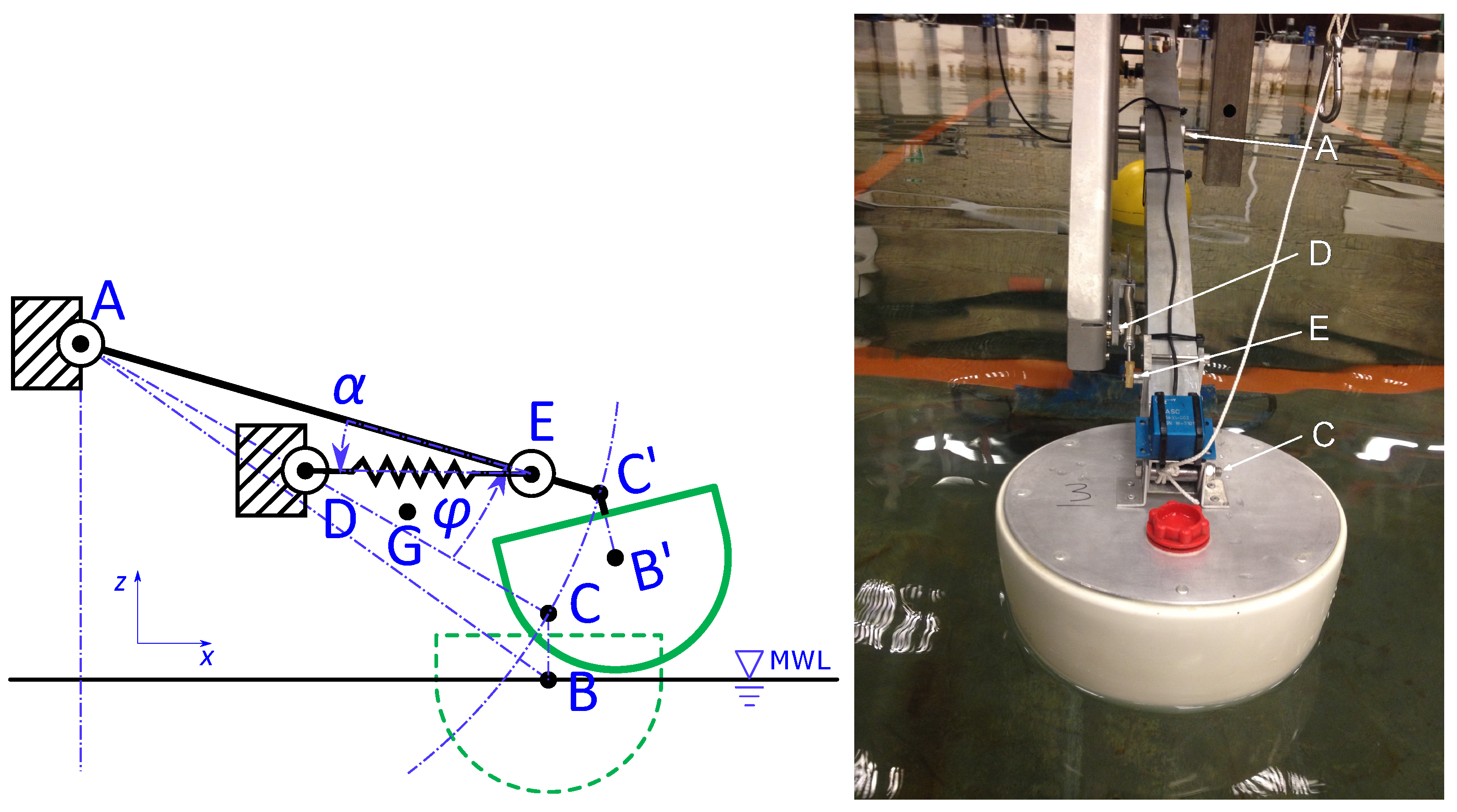
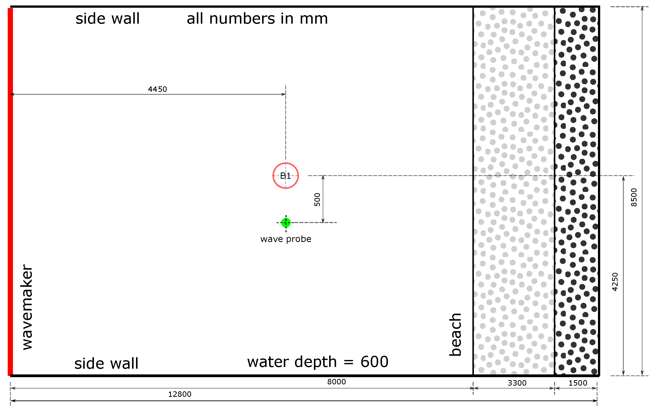
2. Experimental Setup

The physical model used in the present work is shown in Figure 1. It is a 1:20 downscaled buoy of the WaveStar prototype [10]. The buoy may be approximately represented as a hemisphere extended with a cylindrical part on top. It is constrained to rotate about a horizontal axis A fixed at $0.285$ m above the mean water level (MWL). The buoy is connected at point F to a force-controlled LinMot actuator (LinMot Series PS01-37x240, Linmot controller Series E1100), which may be programmed to act as the power take-off (PTO) system of choice. The slider of the actuator is moving with respect to the stator, which is fixed at point L. The force on the system is measured with a load cell (Futek LSB302 300lb) placed between the slider of the actuator and the lever arm of the buoy. A laser-based position sensor (MicroEpsilon ILD-1402-600) follows the position of the slider with respect to the stator. An accelerometer (Analog Devices ADXL203EB) is placed on-top of the buoy enabling a measure of the angle and the angular velocity of the buoy.

Figure 1. Sketch of the physical model of one buoy WaveStar.

The physical model is equipped with a WaveSpring lab model as depicted in Figure 2. A coil spring is fitted between the buoy lever (E) and a fixed point D. The setup was adjusted such that points A, D, and E were found on a straight line when the buoy was at its initial position with the waterline at the top of the hemispherical bottom. When the natural length of the spring exceeds the minimum distance between D and E, the mechanism provides a negative spring force on the buoy’s rotation about its equilibrium position.

Figure 2. Left: Sketch of the WaveSpring assembly fitted to the WaveStar setup. Right: Picture of the WaveSpring model installed on the WaveStar setup in the wave basin.

In order to obtain the contribution of the WaveSpring in terms of moment to the overall system, some governing properties for the WaveSpring laboratory model are listed:

• The spring’s stiffness, k;
• The initial compression force of the spring, which is a function of its natural length $l_0$, its actual length l, and the stiffness k, $F=k(l_0-l)$;
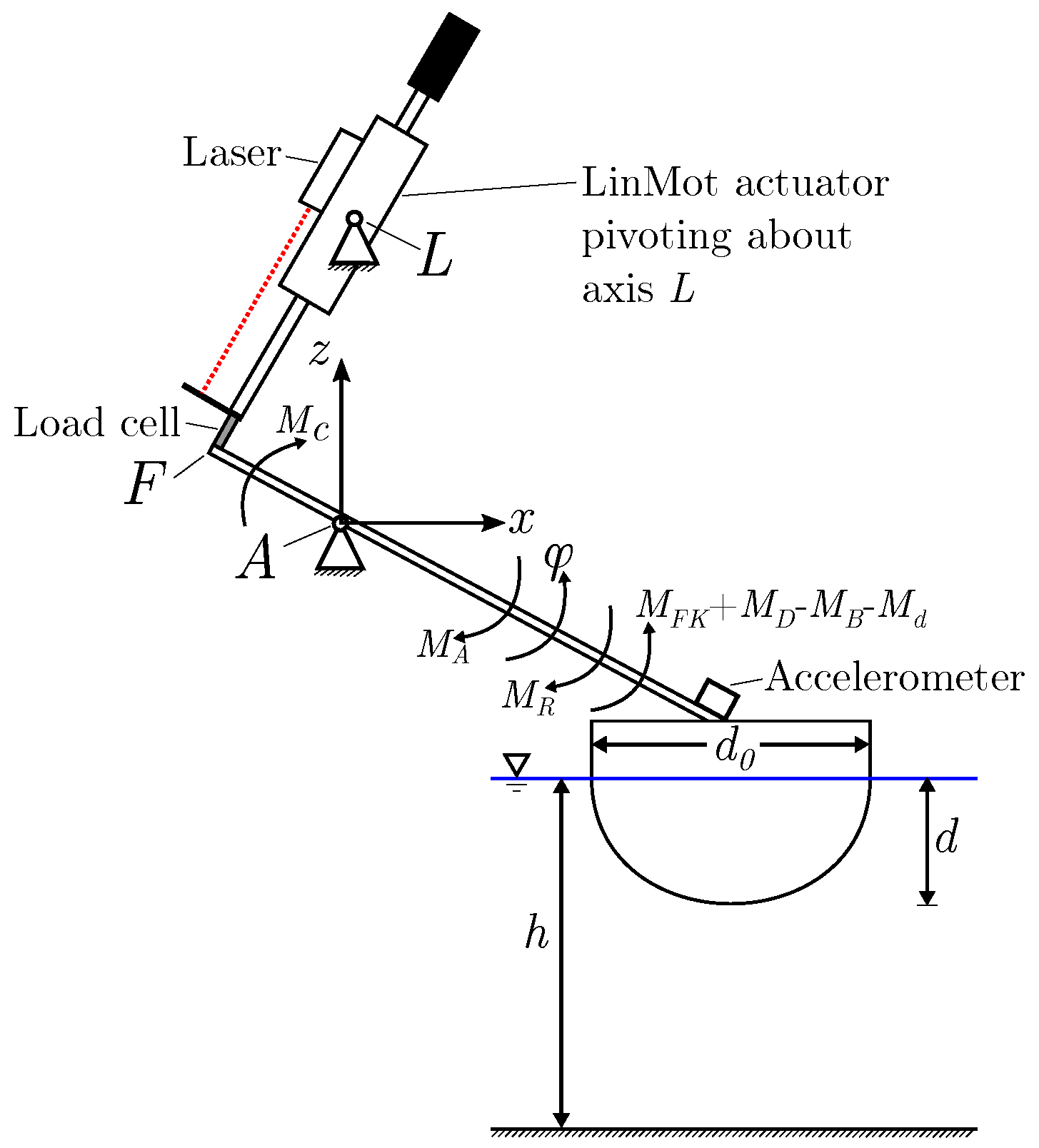
• The angular displacement of $\overline{\mathrm{DE}}$ arm ($\alpha$) as a function of angular displacement of the arm $\overline{\mathrm{AC}}$ axis ($\phi$), cf. Figure 2;
• The change in distance $\overline{\mathrm{DE}}$ as a function of angular displacement of the $\overline{\mathrm{AE}}$ axis ($\phi$).

The two latter properties are governed by the placement of points D and E. Their position are set such that the appropriate negative spring force is achieved over a given range of angular displacement $\phi$. The WaveSpring laboratory model is composed of a coil spring with a stiffness defined as [11]

$$k=\frac{G{d}^4}{8n{D}^3}$$

(1)

where G is the shear modulus, d is the thread diameter, D is the coil diameter, and n is the number of turns.

With the spring dimensions as chosen for the current design, the spring force can be treated as linear. The shear modulus of stainless steel is about 77 GPa.

Let the buoy rotation angle $\phi$ be defined with $\phi =0$ when $\overline{\mathrm{AE}}$ and $\overline{\mathrm{AD}}$ are aligned and with a positive direction for the buoy moving upwards. By geometrical considerations, the length $\overline{\mathrm{DE}}$ may then be expressed as function of $\phi$ in the following way:

$${\overline{\mathrm{DE}}}^2={\overline{\mathrm{AD}}}^2+{\overline{\mathrm{AE}}}^2-2\overline{\mathrm{AD}}\overline{\mathrm{AE}}cos\phi .$$

(2)

The change in spring length is equal to the change in $\overline{\mathrm{DE}}$, $\Delta l=\Delta \overline{\mathrm{DE}}$, so the spring force is $F_s=k(l_0-l_i-\Delta \overline{\mathrm{DE}})=F_{s,0}-k\Delta \overline{\mathrm{DE}}$, where $l_i$ is the initial length (compressed) of the spring when the system is at the equilibrium position. The component along the buoy path (perpendicular to arm $AC$) is $F_{s,\perp }=F_s\overline{\mathrm{AD}}sin\phi /\overline{\mathrm{DE}}$. This gives a torque about axis A equal to

$$\begin{array}{ccc}\hfill {\tau }_{\mathrm{WS}}& =& F_{s,\perp }\overline{\mathrm{AE}}\hfill \\ \hfill & =& F_s\frac{\overline{\mathrm{AD}}sin\phi \overline{\mathrm{AE}}}{\overline{\mathrm{DE}}\left(\phi \right)}\hfill \\ \hfill & =& \left(F_{s,0}-k\Delta \overline{\mathrm{DE}}\left(\phi \right)\right)\frac{\overline{\mathrm{AD}}sin\phi \overline{\mathrm{AE}}}{\overline{\mathrm{DE}}\left(\phi \right)}\hfill \\ \hfill & =& \left(F_{s,0}-k(\overline{\mathrm{DE}}\left(\phi \right)-\overline{\mathrm{AE}}+\overline{\mathrm{AD}})\right)\frac{\overline{\mathrm{AD}}\overline{\mathrm{AE}}}{\overline{\mathrm{DE}}\left(\phi \right)}sin\phi \hfill \end{array}$$

(3)

where $\overline{\mathrm{DE}}\left(\phi \right)$ is defined as

$$\overline{\mathrm{DE}}\left(\phi \right)=\sqrt{{\overline{\mathrm{AD}}}^2+{\overline{\mathrm{AE}}}^2-2\overline{\mathrm{AD}}\overline{\mathrm{AE}}cos\phi }.$$

(4)

For small angular displacements, the expression simplifies to

$${\tau }_{\mathrm{WS}}{|}_{\phi \to 0}=F_{s,0}\frac{\overline{\mathrm{AD}}\overline{\mathrm{AE}}sin\phi }{\overline{\mathrm{AE}}-\overline{\mathrm{AD}}}\approx \frac{F_{s,0}}{1/\overline{\mathrm{AD}}-1/\overline{\mathrm{AE}}}\phi .$$

(5)

The fraction in the last expression may be identified as the equivalent rotational stiffness as seen from the buoy’s rotation about axis A. As long as the initial force $F_{s,0}$ is positive (spring compression), the setup will correspond to a negative spring force.

The experiments performed with the physical model described above were done in the Deep Water Wave Basin at the department of Civil Engineering, Aalborg University. The basin is $15.7$ m long and $8.5$ m wide with a depth of up to $0.75$ m. For the experiments documented in this work, the water depth was adjusted to $0.60$ m. The basin is equipped with a surging wall wave-maker at one end and an absorbing beach at the other. The absorbing beach has a 1:3.33 slope and has an average reflection of ∼15 to 20% over the covered wave periods used during the experimental campaign, based on previous experiments performed in the basin. Figure 3 shows an illustration of the wave basin with dimensions and placement of the buoy and instrumentation.

Figure 3. Basin layout with location of the model (B1) and the wave probe. (Note that the drawing dimensions are indicative).

As described in [8,12], a Simulink code is used to control the PTO system and acquire data. The analog signals from the laser, the load cell, the accelerometer, and the wave probe are inputs to the Simulink model, while the control signal in the form of a target moment is sent as an analogue output to the controller enabling real-time control of the external load on the system.

A list of the physical properties of the experimental setup is given in Table 1. Some of the physical properties of the experimental setup have been specifically investigated and are detailed in Section 4.

Table 1. Constant physical properties of the experimental setup. Distances refer to Figure 2.

Quantity	Unit	Setup 2/3	Setup 4	Setup 1/5
Mass of buoy—lever and attachments	kg	2.564	2.564	4.210
Mass of WaveSpring bracket	kg	0.027	0.027	0.027
Estimated moment of inertia	kg m${}^2$	0.430	0.430	0.900
Buoy diameter	m	0.263	0.263	0.263
Buoy total volume	dm${}^3$	7.28	7.28	7.28
Buoy submerged volume (hemisphere)	dm${}^3$	3.45	3.45	3.45
Waterline beam	m	0.256	0.256	0.256
Height of cylindrical part of bouy	m	0.050	0.050	0.050
Height of point A above MWL	m	0.285	0.285	0.285
Distance $\overline{\mathrm{AB}}$: $l_{AB}$	m	0.510	0.510	0.510
Distance $\overline{\mathrm{AC}}$	m	0.470	0.470	0.470
Distance $\overline{\mathrm{AE}}$	m	0.400	0.405	0.405
Distance $\overline{\mathrm{AD}}$	m	0.320	0.320	0.320
Distance $\overline{\mathrm{CB}}$	m	0.090	0.090	0.090
Distance ${\overline{\mathrm{AG}}}^{\ast }$: $l_{AG}$	m	0.306	0.306	0.400
Angle ${\phi }_{B,0}$ of line $\overline{\mathrm{AB}}$ with horizontal	deg	−34.0	−34.0	−34.0
Angle ${\phi }_{G,0}$ of line ${\overline{\mathrm{AG}}}^{\ast }$ with horizontal	deg	−28.5	−28.5	−25.9
Coil spring natural length	m	0.165	0.165	0.165
Shortest spring length	m	0.130	0.135	0.135
Coil spring number of turns	m	58	58	58
Coil spring thread diameter	mm	1.50	1.50	1.50
Inner coil diameter	mm	7.0	7.0	7.0
Coil spring fabricant		—– Lesjøfors 3992 —–
Approximate spring stiffness $k_{\mathrm{coil}}$	kN/m	1.32	1.32	1.32
Spring stiffness estimated from measurements, $k_{\mathrm{coil}}^{\prime }$	kN/m	1.50	1.50	1.50

* G refers to the total center of gravity of moving parts. Both the moment of inertia and position of the center of gravity were estimated from the measured mass and position of different rig components.

3. Mathematical Model

3.1. Equation of Motion

The motion response of the WaveStar lab model may be represented by a classical one-degree-of-freedom equation of motion for rotation angle $\phi$, where the angle and all forces are evaluated about the pivot A (see Figure 1 and Figure 2):

$$J_A{\ddot{\phi }}_A={\tau }_{\mathrm{exc}}-{\tau }_{\mathrm{rad}}-{\tau }_{\mathrm{drag}}-{\tau }_{\mathrm{fric}}-{\tau }_{\mathrm{b}}-{\tau }_{\mathrm{g}}-{\tau }_{\mathrm{WS}}-{\tau }_{\mathrm{pre}}$$

(6)

where it has been assumed that the inertia of the system is time-invariant and ${\ddot{\phi }}_A$ denotes the rotational acceleration about the pivot A. The inertia term $J_A$ and torque terms ${\tau }_i$, and their mathematical representation, are explained in the following.

$J_A$: Moment of Inertia

The moment of inertia is the sum of all mass oscillating with the buoy and its lever, including the hydrodynamic added inertia $J_r(\infty )$ at infinite frequency:

$$J_A=J_{\mathrm{buoy}}+J_{\mathrm{ballast}}+J_{\mathrm{lever}}+J_r(\infty ),J_r(\infty )\equiv \underset{\omega \to \infty }{lim}{J}_r\left(\omega \right).$$

(7)

The variation in inertia due to the WaveSpring mechanism (see below) is neglected.

${\tau }_{\mathrm{exc}}$: Excitation

The hydrodynamic excitation torque due to incident waves is estimated from the pressure field as solved by the velocity potential solver WAMIT [13], expressed through pre-computed complex excitation force coefficients $f_{\mathrm{exc}}\left(\omega \right)$:

$${\widehat{\tau }}_{\mathrm{exc}}\left({\omega }_i\right)={\widehat{f}}_{\mathrm{exc}}\left({\omega }_i\right)\widehat{\zeta }\left({\omega }_i\right)$$

(8)

where ${\widehat{\tau }}_{\mathrm{exc}}$ and $\widehat{\zeta }$ are complex amplitudes of excitation torque and wave elevation, respectively. When used with polychromatic waves, the excitation is precomputed by convoluting the excitation impulse response function with the wave elevation time series.

${\tau }_{\mathrm{rad}}$: Radiation

The radiation torque due to radiated waves is also solved by the velocity potential solver WAMIT [13], and is represented by a radiation state-space model [14,15]:

$$\begin{array}{cc}\hfill \dot{\mathbf{x}}& =\mathbf{A}\mathbf{x}+\mathbf{B}\dot{\phi }\hfill \\ \hfill {\tau }_{\mathrm{rad}}& =\mathbf{C}\mathbf{x}\hfill \end{array}.$$

(9)

${\tau }_{\mathrm{drag}}$: Drag

The torque due to viscous drag forces is modeled as a quadratic function in buoy angular velocity [16], which gives

$${\tau }_{\mathrm{drag}}=\frac{1}{2}\rho C_D{I}_A\dot{\phi }|\dot{\phi }|$$

(10)

where $I_A$ is the third area moment of the buoy hull projected on the plane defined by the rotational axis A and the line $AB$ (cf. Figure 2). Here it is approximated by $I_A=l_{\mathrm{AB}}^3{A}_p$, where the area $A_p$ is that of the mentioned projected hull. This is a simplification of the quadratic term of the Morison equation, which usually considers the relative velocity of hull and water.

${\tau }_{\mathrm{fric}}$: Friction

The friction about axis A combines friction from both rotational axis and the WaveSpring mechanism. From the slow oscillation tests (Section 5.3), a Coloumb friction model seems to account for most of the friction:

$${\tau }_{\mathrm{fric}}=c_f\frac{\dot{\phi }}{|\dot{\phi }|}.$$

(11)

A steep ramp $max(1,c_{\mathrm{ramp}}|\dot{\phi }|)$ is multiplied in to replace the discontinuity around $\dot{\phi }=0$.

${\tau }_{\mathrm{b}}+{\tau }_{\mathrm{g}}$: Buoyancy and gravity

The buoyancy and gravity effects are modeled by the classical linearized hydrostatic assumption:

$${\tau }_{\mathrm{b}}\left(\phi \right)+{\tau }_{\mathrm{g}}\left(\phi \right)=k_{hs}\phi \mathrm{sat}\left(\phi \right),$$

(12)

which gives stiffness force as deviation from hydrostatic equilibrium, where both gravity and buoyancy are accounted for by the hydrostatic stiffness coefficient $k_{hs}$. This coefficient was estimated by curve fitting to data from slow-oscillation tests (cf. Section 5.2). The saturation function $\mathrm{sat}\left(\phi \right)$ is included to keep the hydrostatic torque constant when the buoy goes completely into or out of the water.

${\tau }_{\mathrm{WS}}$: WaveSpring

The stiffness torque from the WaveSpring mechanism is implemented by the analytic expression derived in Equations (2) and (3), where the spring stiffness k has been adjusted to give a good fit to slow-oscillation tests done with the WaveSpring mechanism active.

${\tau }_{\mathrm{pre}}$: Pretension

For the small-mass system (cf. Table 2), a constant pretension force is applied by the machinery:

$${\tau }_{\mathrm{pre}}=-({\tau }_g\left(0\right)+{\tau }_b\left(0\right))=-l_{\mathrm{AG}}mgcos\left({\phi }_{G,0}\right)+l_{\mathrm{AB}}\rho g{V}_{s,0}cos\left({\phi }_{B,0}\right)$$

(13)

where $l_{\mathrm{AG}}=\overline{\mathrm{AG}}$ is the arm from pivot A to the center of gravity G, and ${\phi }_{G,0}$ is the angle between the horizontal and the line $AG$, cf. Figure 1. The submerged volume at equilibrium is denoted $V_{s,0}$, and $l_{\mathrm{AB}}=\overline{\mathrm{AB}}$. The applied pretension makes the system rest at the defined midpoint in calm water. The mean position in waves may differ from this midpoint due to mean wave drift forces.

Table 2. Description of the setup configurations tested in the experimental campaign.

Acronym	Description	Mass of the Buoy [kg]	Shortest Spring Length [m]
Setup 1	No WaveSpring, large mass	4.210	-
Setup 2	No WaveSpring, small mass	2.564	-
Setup 3	With WaveSpring, small mass	2.564	0.130
Setup 4	Softer WaveSpring, small mass	2.564	0.135
Setup 5	Softer WaveSpring, large mass	4.210	0.135

This concludes the elaboration of the force terms given in Equation (6). In the following subsections, some further details are given on hydrodynamic parameters for the laboratory model with descriptions of how the machinery damping values were chosen.

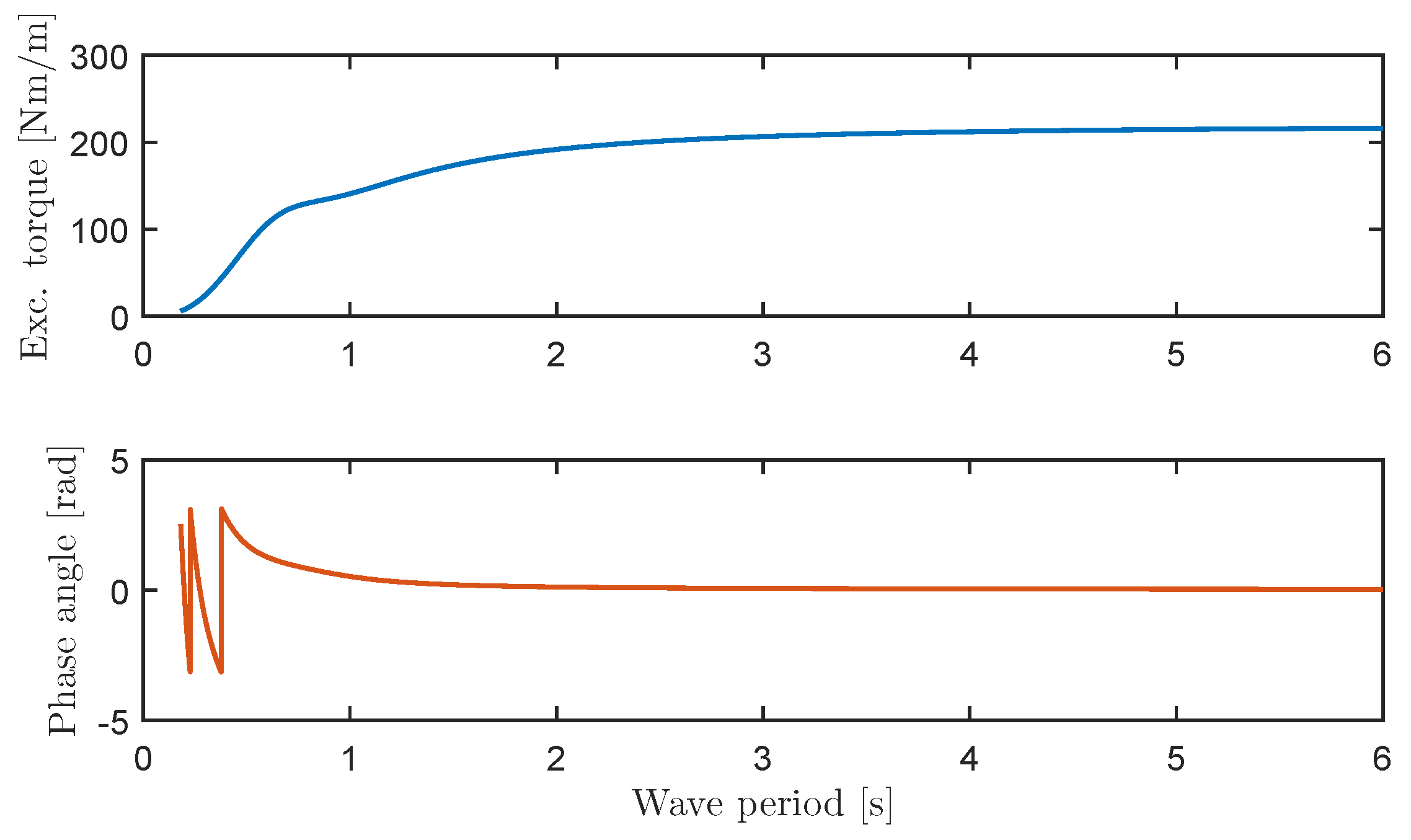
3.2. Hydrodynamic Parameters

For the setup at hand, it is practical to express the hydrodynamic parameters in terms of rotation about the pivot A (cf. Figure 2). This can be achieved by defining the geometric model with the constraint that it has to move about that axis. The hydrodynamic parameters from the boundary element solver will then be given directly as a function of rotation angle. This approach was used here. The excitation torque is shown in Figure 4.

Figure 4. Hydrodynamic excitation torque on the experimental model.

3.3. Optimal Load Resistance for Unconstrained Oscillation

According to linear theory, when disregarding losses, the optimal load resistance $R_{\mathrm{opt}}$ for a one-degree-of-freedom system undergoing harmonic oscillation may be found as [17]

$$R_{\mathrm{opt}}\left(\omega \right)=\sqrt{R_r{\left(\omega \right)}^2+X{\left(\omega \right)}^2}X\left(\omega \right)=\omega J_A\left(\omega \right)-S_{\phi }/\omega$$

(14)

where $R_r\left(\omega \right)$ and $X\left(\omega \right)$ are the radiation resistance and the reactance of the system, respectively, and $J_A\left(\omega \right)=J_{\mathrm{buoy}}+J_{\mathrm{ballast}}+J_{\mathrm{lever}}+J_r\left(\omega \right)$ is the moment of inertia about the pivot A including added inertia as discussed before, but here including the frequency-dependent part. The resonance of the system is defined by the reactance X being zero, and it can be tuned by changing the mass and/or stiffness of the system. Assuming that the mass is kept constant, but the stiffness is modified to achieve resonance at a frequency of $f_0={\omega }_0/\left(2\pi \right)=1/T_0=1/1.5\mathrm{s}=0.67$ Hz the required stiffness S becomes

$$X=0\to S={\omega }_0^2{J}_A\left({\omega }_0\right).$$

(15)

Still assuming absence of losses, the optimal energy absorption in a regular wave of period $T_0$ is then obtained by damping: $R_{\mathrm{opt}}=R_r\left({\omega }_0\right)$.

The estimated impedance terms for the WaveStar laboratory model in original and tuned configurations (stiffness adjusted to obtain resonance at $T_0=1.5$ s) are shown in Figure 5, and the corresponding theoretical (unconstrained) power response curves are found in Figure 6.

Figure 5. Reactance (dashed) and optimal load resistance (solid) estimated for the system under the assumption of no losses for both a system with original configuration (blue) and a system with stiffness tuned to give resonance at $T_0=1.5$ s (green). The large-mass system has been assumed, cf. Table 2.

Figure 6. Power response for the system with original configuration (blue) and with stiffness tuned to give resonance at $T_0=1.5$ s (green). The power response is drawn for a wave amplitude of 12.5 mm assuming no amplitude constraints. The mass alternatives small and large refer to Table 2.

3.4. Optimal Load Resistance for Constrained Oscillation

When the oscillation amplitude is constrained, the load resistance needs to be adjusted as a function of wave height and period in order for the motion response not to violate the angular excursion constraint $\phi \le {\phi }_{\max }$. For sinusoidal motion, this may be rewritten as a constraint on the angular velocity $u=\dot{\phi }$, expressed as $|\widehat{u}| \le u_{\max }=\omega {\phi }_{\max }$.

Expressing the variables in terms of complex amplitudes ${\widehat{\tau }}_e$ for the excitation torque and $\widehat{u}$ for the angular velocity, the oscillation amplitude can be written as a function of the absolute value of impedance $|Z|=|R+iX|=\sqrt{R^2+X^2}$ through

$$|\widehat{u}| = |{\widehat{\tau }}_e|/|Z| = |{\widehat{\tau }}_e|/\sqrt{R^2+X^2}$$

(16)

where $R=R_r+R_m$ is the sum of radiation resistance and machinery damping $R_m$. Constraining the angular velocity to $|\widehat{u}| \le u_{\max }$, a machinery damping $R_m=R_c$ that will fulfil the requirement is to be found. Inserting now $|\widehat{u}| = u_{\max }$ and $R=R_r+R_c$ into Equation (16) gives

$${(R_r+R_c)}^2={|{\widehat{\tau }}_e|}^2/u_{\max }^2-X^2$$

(17)

where the solution looked for is

$$R_c=\sqrt{|{\widehat{\tau }}_e{|}^2/u_{\max }^2-X^2}-R_r,R_m=\max (R_c,R_{\mathrm{opt}}).$$

(18)

The right-hand expression ensures that the optimal unconstrained damping is used when the maximum amplitude has not been reached.

In case of perfect phase control, $X=0$, and the solution reduces to

$$R_c=|{\widehat{\tau }}_e|/u_{\max }-R_r{R}_m=\max (R_c,R_r).$$

(19)

4. Experimental Testing Conditions

This section presents the model variations tested during the experimental campaign and the regular and irregular wave conditions tested. An overview of the runs carried out during the experimental campaign can be found in the appendix.

4.1. Model Variations

Several configurations have been tested during the experimental campaign and are listed in Table 2.

In order to assess the effect of the WaveSpring, the configuration with (Setups 3, 4, and 5) and without the WaveSpring (Setups 1 and 2) have been tested. The mass of the buoy is another parameter that has been varied in the current work. The system is referred to as "unballasted" for the lower mass and "ballasted" for the higher mass. For both configurations, the system was adjusted to ensure the buoy was in equilibrium position in still water. In Setup 3, the shortest spring length is slightly smaller than that for Setups 4 and 5, leading to a higher negative stiffness effect on the system.

The machinery damping $R_m$ provided by the PTO was varied in four levels for regular wave runs, and chosen as a constant for the irregular wave runs (cf. Appendix A).

4.2. Wave Conditions

All sea states were run in the basin without model installed in order to establish the undisturbed wave field and measure the resulting wave parameters in each case. Table 3 and Table 4 describe the realized regular and irregular waves, respectively, used in the experiment. A resistive wave probe placed next to the buoy model (cf. Figure 3) was used for the given analysis and for the analysis of the motion response, Section 5. When calculating amplitude responses, the wave measured in open tank (without the model) was used as measurement of the incident wave.

Table 3. Description of the realized regular wave sea states in terms of wave period and wave height as measured in the basin without the model.

Name	Wave Period	Wave Height
	$\mathit{T}\left[\mathbf{s}\right]$	Target ${\mathit{H}}_{\mathbf{tar}}\left[\mathbf{m}\right]$	Measured ${\mathit{H}}_{\mathbf{mes}}\left[\mathbf{m}\right]$	Reference ${\mathit{H}}_{\mathbf{ref}}\left[\mathbf{m}\right]$
Rf1	0.7	0.0300	0.0293	0.0250
Rf2	0.9	0.0300	0.0270	0.0250
Rf3	1.1	0.0300	0.0250	0.0250
Rf4	1.3	0.0300	0.0250	0.0250
Rf5	1.5	0.0300	0.0230	0.0250
Rf6	1.7	0.0300	0.0236	0.0250
Rf7	1.9	0.0300	0.0236	0.0250
Rf8	2.1	0.0300	0.0225	0.0250

Table 4. Description of the realized irregular wave sea states in terms of wave height ($H_{m0}$) and wave periods ($T_{0,2}$,$T_{-1,0}$), as measured in the basin without the model.

Seastate	${\mathit{H}}_{\mathit{m}0}\left[\mathbf{m}\right]$	${\mathit{T}}_{0,2}\left[\mathbf{s}\right]$	${\mathit{T}}_{-1,0}\left[\mathbf{s}\right]$
S1	0.0193	0.778	0.869
S2	0.0556	1.029	1.205
S3	0.0895	1.334	1.596

For the irregular waves, a frequency analysis was performed to obtain the wave height ($H_{m0}$), the average wave period ($T_{0,2}$) and the energy period ($T_{-1,0}$).

Some considerations regarding wave reflection in the wave basin have been done. When waves arrive at the model, they induce body motion and wave scattering. Scattered and body-generated waves will return to the model after reflection at the side walls, sloping beach, and wave maker paddles. Of these reflecting surfaces, the model is closest to the bottom end of the sloped beach, which starts 3550 mm from the center axis of the buoy model. However, as this is a rubble mound beach extending all the way down to the bottom, we consider that the part of it closest to the model does not have a significant effect. The beach mean water line is at 8850 mm from the model. It is assumed that reflections from the walls at distance $d_{\mathrm{wall}}=4250$ mm from the model will be the first to influence the model response.

The time $T_r$ for the waves to travel from the model to the side wall and back may be found as

$$T_r=2\frac{d_{\mathrm{wall}}}{v_g}$$

(20)

where $v_g$ is the group velocity of the waves. For regular wave runs, this corresponds to a time in the range $[4.6,15.5]$ s, leaving only two full undisturbed wave cycles for the regular waves of the longest period. Only the undisturbed wave cycles were used in the analysis for regular waves. The irregular wave sea states were synthesized with about 110 wave cycles, and the full recorded time series was used in the analysis.

5. Results and Discussion

This section presents the results of the experimental campaign together with a discussion based on those results. It includes an uncertainty analysis, hydrostatic stiffness and friction measurements, characterization of the WaveSpring torque, capability of the PTO system, and experimental results for both regular and irregular wave conditions.

5.1. Uncertainty

An analysis of the uncertainty related to the instrumentation used during the experimental campaign has been performed. The analysis was done on the velocity measurement before and after the Kalman filter and on the torque measurement. The results are tabulated in Table 5. Forty test runs on Setup 3 were used, where the frequency of the signal (i.e., of the wave) was filtered out and the spikes caused by static friction at zero velocity were removed.

Table 5. Uncertainty on torque and velocity measurements.

Measurement	Unit	Uncertainty
$\tau$	Nm	0.05
v	rad/s	0.03
$v_{Kalman}$	rad/s	0.02

Note that the laser-based sensor provides only the offset position for the signals from the accelerometer. The power calculations were performed using the velocity signal after the Kalman filter and the torque measurement.

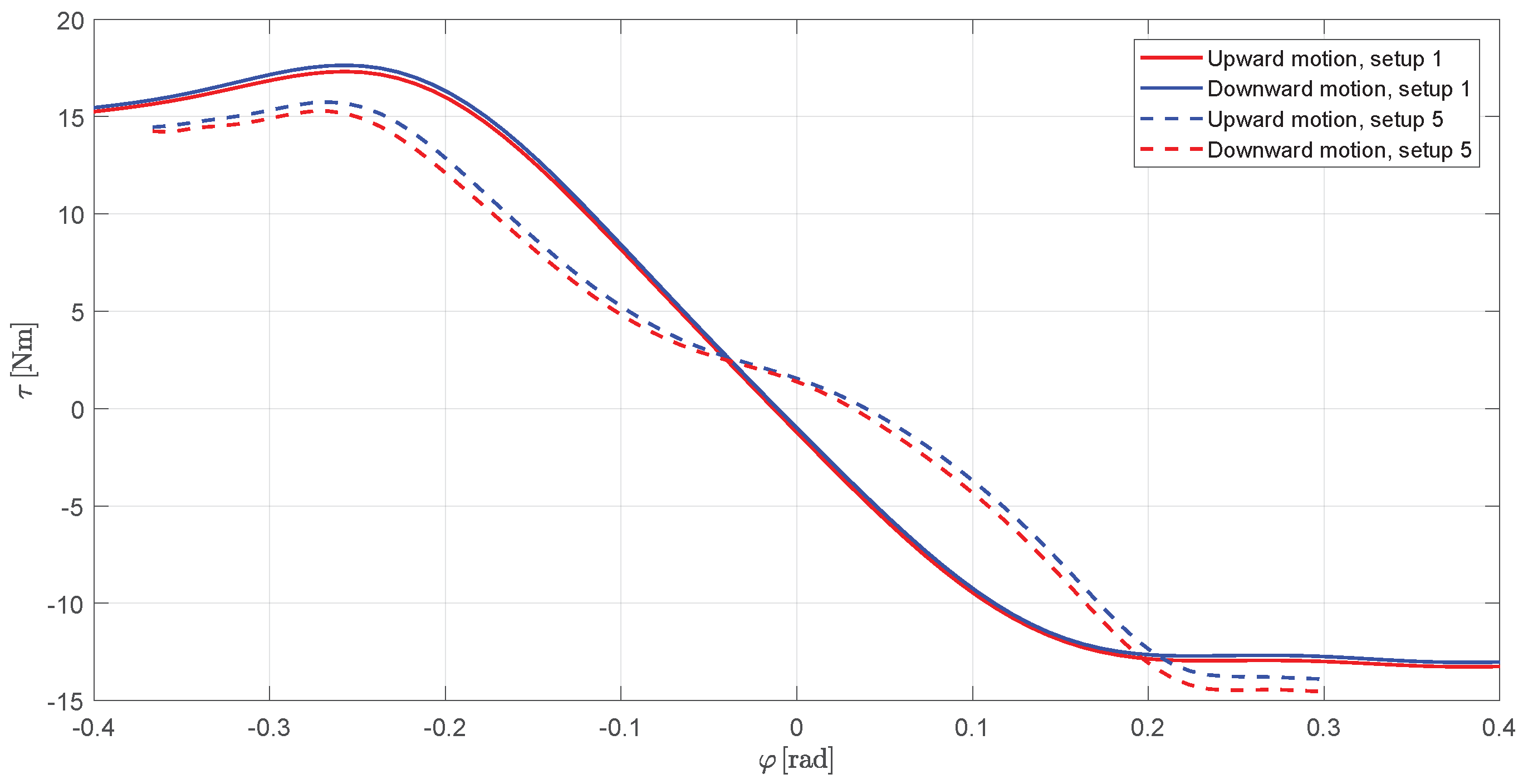
5.2. Hydrostatic Stiffness

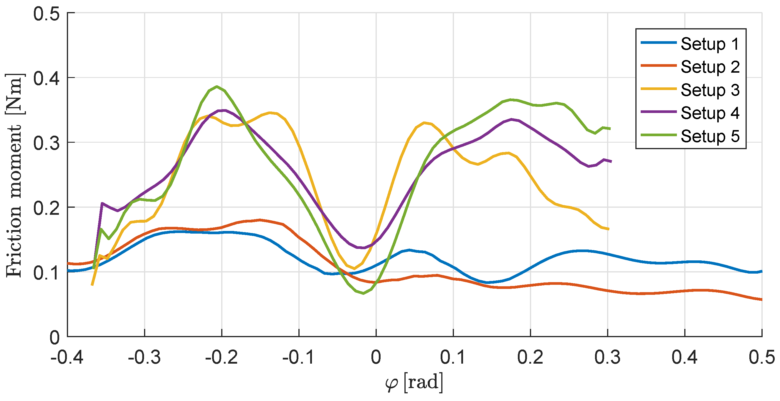
Slow forced oscillations tests were performed in order to quantify the hydrostatic stiffness of the different system configurations. The period of the forced sinusoidal motion was 100 s. Figure 7 shows the measured reaction torque about the rotation axis as a function of rotation angle in configurations with ballast mass (i.e., Setups 1 and 5). It can easily be observed that the WaveSpring mechanism reduces the stiffness, determined from the slope of the curve, in the midpoint range. The estimated stiffness coefficient in this range is shown in Table 6 for all system configurations. Peak values and the value estimated for nominal zero angle are also tabulated.

Figure 7. Measured reaction torque about rotation axis for slow forced oscillation in calm water with Setups 1 and 5.

Table 6. Hydrostatic stiffness estimated for the different system configurations from slow forced oscillations in calm water. The values referred to as mean are computed as the average over the rotation angle interval [−0.05, 0.05] rad. The resonance period estimated in the three last columns refer to the corresponding stiffness values in the three first columns. Note that the peak values refer to a maximum value for setups without WaveSpring (Setups 1 and 2), and a minimum value for setups with WaveSpring (Setups 3–5), cf. Figure 7.

Configuration	Stiffness [Nm/rad]			Resonance Period [s]
	${}^{\mathbf{1}}$Mean	${}^{\mathbf{2}}$Peak	${}^{\mathbf{3}}$at$\mathbf{\phi }=\mathbf{0}$	${}^{\mathbf{1}}{\mathit{T}}_{\mathbf{0}}$	${}^{\mathbf{2}}{\mathit{T}}_{\mathbf{0}}$	${}^{\mathbf{3}}{\mathit{T}}_{\mathbf{0}}$
Setup 1	88.5	95.6	91.5	0.807	0.770	0.791
Setup 2	85.4	93.8	89.3	0.637	0.599	0.619
Setup 3	33.4	9.13	21.4	1.15	2.31	1.47
Setup 4	42.3	23.2	29.0	1.00	1.41	1.25
Setup 5	45.2	26.3	32.8	1.18	1.58	1.40

Table 6 also shows that the ballast tends to slightly increase the stiffness, as should be expected due to the change in angular component of gravity. The difference in mean stiffness between Setups 3 and 4 due to different compression of the coil spring is about 9 Nm/rad.

It is interesting to compare the measured change in stiffness coefficients to the effective stiffness coefficient estimated by Equation (5). Inserting numbers for Setup 4 from Table 1 and Table 2 gives an effective WaveSpring rotational stiffness of −60.4 Nm/rad. This corresponds well to the change in rotational stiffness values observed between Setups 2 and 4, which are −70.6 Nm/rad (peak value) and −60.3 Nm/rad (nominal zero angle value).

5.3. Friction

The slow forced oscillations tests were also used to derive an estimate of the static friction of the system with and without the WaveSpring mechanism, as explained in Section 3 and illustrated in Figure 8.

Figure 8. Estimated static friction torque for the different system configurations.

It is assumed that the friction in the tests presented here is dominated by the static friction part, and the friction in the wave response tests is estimated directly from the friction curves shown in Figure 8 by choosing a constant after visual inspection.

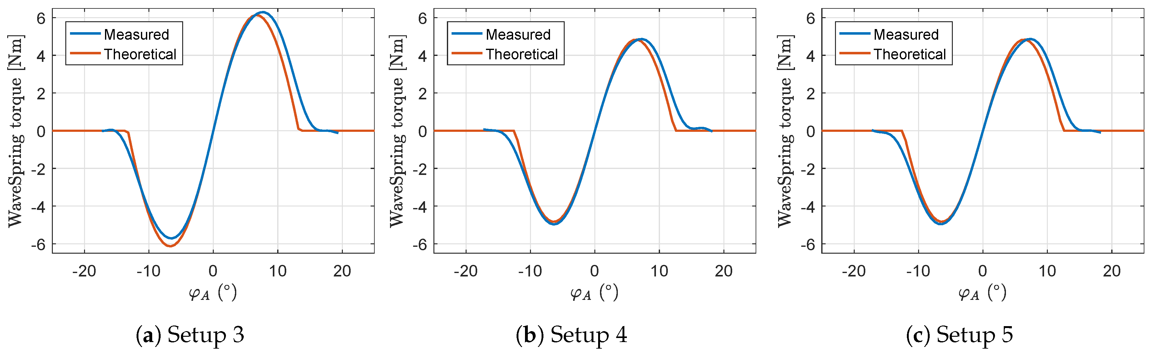
5.4. WaveSpring Torque

An estimate for the net spring torque from the WaveSpring mechanism was found by comparing the slow-oscillation torque curves with and without the coil spring component mounted, i.e., Setups 3 and 4 were compared with Setup 2 (unballasted), and Setup 5 was compared with Setup 1 (ballasted). Figure 9 shows a comparison of measured and computed torque curves. The correspondence between the theoretical (Equation (3)) and measured curves has been improved by adjusting the coil spring stiffness from the tabulated value $k_{\mathrm{coil}}=1.32$ kN/m (cf. Table 1) to $k_{\mathrm{coil}}^{\prime }=1.50$ kN/m.

Figure 9. Theoretical and measured values for ${\tau }_{\mathrm{WS}}$ as a function of the rotation about pivot A for the different setups equipped with the WaveSpring mechanism.

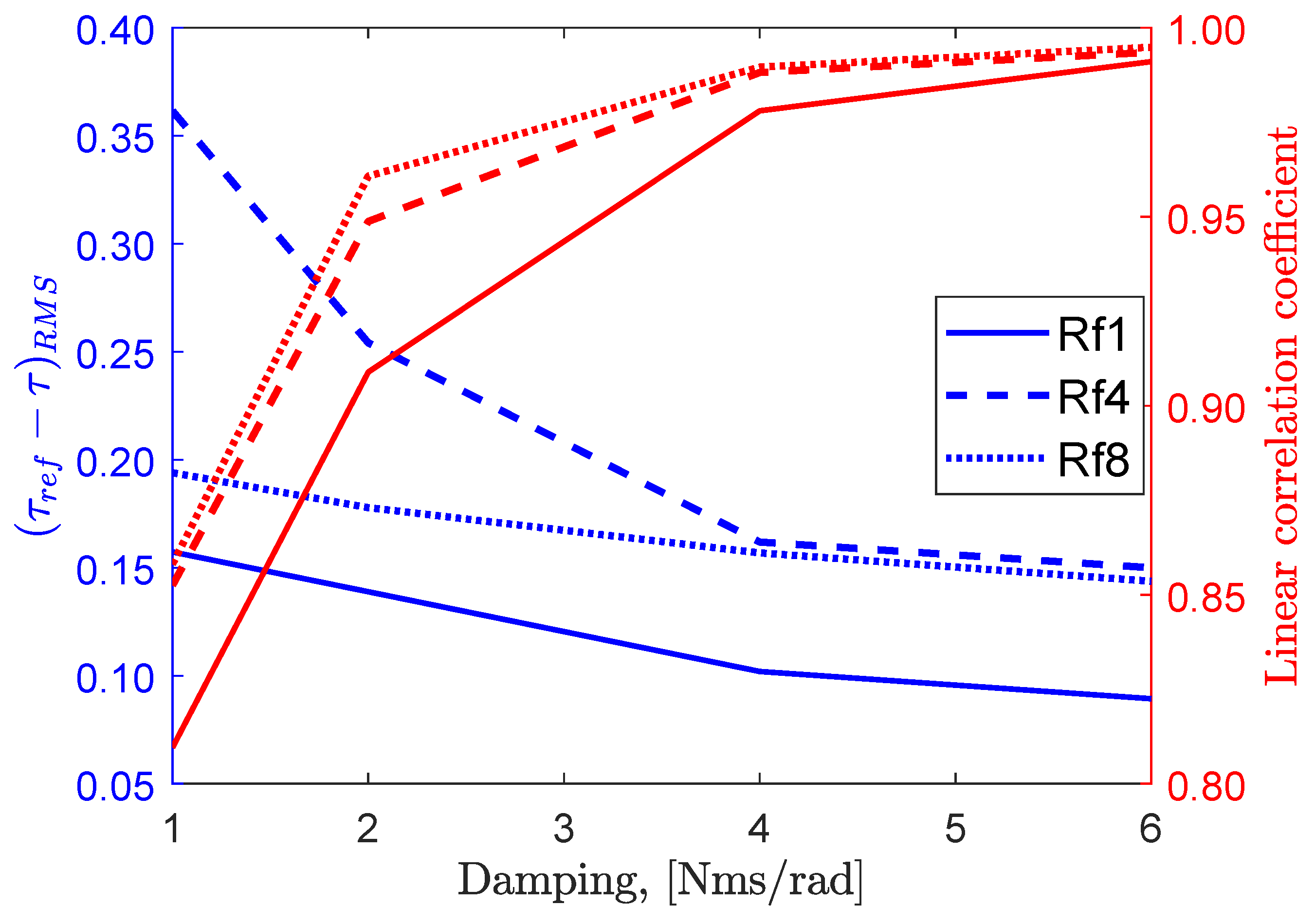
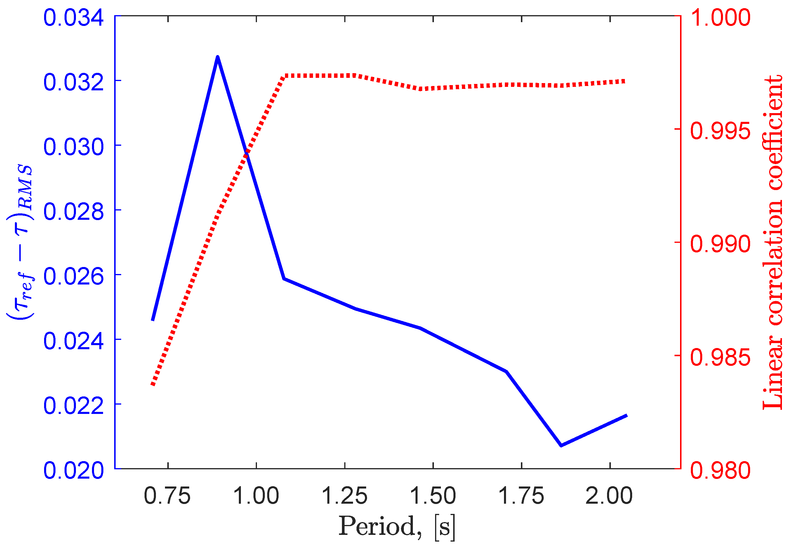
5.5. Actuator Reference Following

The PTO system used in the experimental setup described in Section 2 corresponds to a subsystem with its own frequency response. As the configuration of the controller is limited, this subsystem is not perfectly tuned for the buoy characteristic and this translates into a frequency and machinery damping dependency of the quality of the reference following.

Figure 10 shows the frequency dependency of the actuator’s reference following behavior in terms of the root-mean-square (RMS) of the difference between the reference (${\tau }_{ref}$) and the measured torque ($\tau$) defined as

$${({\tau }_{ref}-\tau )}_{RMS}=\sqrt{\frac{1}{N}\sum _{n=1}^N{|{\tau }_{ref,n}-{\tau }_n|}^2}$$

(21)

and in terms of the linear correlation coefficient between the reference torque and the measured torque:

$$\rho ({\tau }_{ref},\tau )=\frac{\mathrm{cov}({\tau }_{ref},\tau )}{{\sigma }_{{\tau }_{ref}}{\sigma }_{\tau }}$$

(22)

where $\mathrm{cov}$ stands for the covariance of ${\tau }_{ref}$ and $\tau$, and $\sigma$ is the standard deviation. All regular wave conditions were used to compute this frequency dependency. In this case, the machinery damping was set to the optimal value determined from linear theory. As no friction compensation is included in the configuration of the controller, spikes caused by friction at zero velocity were filtered out of the torque measurement. The controller is performing better for higher wave periods, i.e. from Rf3 to Rf8. The linear coefficient drops for wave periods lower than 1.1 s but still remains relatively high for optimal damping condition.

Figure 10. Frequency dependency of the actuator reference following capability in terms of the root-mean-square (RMS) of $({\tau }_{ref}-\tau )$ and in terms of linear correlation coefficient between ${\tau }_{ref}$ and $\tau$, for Setup 3. Note that the wave period has been chosen as the x-axis to better relate to the different regular waves used during the experimental campaign.

Figure 11 presents the same performance factors as previously discussed as a function of machinery damping for three different regular wave conditions: Rf1, Rf4, and Rf8. The dependency on the machinery damping of the controller’s ability to follow the reference is easily seen. For low machinery damping the performances drop drastically, and more so for lower wave period (Rf1). It is important to note that the power analysis performed and presented later in this work are for optimal conditions where the system performs nicely, as depicted in Figure 10.

Figure 11. Machinery damping dependency of the actuator reference following capability in terms of the RMS of $({\tau }_{ref}-\tau )$ and in terms of linear correlation coefficient between ${\tau }_{ref}$ and $\tau$, for Setup 3.

5.6. Regular Wave Results

Motion response of the different system configurations described in Section 4.1 were performed in regular waves in order to demonstrate the working principle of the WaveSpring mechanism and validate the mathematical model. It is important to note that the machinery damping was only optimized for one configuration, namely Setup 3. For the other setups, the optimal machinery damping obtained from linear theory was used. With the WaveSpring mechanism, the damping was sometimes set to a higher value to avoid excessive motions and full submergence or water exit. The values used are listed in Appendix A.

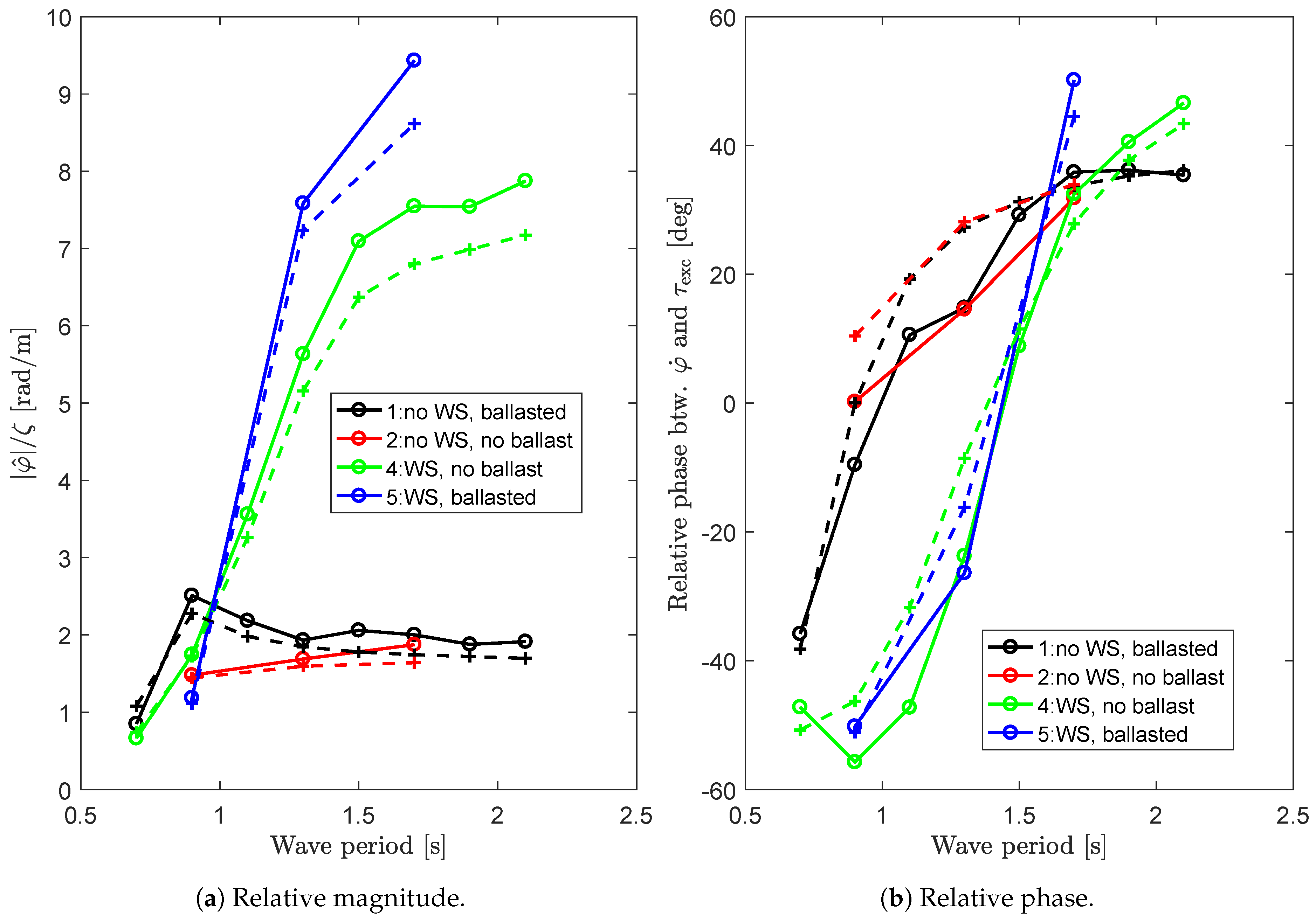
5.6.1. Motion Response in Regular Waves

The motion response is analyzed in terms of amplitude and phase responses for input waves of wave height 30 mm (setpoint) and varying wave period. These have been derived by taking the discrete Fourier transform of the steady-state part of the response time series, which corresponds to the time interval before wave reflections reach the model (cf. Section 4.2). Before transformation the time series was cut to an integer number of cycles to avoid spectral leakage. The amplitude response is then computed as the magnitude of the fundamental harmonic component of the spectrum, which corresponds to the wave frequency.

Figure 12 shows amplitude responses for angular excursion for the four configurations Setups 1, 2, 4, and 5. The WaveSpring mechanism strongly amplifies the motion in the wave period range from about 1 s and above. For lower wave periods, the response is stronger for configurations without WaveSpring, as these have their resonance period in the range 0.8–1.0 s.

Figure 12. (a) Amplitude response and (b) relative angle between angular velocity and excitation torque. The phase is given as relative angle between angular velocity and excitation torque. Circle markers show the laboratory results, while crosses show the model results. Numbers 1, 2, 4, and 5 in the legend correspond to Setups 1, 2, 4, and 5, respectively.

The velocity phase response is also shown in Figure 12. Instead of the wave elevation phase, the phase of the excitation torque is used as reference, as this more clearly shows the resonance and bandwidth properties of the system. It should be noted that, in the case of runs without WaveSpring (Setups 1 and 2), the machinery damping was set according to the theoretically optimal value (in the range 3.5 to 26 Nms/rad in non-equal steps, cf. Figure 6 and Appendix A). This improves the phase response for these runs. Correspondingly, for the runs with the WaveSpring mechanism, the machinery damping was varied in the range 1.0–6.9 Nms/rad in non-equal steps. The phase of the excitation torque was estimated numerically from the linear theory. The results show how the WaveSpring mechanism shifts the resonance period, identified as zero phase difference, from around 0.8 s to about 1.4–1.5 s. Despite the few measurement points, it is also worth noticing how the phase responses of Setups 4 and 5 differ. The larger inertia of Setup 5 makes its phase response steeper around resonance than for Setup 4. This means that Setup 4 has a larger bandwidth, which is a beneficial property when operating in irregular waves.

An example of the buoy motion in regular wave Rf5 is shown in Figure 13. This demonstrates how the WaveSpring mechanism in Setup 4 makes the buoy oscillate with larger amplitude than the incident wave, and how the velocity is almost in phase with the estimated excitation torque for this wave, which has a period close to the tuned resonance. For Setup 1, the large damping also results in a fairly good phase response, but this comes at the expense of much lower oscillation amplitude.

Figure 13. Buoy motion for regular wave Rf5, comparing the responses of Setups 1 and 4. In the left diagram, the buoy travel is expressed as excursion along the circular path through point B with the center at pivot A, cf. Figure 2. All signals have their mean values extracted.

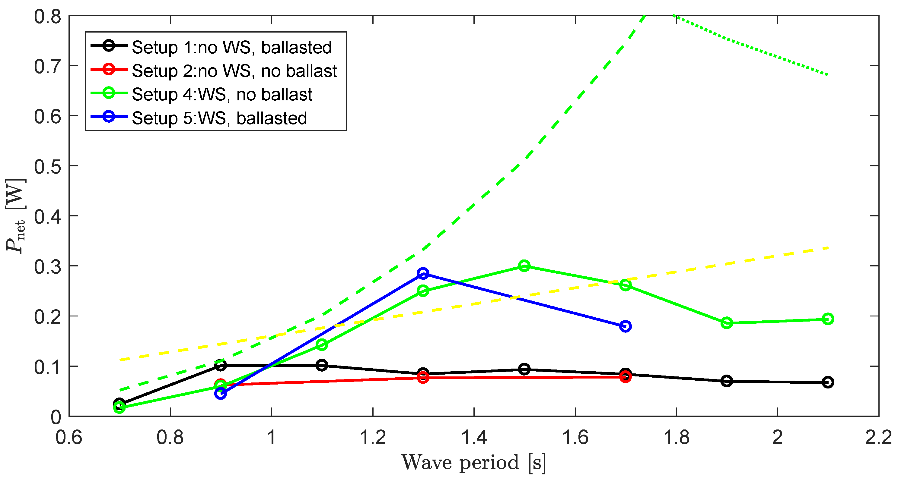
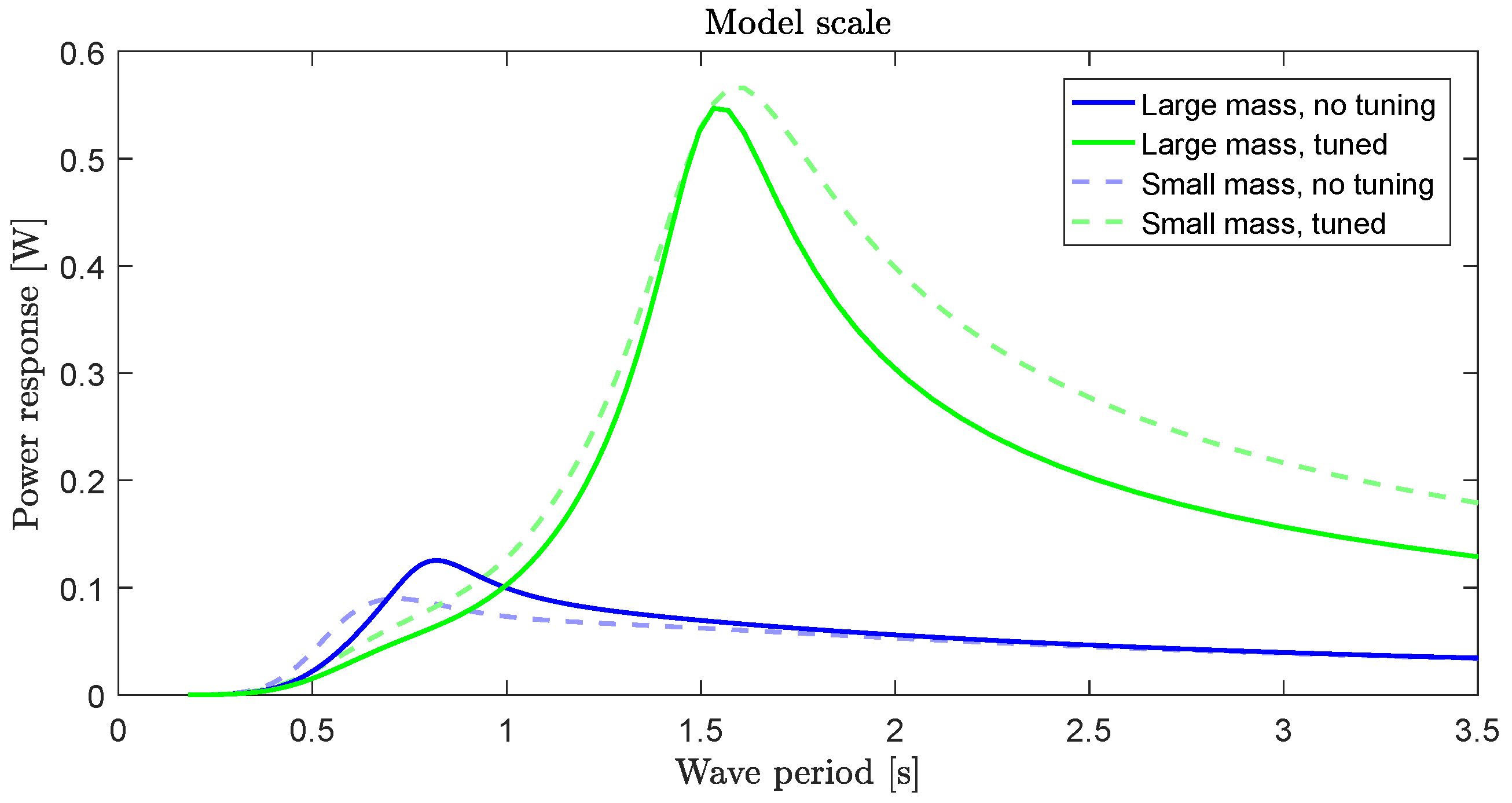
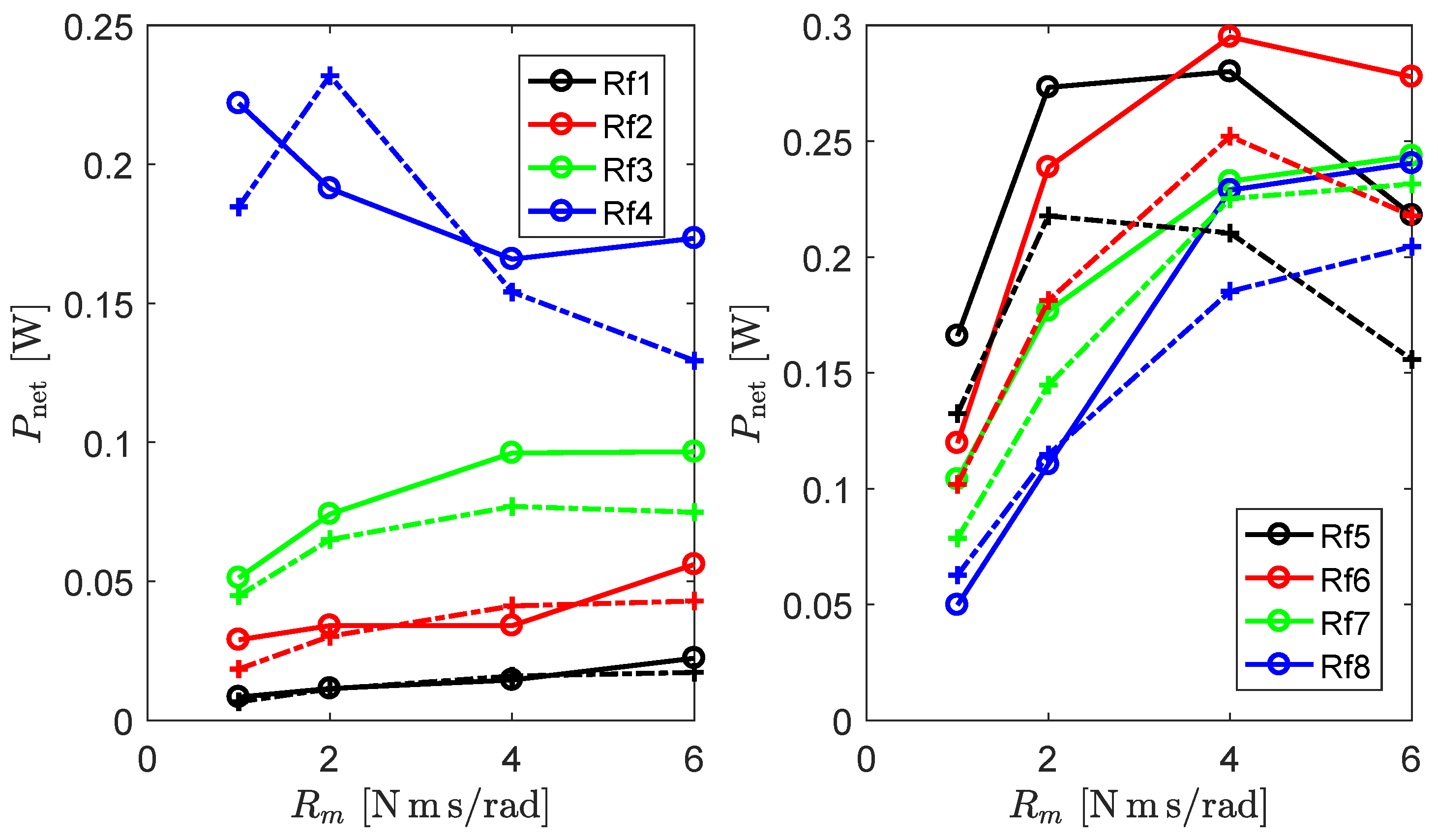
5.6.2. Power Absorption in Regular Waves

In order to calculate the power absorption, the following definitions are defined and illustrated in Figure 14:

Figure 14. Assumed energy flow and associated definitions for the laboratory model.

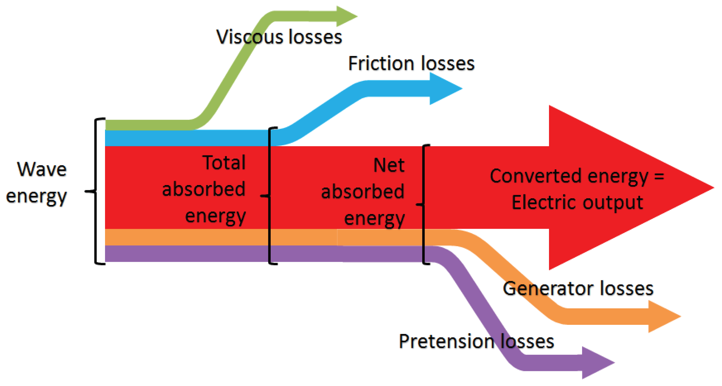
• Wave energy: Total energy taken from the wave field.
• Total absorbed energy: Total energy absorbed into the mechanical system from the water.
• Net absorbed energy: Absorbed energy as measured on the load cell between the actuator and the rotating arm that holds the buoy. Losses between total absorbed energy and net absorbed energy include friction losses in the shaft bearings and the WaveSpring mechanism.
• Converted energy: Derived quantity based on subtracting assumed losses between net absorbed energy and electrical energy output, notably losses in the electric generator and the pretension system. The generator losses are estimated based on the conversion efficiency for a typical electric generator. When the system works with pretension, some energy will be lost in the pretension mechanism. This loss is computed as a loss fraction $f_{pre}$ on the pretension torque, $P_{loss}=f_{pre}{\tau }_{pre}{v}^2/|v|$.

The average converted power as measured by the load cell at the lever is plotted in Figure 15. The data points have been scaled by the factor ${(H_{\mathrm{ref}}/H_{\mathrm{mes}})}^2$ for the incident wave. The reference wave height has been set to 0.025 m, cf. Table 3. The figure shows how the ballasted system performs somewhat better than the unballasted system when there is no WaveSpring mechanism, as should be expected due to the larger resonance period of the ballasted system. Also shown in the figure are the theoretical limit for unconstrained heave motion of an axisymmetric buoy, as well as a yellow line corresponding to the amount of power passing over a width equal to the buoy diameter. With the WaveSpring mechanism, there is a strong increase in absorbed power for waves with a period larger than 1.0 s. It may be observed that, with the WaveSpring mechanism, the system is indeed able to obtain a point absorber effect that makes the absorption width larger than the physical width of the buoy. The three points found above the yellow line represent relative capture width of between 1.2 and 1.4. In addition to the tuned phase response, the system is also taking benefit from a combined surge and heave motion of the buoy. Further modeling and analysis may show the relative contribution from these two oscillation modes.

Figure 15. Average net absorbed power. Also shown are the upper theoretical limits for an axisymmetric heaving body (green, dashed) and Budal’s upper bound (green, dotted). The yellow dashed line shows the amount of power passing over a width equal to the buoy diameter.

Some of the power absorbed from the wave is lost in friction, in particular in friction as measured for the WaveSpring mechanism (see Section 5.3). If the power lost in friction is included to compute the total absorbed energy, the measured relative absorption width reaches up to about 1.6.

Figure 15 may also be compared to Figure 6 that considers theoretical results for unconstrained motion. Together with friction and viscous loss, the reduction of the WaveSpring torque outside the $\phi \in [-{10}^{\circ },{10}^{\circ }]$ range is found to be the main reason why the curves for measured tuned response peak earlier than the theoretical curves. Above about 1.3 s wave period, oscillation amplitudes beyond ${10}^{\circ }$ are needed to approach the theoretical limit.

It is important to mention that the PTO efficiency, which would typically reduce all power estimates by 10–40%, have been disregarded in all results presented, both with and without the WaveSpring.

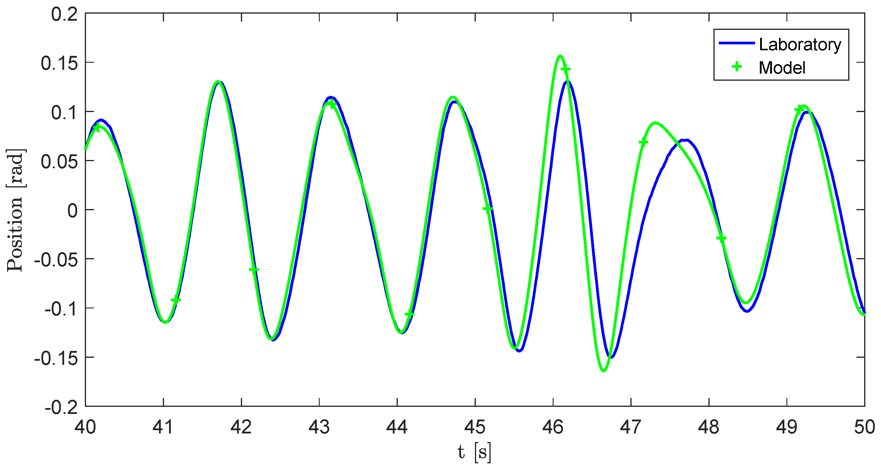
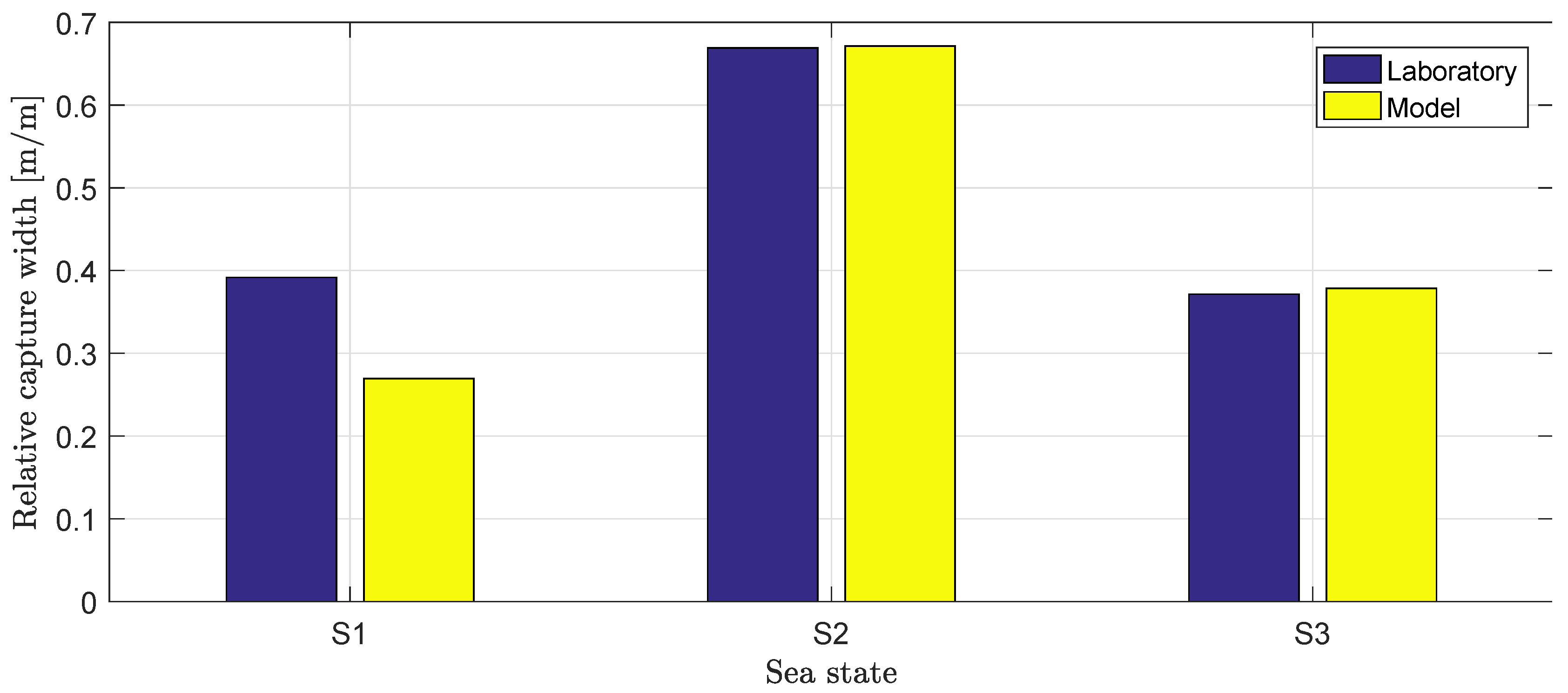
5.6.3. Mathematical Model Validation

The mathematical model described in Section 3 has been used to simulate the response measured during the experimental campaign. The analytical expression for the WaveSpring force derived in Equation (3) was used in the model. The amplitude and phase responses obtained by the model were included in Figure 12, along with the experimental results for Setups 1, 2, 4, and 5.

The simple model developed and presented in Section 3 is able to capture the general behaviour of the systems without and with the WaveSpring even though the latest introduces non-linearities in the system. The model captured better the amplitude response in short waves than the amplitude response in intermediate and long waves. The phase response diagrams clearly show how the model has significant deviations from measurements in the mid-range of wave periods. This is the case for all experimental setups.

The difference in phase between the model and experimental results could be an effect of not taking into account the difference in instantaneous inertia. The buoy is moving in and out of the water, and at the same time it varies in the relative contribution from heave and surge. In principle, the equation of motion should then include the change-in-mass term $dm/dt$. The models are all linearized in angular motion, with mass-properties depending only on frequency, and does not take these effects into account. The rigid body mass was estimated from weighing all the different parts of the system; it is not expected to be far off, although there is obviously limited accuracy. The model may not represent the stiction accurately, but the effect should be less dependent on frequency. The phase lag could not be reproduced in the model by increasing the static friction in the setups. Finally, the phase response for the experimental runs is based on estimating the phase of the excitation force using theoretical excitation force coefficients. The correctness of this phase has not been validated with measurement. Further experiments or computational fluid dynamics studies would probably be needed to further investigate the observed deviations.

A variation of machinery damping was performed for Setup 3. As known from theory, summarized in Section 3.4, for a linear system, each wave period will have one value for the machinery damping that maximizes the absorbed power. Based on linear theory with friction disregarded, the optimum value for the machinery damping is predicted to lie in the interval from about 1 to 6 Nms/rad. The machinery damping was varied accordingly in four levels: 1, 2, 4, and 6 Nms/rad. Measured values are shown in Figure 16. Also shown in Figure 16 is how the dependency on machinery damping is well captured by the simulation model. In short waves, the fit is difficult to assess as the experimental data is strongly influenced by the less accurate reference-following of the actuator, cf. Section 5.5. There is a difference in sea states Rf1 and Rf2 around applied damping of 4 Nms/rad which has not been captured by the model. This might be an effect of less accurate reference-tracking or uncertainties in measurements and processing, but overall the dependency on machinery damping is clearly captured in the numerical model.

Figure 16. Simulation results (crosses) and experimental measurements (circles) for the net absorbed power for the difference regular wave conditions (Rf1 to Rf8).

5.7. Irregular Wave Results

Figure 17 shows an example of time series for simulation results compared to experimental measurements in irregular waves. As for regular waves, the dynamics of the system are well captured by the model in irregular wave conditions.

Figure 17. Angular displacement time series comparison for Setup 5 and wave conditions S2 where the blue solid line corresponds to laboratory measurements, while the green solid line with crosses corresponds to the simulation results.

Figure 18 shows the estimated power response for sea states S1, S2, and S3 and Setup 5, both in terms of total absorbed power and net absorbed power, based on experimental results and simulation. The model gives better predictions for sea states S2 and S3 than for S1. This can most likely be attributed to the less accurate reference-tracking in the short wave period range.

Figure 18. Average absorption width in irregular wave sea states, where experimental data is compared to results from the mathematical model for Setup 5. Blue: Experimentally determined relative capture width. Yellow: Capture width determined from simulation results.

6. Conclusions

The dynamics of a pitching wave energy converter were studied both in laboratory tests and numerical simulations. The laboratory model was equipped with a new spring mechanism that improves the response properties of the system. A simple mathematical model was developed and has been shown to capture the dominating dynamic effects. The laboratory model of a negative spring mechanism clearly demonstrated the potential of such solutions in making wave energy converters more efficient. Practical implementation in full scale will show the real increase in performance that may be achieved.

References

- Hals, J.; Bjarte-Larsson, T.; Falnes, J. Optimum reactive control and control by latching of a wave-absorbing semisubmerged heaving sphere. In Proceedings of the International Conference on Offshore Mechanics and Arctic Engineering, Oslo, Norway, 23–28 June 2002. [Google Scholar]
- Cretel, J.; Lightbody, G.; Thomas, G.; Lewis, A. Maximisation of Energy Capture by a Wave-Energy Point Absorber using Model Predictive Control. Available online: http://folk.ntnu.no/skoge/prost/proceedings/ifac11-proceedings/data/html/papers/3255.pdf (accessed on 10 July 2018).
- Ringwood, J.; Bacelli, G.; Francesco, F. Energy-Maximizing Control of Wave-Energy Converters: The Development of Control System Technology to Optimize Their Operation. IEEE Control Syst. Mag. 2014, 6, 30–55. [Google Scholar] [CrossRef]
- Van Niekerk, J.L.; de Fallaux Retief, G. Wave energy convertor, 2015. U.S. Patent 1,313,2206, 10 December 2008. [Google Scholar]
- Zhang, X.; Yang, J.; Xiao, L. Numerical study of an oscillating wave energy converter with nonlinear snap-through Power-Take-Off systems in regular waves. J. Ocean Wind Energy 2014, 10, 225–230. [Google Scholar]
- Todalshaug, J.H.; Ásgeirsson, G.S.; Hjálmarsson, E.; Maillet, J.; Möller, P.; Pires, P.; Guérinel, M.; Lopes, M. Tank testing of an inherently phase-controlled wave energy converter. Int. J. Mar. Energy 2016, 15, 68–84. [Google Scholar] [CrossRef]
- Zhang, X.; Yang, J. Power capture performance of an oscillating-body WEC with nonlinear snap through PTO systems in irregular waves. Appl. Ocean Res. 2015, 52, 261–273. [Google Scholar] [CrossRef]
- Zurkinden, A.; Ferri, F.; Beatty, S.; Kofoed, J.; Kramer, M. Non-linear numerical modeling and experimental testing of a point absorber wave energy converter. Ocean Eng. 2014, 78, 11–21. [Google Scholar] [CrossRef]
- Zurkinden, A.S.; Kramer, M.M.; Ferri, F.; Kofoed, J.P. Numerical Modeling and Experimental Testing of a Wave Energy Converter: Deliverable D4.2; Department of Civil Engineering, Aalborg University: Aalborg, Denmark, 2013. [Google Scholar]
- Kramer, M.; Marquis, L.; Frigaard, P. Performance Evaluation of the Wavestar Prototype. In Proceedings of the 9th European Wave and Tidal Energy Conference, Southampton, UK, 5–9 September 2011. [Google Scholar]
- Wahl, A.M. Mechanical Springs, 2nd ed.; Penton Publishing Company: Cleveland, OH, USA, 1963. [Google Scholar]
- Beatty, S.; Ferri, F.; Bocking, B.; Kofoed, J.P.; Buckham, B. Power Take-Off Simulation for Scale Model Testing of Wave Energy Converters. Energies 2017, 10, 973. [Google Scholar] [CrossRef]
- WAMIT User Manual. 2006. Available online: http://www.wamit.com (accessed on 10 July 2018).
- Jefferys, E.R. Simulation of wave power devices. Appl. Ocean Res. 1984, 6, 31–39. [Google Scholar] [CrossRef]
- Taghipour, R.; Perez, T.; Moan, T. Hybrid Frequency-Time domain models for dynamic response analysis of Marine Structures. Ocean Eng. 2008, 35, 685–705. [Google Scholar] [CrossRef]
- Morison, J.R.; O’Brien, M.P.; Johnson, J.W.; Schaaf, S.A. The forces exerted by surface waves on piles. J. Pet. Technol. 1950, 189, 149–157. [Google Scholar] [CrossRef]
- Falnes, J. Ocean Waves and Oscillating Systems: Linear Interactions Including Wave-Energy Extraction; Cambridge University Press: Cambridge, UK, 2002. [Google Scholar]
© 2018 by the authors. Licensee MDPI, Basel, Switzerland. This article is an open access article distributed under the terms and conditions of the Creative Commons Attribution (CC BY) license (http://creativecommons.org/licenses/by/4.0/).