Lyapunov-Based Large Signal Stability Assessment for VSG Controlled Inverter-Interfaced Distributed Generators


Abstract
:1. Introduction
2. Typical VSG Control Scheme and Its Equivalent Model for IIDG
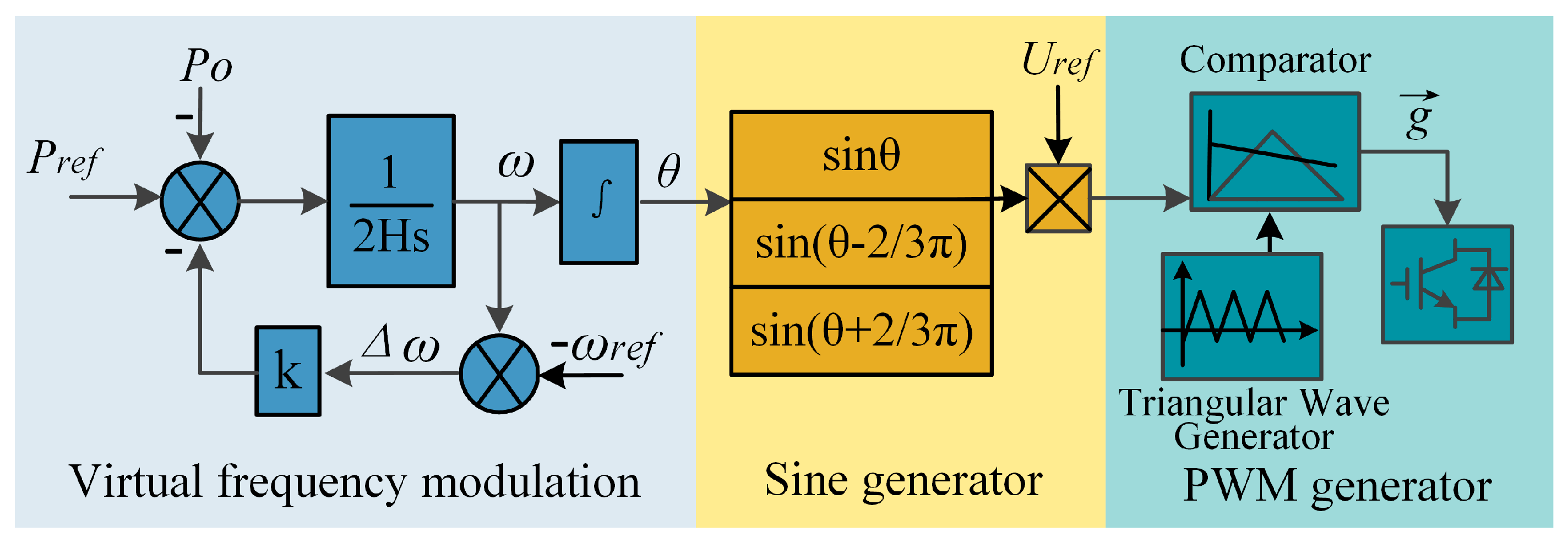
2.1. The VSG Control Scheme of IIDG
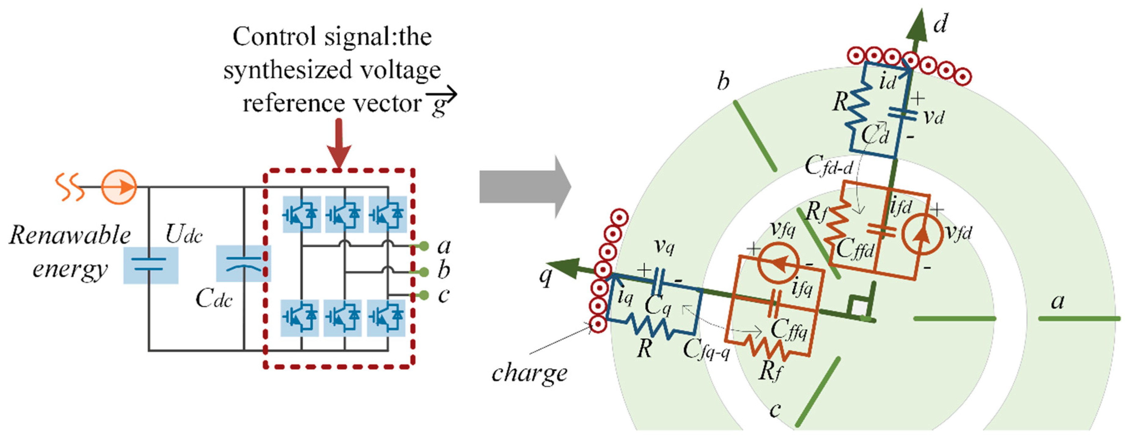
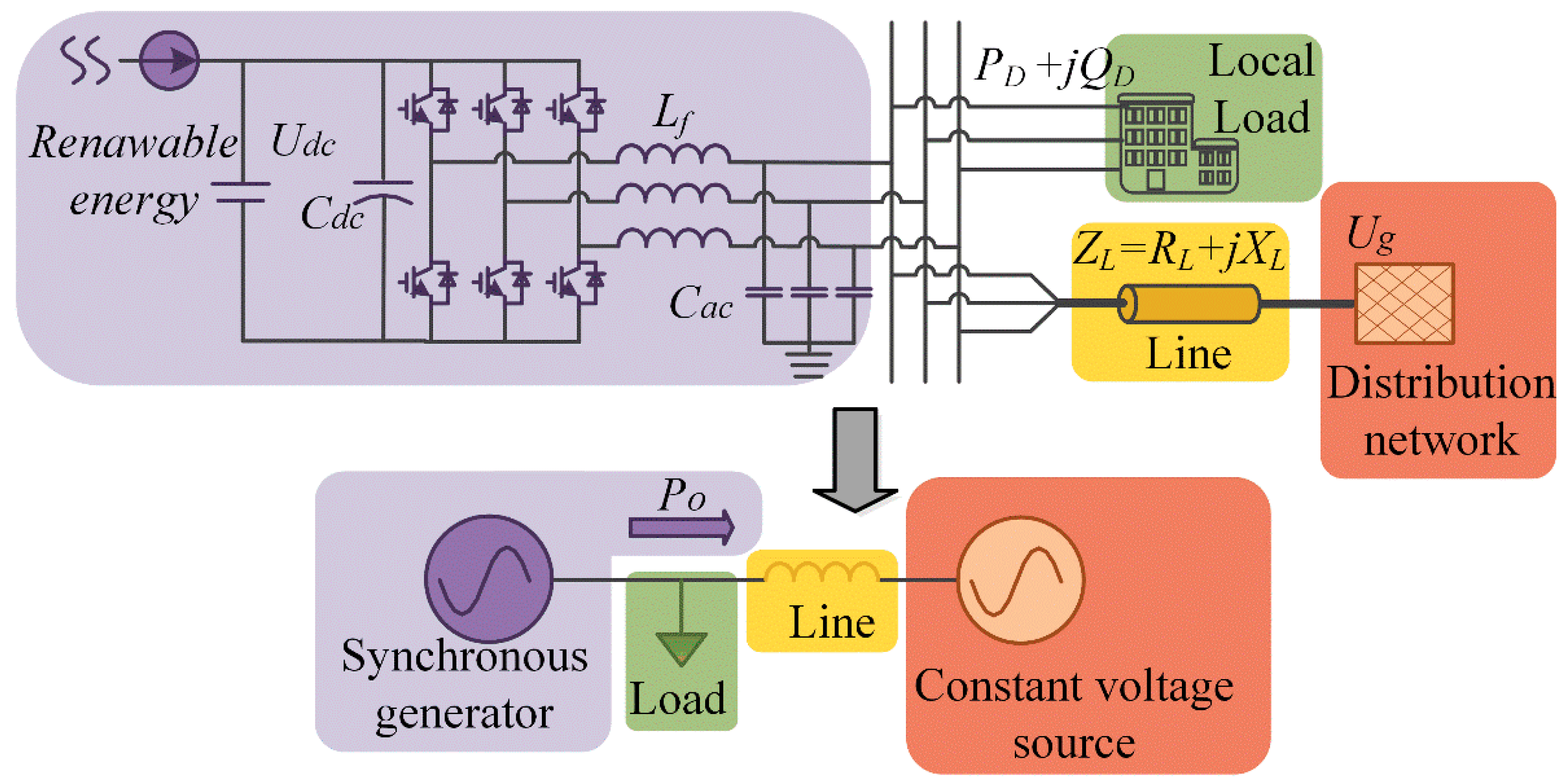
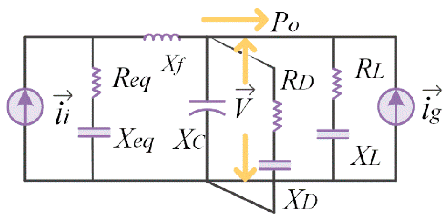
2.2. VSG-IIDG Equivalent Electrostatic Machine Model
3. The Nonlinear Mathematical Model of VSG-IIDG
4. Lyapunov Function Construction and the Stability Domain Determination
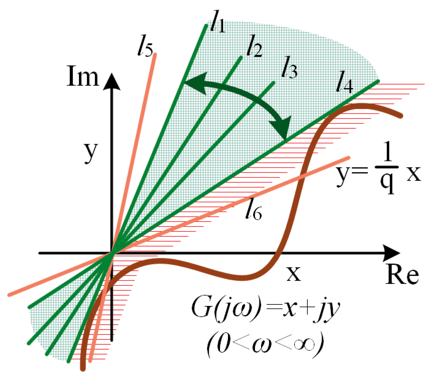
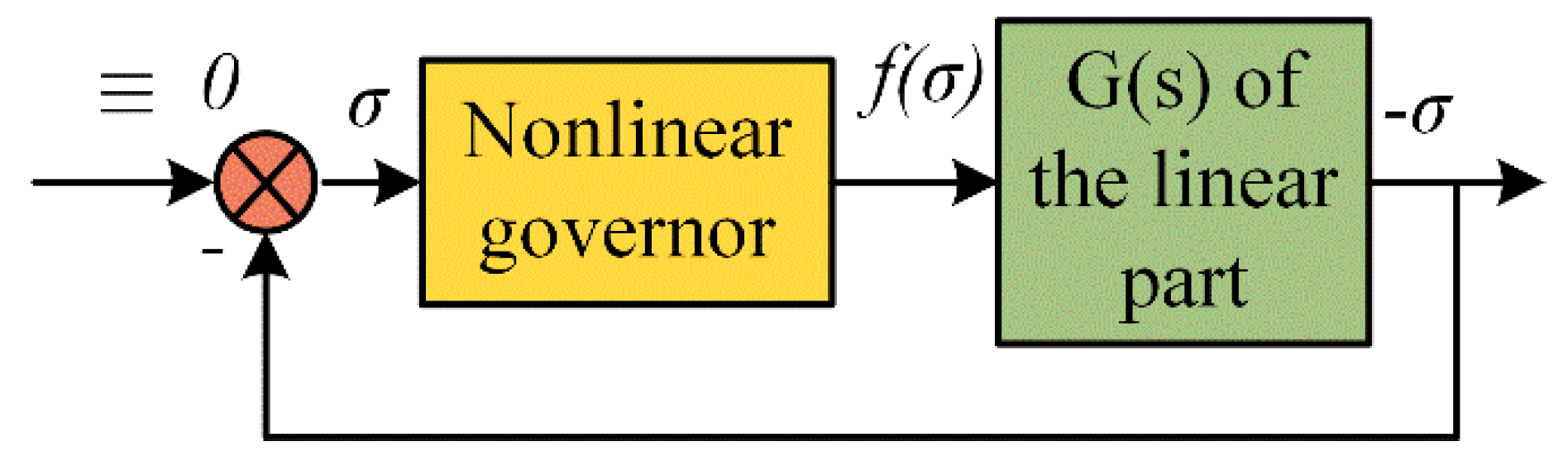
4.1. Popov stability Criterion
4.2. Lyapunov Function
- (a)
- Define the function as:where:
- (b)
- Factorize as: . Hence is:
- (c)
- Define the leading coefficient of the polynomial in ascending powers when in a . Then define a vector u with its components being the coefficients of the polynomial in ascending powers. Here the vector u reduces to a scalar in the VSG-IIDG model:
- (d)
- Figure out the symmetric positive definite matrix by solving the Lyapunov matrix equation:Here the Lyapunov matrix equation reduces to the scalar equation so that:
- (e)
- Get the Lyapunov function:
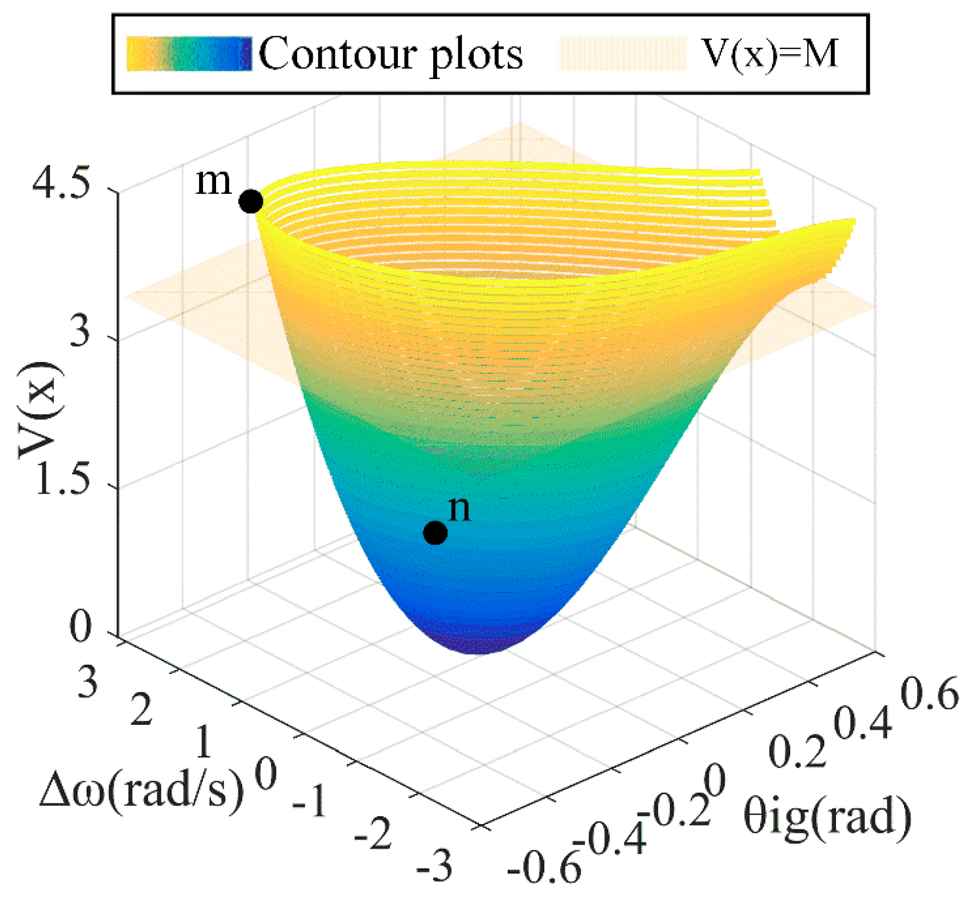
4.3. Lyapunov-Based Large Signal Stability Domain
5. Study Cases
5.1. Parameters of the Simulation Case
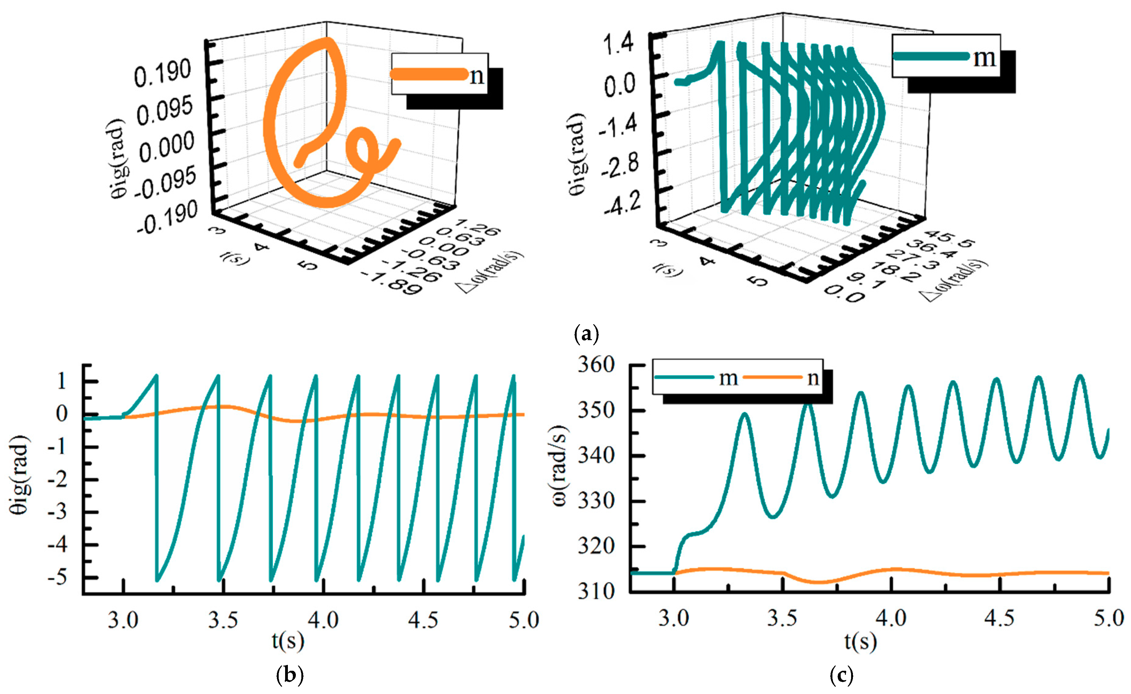
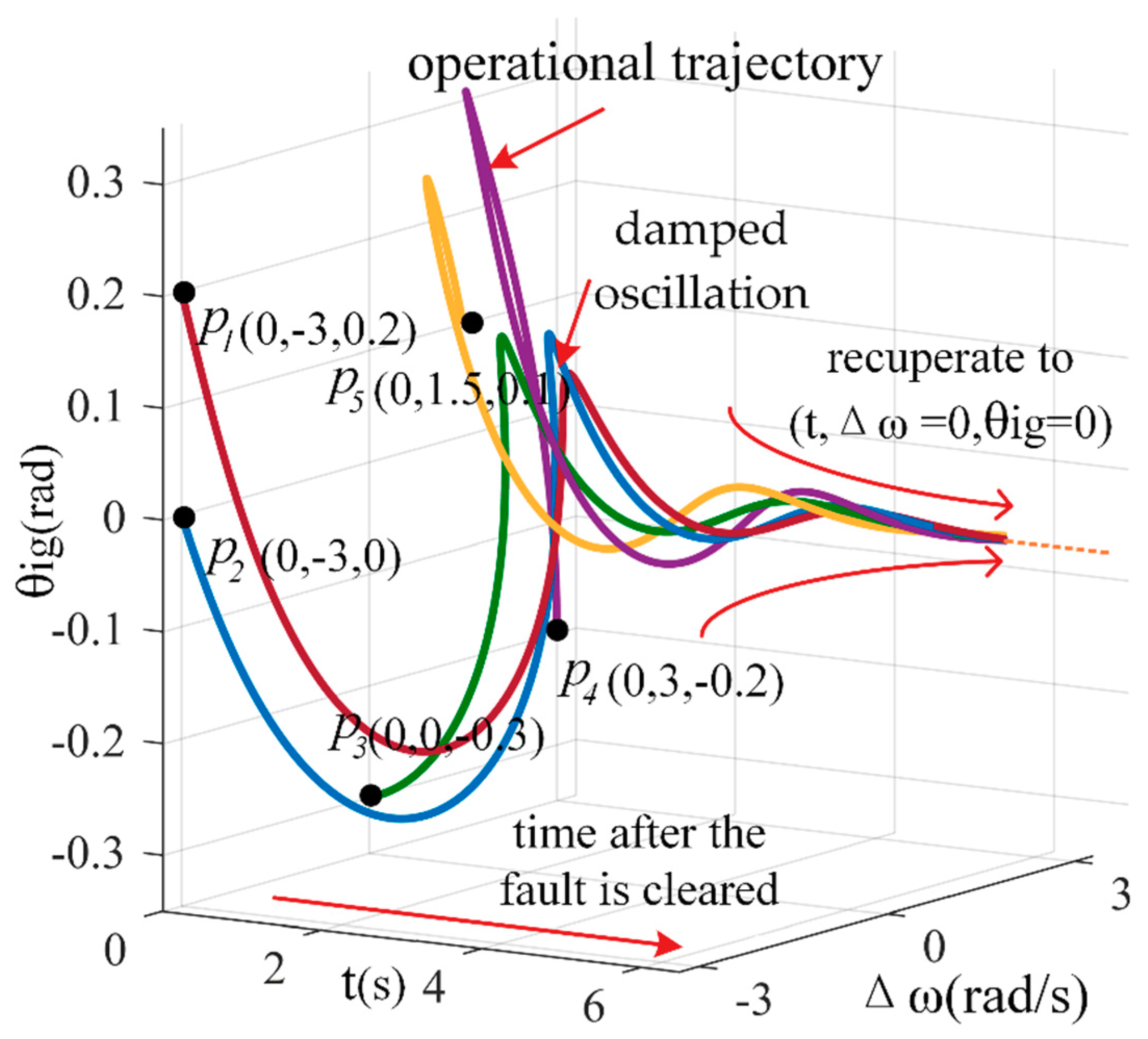
5.2. Large Signal Stability Analysis of the VSG-IIDG
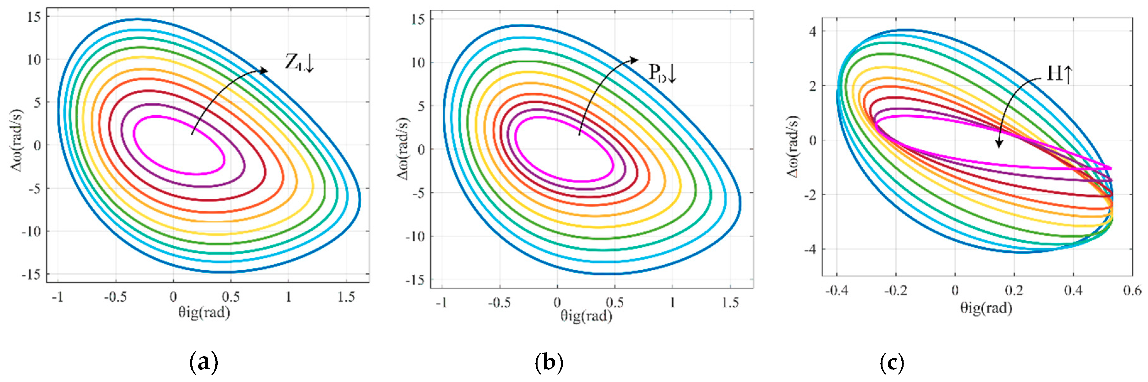
5.3. The Impact of Parameters on the Stability Domain
5.4. Sensitivity Analysis of Parameters
6. Conclusions
- (1)
- The nonlinear mathematical model of the VSG-IIDG is established. The equivalent model of electrostatic machine is applied. Both the electrical parts and control signals are taken into account. This nonlinear model can be an analytical tool for the study of large signal stability.
- (2)
- A Lyapunov function is derived based on Popov’s theory to determine the stability of IIDG. By comparing the transient energy of the post-fault system with the critical energy, this Lyapunov-based method has a distinct computational advantage.
- (3)
- The stability domain is depicted and the large signal stability mechanism of VSG-IIDGs is revealed. The stability domain quantifies the magnitude of the deviation that the system can tolerate. The impacts and sensitivity analysis of parameters on the stability domain are presented. The results indicate that large disturbances may lead to instability of the VSG-IIDG with deviation and oscillation of angular frequency. The VSG-IIDG tends to instability with larger load power and cable impedance or smaller virtual inertia.
Author Contributions
Funding
Conflicts of Interest
Nomenclature
| the power angle of the IIDG | |
| the power angle difference between and | |
| the equilibrium point | |
| the power angle of the common coupling point of VSG-IIDG | |
| ω | virtual angular frequency |
| angular frequency reference | |
| the angular frequency difference between ω and | |
| ,, | filtering capacitance of VSG-IIDG and the relative reactance and admittance |
| capacitance of the DC link of VSG-IIDG | |
| H | virtual inertia of the VSG-IIDG |
| ,,,, | inductor, resistance, reactance, admittance, and impedance of the cable |
| ,, | filtering inductor of VSG-IIDG and the relative reactance and admittance |
| M | critical stability energy |
| ,,,, | active power, reactive power, equivalent resistance, reactance, and admittance of the local load |
| Po | output active power measurement of the IIDG |
| active power reference of the IIDG | |
| ,, | the equivalent resistance, reactance, and admittance of the equivalent IIDG current source |
| the area of stability domain | |
| voltage at the DC link of VSG-IIDG | |
| voltage at the point of common coupling | |
| , | average values of voltage modulation for the duty cycle in d and q axis |
| the synthesized voltage reference vector in VSG control | |
| k | the damping factor of VSG-IIDG |
| the sensitivity | |
| q | Popov coefficient |
Appendix A
References
- Shuai, Z.; Sun, Y.; Shen, Z.J.; Tian, W. Microgrid stability: Classification and a review. Renew. Sustain. Energy Rev. 2016, 58, 167–179. [Google Scholar] [CrossRef]
- Soni, N.; Doolla, S.; Chandorkar, M.C. Improvement of Transient Response in Microgrids Using Virtual Inertia. IEEE Trans. Power Deliv. 2013, 28, 1830–1838. [Google Scholar] [CrossRef]
- Liu, J.; Miura, Y.; Bevrani, H. Enhanced Virtual Synchronous Generator Control for Parallel Inverters in Microgrids. IEEE Trans. Smart Grid 2017, 8, 2268–2277. [Google Scholar] [CrossRef]
- Chen, L.; Wang, R.; Zheng, T. Optimal Control of Transient Response of Virtual Synchronous Generator Based on Adaptive Parameter Adjustment. Proc. CSEE 2016, 11, 5724–5731. [Google Scholar]
- Zhang, X.; Zhu, D.; Xu, H. Review of Virtual Synchronous Generator Technology in Distributed Generation. J. Power Supply 2012, 10, 1–6. [Google Scholar]
- Mehrasa, M.; Godina, R.; Pouresmaeil, E.; Vechiu, I.; Rodríguez, R.L.; Catalão, J.P. Synchronous active proportional resonant-based control technique for high penetration of distributed generation units into power grids. Presented at the IEEE Pes Innovative Smart Grid Technologies Conference Europe, Torino, Italy, 26–29 September 2017; pp. 1–6. [Google Scholar]
- Pouresmaeil, E.; Mehrasa, M.; Godina, R. Double synchronous controller for integration of large-scale renewable energy sources into a low-inertia power grid. Presented at the IEEE Pes Innovative Smart Grid Technologies Conference Europe, Torino, Italy, 26–29 September 2017; pp. 1–6. [Google Scholar]
- D’Arco, S.; Suul, J.A.; Fosso, O.B. A virtual synchronous machine implementation for distributed control of power converters in Smart Grids. Electr. Power Syst. Res. 2015, 122, 180–197. [Google Scholar] [CrossRef]
- Meng, J.; Wang, Y.; Shi, X. Control strategy and parameter analysis of distributed inverter based on virtual synchronous generator. Trans. China Electrotech. Soc. 2014, 29, 1–10. [Google Scholar]
- Du, Y.; Su, J.; Zhang, Z. A mode adaptive FM control method for microgrid. China J. Electr. Eng. 2013, 33, 67–75. [Google Scholar]
- Mehrasa, M.; Pouresmaeil, E.; Zabihi, S.; Vechiu, I.; Catalão, J.P. A multi-loop control technique for the stable operation of modular multilevel converters in HVDC transmission systems. Int. J. Electr. Power Energy Syst. 2018, 96, 194–207. [Google Scholar] [CrossRef]
- Cheng, C.; Yang, H.; Zeng, Z. Adaptive control method of rotor inertia for virtual synchronous generator. Autom. Electr. Power Syst. 2015, 19, 82–89. [Google Scholar]
- Huang, L.; Xin, H.; Huang, W. Quantitative analysis method of frequency response characteristics of power system with virtual inertia. Autom. Electr. Power Syst. 2018, 42, 31–38. [Google Scholar]
- Zhu, S.; Liu, K.; Qin, L. A review of transient stability analysis for power electronic systems. Proc. Chin. Acad. Electr. Eng. 2017, 37, 3948–3962. [Google Scholar]
- Kabalan, M.; Singh, P.; Niebur, D. Large Signal Lyapunov-Based Stability Studies in Microgrids: A Review. IEEE Trans. Smart Grid 2017, 8, 2287–2295. [Google Scholar] [CrossRef]
- Mehrasa, M.; Adabi, M.E.; Pouresmaeil, E. Direct Lyapunov control (DLC) technique for distributed generation (DG) technology. Electr. Eng. 2014, 96, 309–321. [Google Scholar] [CrossRef]
- Mehrasa, M.; Pouresmaeil, E.; Catalao, J.P.S. Direct Lyapunov Control Technique for the Stable Operation of Multilevel Converter-Based Distributed Generation in Power Grid. Emerg. Sel. Top. Power Electr. 2014, 2, 931–941. [Google Scholar] [CrossRef]
- Liu, Y.; Chen, J.; Hou, X. Dynamic frequency stabilization control strategy for microgrid based on the adaptive virtual inertial system. Autom. Electr. Power Syst. 2018, 42, 75–82. [Google Scholar] [CrossRef]
- Alipoor, J.; Miura, Y.; Ise, T. Power system stabilization using a virtual synchronous generator with alternating moment of inertia. IEEE J. Emerg. Sel. Top. Power Electr. 2015, 3, 451–458. [Google Scholar] [CrossRef]
- Andrade, F.; Kampouropoulos, K.; Romeral Martínez, J.L.; Vasquez Quintero, J.C.; Guerrero, J.M. Study of large-signal stability of an inverter-based generator using a Lyapunov function. Presented at the 40th Annual Conference of the IEEE Industrial Electronics Society, Dallas, TX, USA, 29 October–1 November 2014; pp. 1840–1846. [Google Scholar]
- Gao, F.; Iravani, M.R. A Control Strategy for a Distributed Generation Unit in Grid-Connected and Autonomous Modes of Operation. IEEE Trans. Power Deliv. 2008, 23, 850–859. [Google Scholar]
- Andrade, F.A.; Romeral, L.; Cusido, J. New model of a converter-based generator using electrostatic synchronous machine concept. IEEE Trans. Energy Convers. 2014, 29, 344–353. [Google Scholar]
- Pai, M.A.; Mohan, M.A.; Rao, J.G. Power System Transient Stability: Regions Using Popov’s Method. IEEE Trans. Power Appl. Syst. 1970, PAS-89, 788–794. [Google Scholar] [CrossRef]
- Kalman, R.E. Liapunov functions for the problem of Lur’e solving (8b): In automatic control. Proc. Natl. Acad. Sci. USA 1963, 49, 201–205. [Google Scholar] [CrossRef] [PubMed]
- Walker, J.A.; McClamroch, N.H. Finite regions of attraction for problem of Lur’e. Intern. J. Control 1967, 6, 331–336. [Google Scholar] [CrossRef]
- Wang, X.; Jiang, H.; Liu, H. Summary of the research on virtual synchronous generator grid connection stability. North China Power Technol. 2017, 9, 14–21. [Google Scholar]
- Renedo, J.; GarcíA-Cerrada, A.; Rouco, L. Active power control strategies for transient stability enhancement of AC/DC grids with VSC-HVDC multi-terminal systems. IEEE Trans. Power Syst. 2016, 31, 4595–4604. [Google Scholar] [CrossRef]
- Hu, T. A nonlinear-system approach to analysis and design of power-electronic converters with saturation and bilinear terms. IEEE Trans. Power Electr. 2011, 26, 399–410. [Google Scholar] [CrossRef]
- He, Y.; Wen, Z.; Wang, F. Analysis of Power System; The Second Volume; Huazhong University of Science and Technology Press: Wuhan, China, 1985. [Google Scholar]
- Fouad, A.A.; Vittal, V. Power System Transient Stability Analysis Using the Transient Energy Function Method; Prentice Hall: Upper Saddle River, NJ, USA, 1992. [Google Scholar]


| Step 1 | Input the parameters: voltage, current, control parameters as H, k, etc. |
| Step 2 | Obtain the expression of output power as Equation (27) |
| Step 3 | Calculate the equilibrium point as Equation (4) |
| Step 4 | Establish Lyapunov function V() as Equation (18) |
| Step 5 | Figure out the critical stability energy M as Equation (19) |
| Step 6 | If V() < M, the system is large signal stable |
| Parameters | Value |
|---|---|
| DC voltage | 1 kV |
| DC capacitance | 100 μF |
| Filtering capacitance | 400 μF |
| Filtering impedance | 1 mH |
| AC voltage | 311 V |
| Resistance of cable | 0.2 |
| Reactance of cable | 1 mH |
| Power of load | 300 kW + j100 kVar |
| Virtual inertia H | 0.15 |
| Damping factor k | 0.01 |
| Load Power | Cable Impedance | Virtual Inertia H | Stability |
|---|---|---|---|
| 0.3 | 0.2 + j0.314 | 0.15 | stable |
| 0.6 | 0.2 + j0.314 | 0.15 | stable |
| 1 | 0.2 + j0.314 | 0.15 | unstable |
| 0.3 | 0.5 + j0.785 | 0.15 | stable |
| 0.3 | 1 + j1.57 | 0.15 | unstable |
| 0.3 | 0.2 + j0.314 | 0.5 | stable |
| 0.3 | 0.2 + j0.314 | 2 | unstable |
| (MW) | 0.1 | 0.3 | 0.5 | 0.7 | 0.9 |
| Sensitivity | −4.991 | −4.981 | −4.701 | −4.687 | −4.295 |
| (Ω) | 0.2 + j0.314 | 0.4 + j0.628 | 0.6 + j0.942 | 0.8 + j1.256 | 1 + j1.57 |
| Sensitivity | −5.661 | −5.508 | −5.138 | −4.037 | −4.011 |
| H | 0.1 | 0.5 | 1 | 1.5 | 2 |
| Sensitivity | −1.980 | −2.256 | −3.007 | −4.751 | −5.124 |
© 2018 by the authors. Licensee MDPI, Basel, Switzerland. This article is an open access article distributed under the terms and conditions of the Creative Commons Attribution (CC BY) license (http://creativecommons.org/licenses/by/4.0/).
Share and Cite
Li, M.; Huang, W.; Tai, N.; Yu, M. Lyapunov-Based Large Signal Stability Assessment for VSG Controlled Inverter-Interfaced Distributed Generators. Energies 2018, 11, 2273. https://doi.org/10.3390/en11092273
Li M, Huang W, Tai N, Yu M. Lyapunov-Based Large Signal Stability Assessment for VSG Controlled Inverter-Interfaced Distributed Generators. Energies. 2018; 11(9):2273. https://doi.org/10.3390/en11092273
Chicago/Turabian StyleLi, Meiyi, Wentao Huang, Nengling Tai, and Moduo Yu. 2018. "Lyapunov-Based Large Signal Stability Assessment for VSG Controlled Inverter-Interfaced Distributed Generators" Energies 11, no. 9: 2273. https://doi.org/10.3390/en11092273
APA StyleLi, M., Huang, W., Tai, N., & Yu, M. (2018). Lyapunov-Based Large Signal Stability Assessment for VSG Controlled Inverter-Interfaced Distributed Generators. Energies, 11(9), 2273. https://doi.org/10.3390/en11092273