Stochastic Hybrid Estimator Based Fault Detection and Isolation for Wind Energy Conversion Systems with Unknown Fault Inputs

Abstract

In recent years, the wind energy conversion system (WECS) has been becoming the vital system to acquire wind energy. However, the high failure rate of WECSs leads to expensive costs for the maintenance of WECSs. Therefore, how to detect and isolate the faults of WECSs with stochastic dynamics is the pressing issue in the literature. This paper proposes a novel comprehensive fault detection and isolation (FDI) method for WECSs. First, a stochastic model predictive control (SMPC) controller is studied to construct the closed-loop system of the WECS. This controller is based on the Markov-jump linear model, which could precisely establish the stochastic dynamics of the WECS. Meanwhile, the SMPC controller has satisfied control performance for the WECS. Second, based on the closed-loop system with SMPC, the stochastic hybrid estimator (SHE) is designed to estimate the continuous and discrete states of the WECS. Compared with the existing estimators for WECSs, the proposed estimator is more suitable for WECSs since it considers both the continuous and discrete states of WECSs. In addition, the proposed estimator is robust to the fault input. Finally, with the proposed estimator, the comprehensive FDI method is given to detect and isolate the actuators’ faults of the WECS. Both the system status and the actuators’ faults can be detected by the FDI method and it can effectively quantify the actuators’ fault by the fault residuals. The simulation results suggest that the SHE could effectively estimate the hybrid states of the WECS, and the proposed FDI method gives satisfied fault detection performance for the actuators of the WECS.

1. Introduction

With the growing of the energy crisis and the awareness of human environmental protection, wind power is increasingly used as a green energy source [1]. Wind turbines are usually installed in harsh environments such as coastal areas, deserts, and mountainous areas. This means that the reliability of large wind turbine system operations need to be improved. However, in recent years, the accidents of wind turbines and power grid disturbances (such as voltage sag mitigation [2,3] to which wind energy conversion systems (WECSs) are highly sensitive) caused by loss of control in the design, manufacture, installation, operation and maintenance of intermediate links have threatened the safe operation of wind farms. The probability of failure of actuators and sensors is very high, and maintenance costs are enormous [4,5]. Therefore, fault detection and diagnosis of wind turbines have become a vital and stiff topic.

To realize the fault detection and isolation (FDI) of WECSs, the issue of how to construct the closed-loop control system is a prerequisite. The WECS is a complex stochastic switching nonlinear dynamic system, which is integrating mechanisms, electricity and liquid. Therefore, the traditional control methods have difficulty in achieving satisfactory performance [5]. In these features of WECSs, the stochastic switching, which is caused by the randomness of the wind, is the most important feature of the WECS. Notably, the stochastic switching feature can be represented as having the Markov jump characteristics, so the WECS can be described as a Markov jump linear system (MJLS). The Markov jump linear system is a nonlinear system that describes the system with uncertainty and disturbance as a Markov chain process. In 2012, Bernardini and Bemporad [6] proposed a scenario-based stochastic model predictive control for the stochastic Markov jump linear system. This kind of scenario-based stochastic model predictive control can be well applied to stochastic MJLSs. The main benefit of stochastic model predictive control is that it can make predictions with the full use of the statistical information of disturbance. Stochastic model predictive control (SMPC) has been used in many fields, such as drinking water networks [7], microgrids [8,9], electric vehicles [10], and so forth [11,12]. Furthermore, the scenario-based stochastic model predictive control has rarely been applied to solve the optimal control problem of wind turbines under random wind speed [13].

With the closed-loop system, estimating the system states is needed by the FDI of WECSs. Scholars also have extensive and in-depth research on state estimation [14,15,16,17,18,19,20]. In the literature, the Kalman filter is the most commonly used method to estimate states [14]. For discrete-time state-space Markov models, Crisan [15] uses a sequential Monte Carlo method to design nested structure particle filters to approximate the posterior probability measure of the static parameters and the dynamic state variables of the system. Hu [16], based on the Markov chain Monte Carlo to Sequential Monte Carlo algorithm, propose a state space model with Bayesian online estimation method to derive the optimal Bayesian estimation. Notably, it is a significant issue in the literature to accurately locate faults for hybrid systems. Liu [21] designed the robust estimation algorithm for a typical hybrid system (the aircraft). In this paper, the control object is the wind turbines, and the control method is the more advanced and complicated SMPC.

A lot of research has been started in recent years for the fault diagnosis and isolation of wind turbines [22,23,24,25,26,27,28,29]. Karim [22] designed an observer scheme for FDI, which is integrated with a maximum-shift strategy and a time-varying Kalman filter for the additive and multiplicative measurement failures of voltage and current. Silvio [23] used fuzzy models to estimate fault residuals for diagnosis and isolation. Iury [24] uses data-driven methods for fault detection, and a fuzzy/Bayesian network to distinguish faults. However, current research works do not systematically consider the stochastic hybrid characteristics of wind turbines and do not estimate the continuous and discrete states of the wind turbine during fault diagnosis and isolation.

This work presents a new FDI method based on stochastic hybrid estimation for WECSs. First, the scenario-based SMPC controller is used to deal with the control problem of wind energy conversion systems. By extracting the probability information of wind speed, the Markov jump linearization model of the wind turbine can be constructed, so that the random switching characteristics of the wind turbine can be accurately described. With this model, the SMPC can be benefited from the probability information of the wind to achieve a better control performance. Second, this paper proposed a stochastic hybrid estimator that estimates the continuous state and the discrete states of WECSs with unknown fault inputs. The proposed estimator decouples the unknown fault inputs from the estimation error dynamics of the hybrid system. With this decoupling, it can guarantee that the estimation is not influenced by the fault input. At last, the comprehensive FDI method is used to detect and isolate the actuators’ faults of WECSs. The innovation of the FDI algorithm proposed in this paper is that it can accurately estimate both the continuous and discrete states of the WECS with unknown fault inputs. The principle is to construct the system fault residual based on the accurate estimation of the proposed estimator and use the statistical decision tool to realize fault detection and isolation. The continuous state estimation of the system can be obtained by stochastic hybrid estimation, and the discrete state estimation of the system can be derived by Bayesian theory. The simulation results show that the SMPC controller has good control performance for the WECS, and the FDI algorithm has good fault detection and isolation effect. Both the fault amplitude and the fault occurrence can be effectively estimated by the proposed method.

This paper has been divided into five parts. The first part deals with the SMPC controller design in Section 2; the second part focuses on the stochastic hybrid estimation for WECSs in Section 3; the third part presents the comprehensive FDI algorithm for WECSs in Section 4; the fourth part is the simulation verification of the SMPC controller and the FDI method shown in Section 5; the last part is the conclusion, which gives a brief summary in Section 6.

2. Scenario-Based SMPC for Wind Energy Conversion Systems

To construct the closed-loop control system of a WECS, the SMPC controller is studied to implement this procedure in this section. The Markov jump model of the WECS is briefly given first. With this model, the SMPC controller is used to realize the closed-loop control of the WECS.

2.1. Markov Chain Transition Matrix of the Wind Speed

For a Markov chains theory applied to wind speed time series data, the one-step (first-order) probability transition matrix $P$ of the wind speed includes the statistical information of the discrete wind speed time series [30]. The one-step Markov transition matrix of the wind speed can be estimated by a statistical method. In order to obtain the Markov chain transition matrix of the wind speed, the wind speed is discretized into $v_t$, $t\in \left(0,1,2,\dots ,T\right)$, then divided into different intervals according to the wind speed (Figure 1) [5]. The state transition probability $p_{ij}$ of the wind speed is the probability that the state of wind speed is $S_i$ in time $t$ ($\mathrm{i}.\mathrm{e}.,v_t=S_i$), and is $S_j$ in time $t+1\left(\mathrm{i}.\mathrm{e}.,v_{t+1}=S_j\right)$, $t\in \left(0,T-1\right)$:

$$p_{ij}=Pr\left\{v_{t+1}=S_j|v_t=S_i\right\}$$

(1)

Let $n_{ij}$ denote the number of wind speeds that are in state $S_i$ at period $t$ and are in state $S_j$ at period $t+1$, and then:

$$p_{ij}=\frac{n_{ij}}{{{\displaystyle \sum }}_{j=1}^3{n}_{ij}}$$

(2)

The one-step (first-order) transition matrix $P\left(P\in R^{3\times 3}\right)$ could be represented as:

$$P=\left[\begin{array}{ccc}{p}_{11}& p_{12}& p_{13}\\ p_{21}& p_{22}& p_{23}\\ p_{31}& p_{32}& p_{33}\end{array}\right]$$

(3)

where $p_{ij}\ge 0,{{\displaystyle \sum }}_{j=1}^3{p}_{ij}=1,i,j=1,\cdots ,3$ [31].

2.2. Modeling of the WECS

The physical structure of a wind energy conversion system is presented as Figure 2, where the system inputs are the generator torque reference $T_{gref}\left(t\right)$ and the pitch angle reference ${\beta }_{ref}\left(t\right)$. Wind speed $v\left(t\right)$ is the disturbance. Generator power $P_g\left(t\right)$ and generator speed ${\omega }_g\left(t\right)$ are the outputs of the WECS.

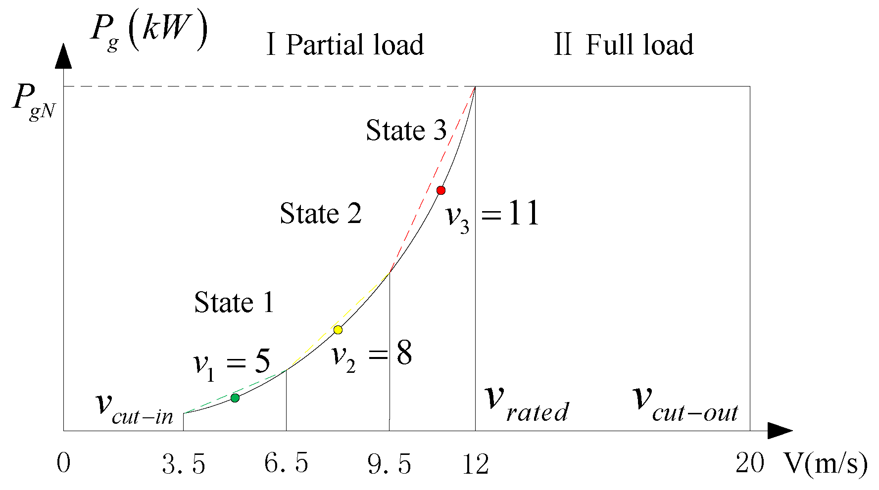
Since the operation of the WECS has different working domains (mainly partial load and full load), the physical model of the WECS can be linearized for a specified working point in the different working domains, as shown in Figure 1.

The state space dynamic model (4) of the wind energy conversion system can be obtained assembly by mechanism modeling, which is shown as follows, and the derivation process of the WECS dynamic model can be found in the previous work [5].

$$\left[\begin{array}{c}{\dot{T}}_g\\ \dot{\beta }\\ \ddot{\beta }\\ {\dot{\omega }}_g\\ {\dot{\omega }}_r\\ {\dot{\omega }}_1\\ {\dot{\omega }}_2\end{array}\right]=\left[\begin{array}{ccccccc}{A}_{11}& 0& 0& 0& 0& 0& 0\\ 0& 0& I& 0& 0& 0& 0\\ 0& A_{54}& A_{55}& 0& 0& 0& 0\\ a_{71}& 0& 0& a_{77}& \frac{B_{dt}}{N_g{J}_g}& 0& 0\\ 0& a_{84}& 0& \frac{B_{dt}}{N_g{J}_r}& a_{88}& 0& 0\\ 0& 0& 0& 0& 0& 0& 1\\ 0& 0& 0& 0& 0& -a_1& -a_2\end{array}\right]\left[\begin{array}{c}{T}_g\\ \beta \\ \dot{\beta }\\ {\omega }_g\\ {\omega }_r\\ {\omega }_1\\ {\omega }_2\end{array}\right]+\left[\begin{array}{cc}{B}_{11}& 0\\ \begin{array}{c}0\\ \begin{array}{c}0\\ 0\\ \begin{array}{c}0\\ 0\\ 0\end{array}\end{array}\end{array}& \begin{array}{c}0\\ \begin{array}{c}{B}_{42}\\ 0\\ \begin{array}{c}0\\ 0\\ 0\end{array}\end{array}\end{array}\end{array}\right]\left[\begin{array}{c}{T}_{gref}\\ {\beta }_{ref}\end{array}\right]+\left[\begin{array}{c}0\\ 0\\ 0\\ 0\\ e_{81}\\ 0\\ 0\end{array}\right]v_m+\left[\begin{array}{c}0\\ 0\\ 0\\ 0\\ e_{81}\\ 0\\ a_3\end{array}\right]e$$

(4)

where, $v\left(t\right)=v_m\left(t\right)+e,v_m\left(t\right)$ is the mean wind speed, $e\in \mathcal{N}\left(0,1\right)$ is the Gaussian white noise, ${\omega }_1,{\omega }_2$ are the augmented state variables when $e$ is approximated as a linear filter [32], and $A_{11}=-\frac{1}{{\tau }_g},A_{54}=-{\omega }_n^2,A_{55}=-2\xi {\omega }_n,a_{71}=-\frac{1}{J_g},a_{77}=-\left(\frac{{\eta }_{dt}{B}_{dt}}{J_g{N}_g^2}+\frac{B_g}{J_g}\right),a_{84}=\frac{1}{3J_r}\frac{\partial T_a}{\partial \beta },a_{88}=-\frac{B_{dt}+B_r}{J_r}+\frac{1}{J_r}\frac{\partial T_a}{\partial {\omega }_r},B_{11}=\frac{1}{{\tau }_g},B_{42}={\omega }_n^2,e_{81}=\frac{1}{3J_r}\frac{\partial T_a}{\partial v_r}.\frac{\partial T_a}{\partial v_r},\frac{\partial T_a}{\partial {\omega }_r}$ and $\frac{\partial T_a}{\partial \beta }$ are the linearized coefficients in different wind speed working points.

To obtain the parameters of the model (4), the power coefficient $C_p\left(\lambda ,\beta \right)$ of the WECS is a key value [33], which determined by the pitch angle $\beta$ and the tip-speed ratio $\lambda$.

$$C_p\left(\lambda ,\beta \right)=0.22\left(\frac{116}{{\lambda }_t}-0.4\beta -5\right)e^{\frac{-12.5}{{\lambda }_t}}$$

(5)

$$\frac{1}{{\lambda }_t}=\frac{1}{\lambda +0.08\beta }-\frac{0.035}{{\beta }^3+1}$$

(6)

The relationship of $C_p,$ $\lambda ,\beta$ and the wind speed is shown in Figure 3.

A tracking control algorithm with augmented state variables in model (4) [34] is implemented. It has been used in the previous studies [5], which can be described as follows:

Consider model (4) as a continuous-time linear system

$$\dot{x}=Ax+Bu+D+D1\times e,y=Cx,x\left(t_0\right)=x_0$$

(7)

where, $C=\left[\begin{array}{ccc}0& 0& 0\\ -45& 0& 0\end{array}\begin{array}{ccc}1& 0& 0\\ 0.5& 0& 0\end{array}\begin{array}{c}0\\ 0\end{array}\begin{array}{cc}0& 0\\ 0& 0\end{array}\right]$, $y={\left[\begin{array}{cc}{w}_g& P_g\end{array}\right]}^T$. Let $N_r$ be the output reference, then the augmented state is

$${\dot{x}}^{ref}=N_r-y=N_r-Cx$$

(8)

Then the augmented state equation can be defined as

$${\dot{x}}_{{\displaystyle \sum }}=A_{{\displaystyle \sum }}{x}_{{\displaystyle \sum }}+B_{{\displaystyle \sum }}u+D_{{\displaystyle \sum }}+D{1}_{{\displaystyle \sum }}\times e+N_{{\displaystyle \sum }},y=Cx,x_{{\displaystyle \sum }0}\left(t_0\right)=x_{{\displaystyle \sum }0}$$

(9)

where

$$x_{{\displaystyle \sum }}=\left[\begin{array}{c}x\\ x^{ref}\end{array}\right],A_{{\displaystyle \sum }}=\left[\begin{array}{cc}A& 0\\ -C& 0\end{array}\right],B_{{\displaystyle \sum }}=\left[\begin{array}{c}B\\ 0\end{array}\right],D_{{\displaystyle \sum }}=\left[\begin{array}{c}D\\ 0\end{array}\right],D{1}_{{\displaystyle \sum }}=\left[\begin{array}{c}D1\\ 0\end{array}\right],N_{{\displaystyle \sum }}=\left[\begin{array}{c}0\\ N_r\end{array}\right]$$

(10)

Discretizing and linearizing model (9) at three working points in which the wind speeds are 5, 8 and 11 m/s, respectively. Then, it can obtain the WECS discrete-time linear system:

$$\begin{array}{c}x\left(k+1\right)=A\left(w\left(k\right)\right)x\left(k\right)+B\left(w\left(k\right)\right)u\left(k\right)+D\left(w\left(k\right)\right)+D1\left(w\left(k\right)\right)e\left(k\right)+Iw\times yr\left(k\right)\\ y\left(k\right)=Cx\left(k\right)\end{array}$$

(11)

where $I_w={\left[\begin{array}{ccc}0& 0& 0\\ 0& 0& 0\end{array}\begin{array}{ccc}0& 0& 0\\ 0& 0& 0\end{array}\begin{array}{c}0\\ 0\end{array}\begin{array}{cc}1& 0\\ 0& 1\end{array}\right]}^T$, $k\in N$ is the time index $yr\left(k\right)={\left[\begin{array}{cc}{w}_{gref}& P_{gref}\end{array}\right]}^T$, is the output reference, $x\left(k\right)\in R^{n_x}$ is the state, $y\left(k\right)={\left[\begin{array}{cc}{w}_g& P_g\end{array}\right]}^T$ is the output, $u\left(k\right)\in R^{n_u}$ is the input, $e\left(k\right)\in \mathcal{N}\left(0,1\right)$, $w\left(k\right)\in W$ is the disturbance, and $W=\left\{1,2,3\right\}$ $\subset$ R is a finite set. $A\left(w\left(k\right)\right)$, $B\left(w\left(k\right)\right)$, $D\left(w\left(k\right)\right)$ and $D1\left(w\left(k\right)\right)$ are the WECS model matrixes matching the three operation states of the system $S_i,i=\left\{1,2,3\right\}$, which seen in Appendix A.

2.3. Wind Energy Conversion System Fault Model with Unknown Fault Inputs

This paper considers the unknown fault inputs $u_F\left(k\right)$, which is added simultaneously with the normal input $u\left(k\right)$ to the actuator. Consider the following discrete stochastic model of a wind energy conversion system with unknown fault inputs:

$$\begin{array}{c}x\left(k+1\right)=A\left(w\left(k\right)\right)x\left(k\right)+B\left(w\left(k\right)\right)u\left(k\right)+F\left(w\left(k\right)\right)u_F\left(k\right)+D\left(w\left(k\right)\right)+D1\left(w\left(k\right)\right)e\left(k\right)+Iw\times yr\left(k\right)\\ y\left(k\right)=Cx\left(k\right)\end{array}$$

(12)

where $F\left(w\left(k\right)\right)=B\left(w\left(k\right)\right)$. It should be noticed that $u_F\left(k\right)$ is not considered in the design of SMPC, for $u_F\left(k\right)$ are the unknown fault inputs. In order to investigate stochastic estimation and FDI, we make the following assumptions for the unknown fault inputs:

Assumption 1.

$F\left(w\left(k\right)\right)$ is a full column rank matrix [35].

Assumption 1 ensures that the fault diagnosis and isolation algorithm (FDI) of this paper has a solution.

Assumption 2.

The $F\left(w\left(k\right)\right)$ column rank does not exceed the $C$ row rank [36,37].

Assumption 2 can be expressed equivalently that $CF\left(w\left(k\right)\right)$ is a full column rank matrix. In the following, it will be shown that Assumption 2 can guarantee the presence of a state estimator that is robust to the fault input. In practical applications, Assumption 2 can be achieved by adding sensors.

2.4. Scenario-Based SMPC Design

The optimization objective function of the stochastic model predictive control can be expressed as follow:

$$\begin{array}{c}min\\ u\end{array}{E}_w\left[{\displaystyle \sum }_{j\in T\backslash (N_1{\displaystyle \cup }s)}{\left(x_j-x_r\right)}^{T}Q\left(x_j-x_r\right)+{\displaystyle \sum }_{j\in T\backslash S}{u}_j^{T}R{u}_j\right]$$

(13)

where $E_w$ is the expectation, $x_r$ is the state reference value, $x_j$ is the output of scenario $j$, and $u_j$ is the input of scenario $j$. The construction of the scenario tree can be detailed with reference to [5].

Solving problem (13), the paper systematically considers the realization of the scenarios and their probability to minimize the expectation (Exp) performance index of the state and input. More clearly stated: (1) the normal expectation objective function of scenario $j$, multiplied by its realization probability, gets the expectation $E_{wj}\left(j\in \left\{1,2,\dots s\right\}\right)$ of the scenario $j$; (2) Accumulating all the scenarios’ expectations $E_{wj}$ to get the entire scenario-tree’s expectation $E_w$. By the above two steps, a concise solution method of the problem (13) can be obtained. In this way, the uncertain SMPC problem (13) can be simplified to a deterministic MPC problem. At time $k$, based on the scenario tree introduced in [5], the stochastic model predictive control problem with expectation performance index is defined as:

$$\begin{array}{l}\begin{array}{c}min\\ u\end{array}{\displaystyle {\displaystyle \sum }_{j\in T\backslash \left(T_1{\displaystyle \cup }S\right)}}{\pi }_i{\left(x_j-x_r\right)}^{T}Q\left(x_j-x_r\right)+{\displaystyle {\displaystyle \sum }_{j\in T\backslash S}}{\pi }_j{u}_j^{T}R{u}_j\\ s.t.\{\begin{array}{l}{x}_1=x\left(k\right)\hfill \\ \begin{array}{c}{x}_i=A\left(w\left(k\right)\right)x_{pre\left(i\right)}+B\left(w\left(k\right)\right)u_{pre\left(i\right)}+D\left(w\left(k\right)\right)\\ +D1\left(w\left(k\right)\right)e\left(k\right)+Iw\times yr\left(k\right),i\in T\backslash \left\{T_1\right\}\end{array}\hfill \\ G_{x}x\left(k\right)+G_{u}u\left(k\right)\le g,k=0,\dots ,N,\forall w\left(k\right)\in W\hfill \end{array}\end{array}$$

(14)

where ${\pi }_j$ is the realization probability of scenario $j,R$ and $Q$ are the weight matrixes, $x\left(k\right)$ is the current state of the system, and $x_i$ is the $i$-th step state. $G_x\in R^{n_x+n_u}$ and $G_u\in R^{n_x+n_u}$ are coefficient matrixes in state and input constraints. The fault is not considered in the predictive model in problem (14) because this paper considers the unknown actuator fault input. The problem (14) is a quadratic constrained quadratic programming problem. The system input $u_1$ of the root node $N_1$ can be obtained by the first component of the solution to the problem (14). The function (14) is a receding horizon optimization problem, and the current control law is given by online optimization.

Since the problem (14) is difficult to solve directly, it is necessary to construct a scenario tree of the stochastic model to convert problem (14) into a deterministic problem. The scenario-based stochastic model predictive control problem can be solved in two steps, as shown above. The predictive control problem of one of the scenarios is the ordinary model predictive control problem. Based on the solution of one scenario, simply multiply the $J^{*}\left(x_j\right)$ of each scenario $j$ by its disturbance to realize the probability ${\pi }_j$, thus obtaining the expectation $E_w{}_j,\left(j\in \left\{1,2,\dots ,s\right\}\right)$ of the scenario $j$. By accumulating the expectation $E_w{}_j$ of all the scenarios, the expectation $E_w$ of the entire scenario tree is obtained. The specific solution process can be expressed as:

$$\begin{array}{l}{J}^{*}\left(x\right)=\begin{array}{c}min\\ u\end{array}{\displaystyle {\displaystyle \sum }_{j\in T\backslash \left(N_1{\displaystyle \cup }S\right)}}{\pi }_j{\left(x_j-x_r\right)}^{T}Q\left(x_j-x_r\right)+{\displaystyle {\displaystyle \sum }_{j\in T\backslash S}}{\pi }_j{u}_j^{T}R{u}_j\\ ={}_u{}^{min}\{{\pi }_1{\left(x_1-x_r\right)}^{T}Q\left(x_1-x_r\right)+{\pi }_1{U}_1{\left(k\right)}^{T}R{U}_1\left(k\right)\\ +{\pi }_2{\left(x_2-x_r\right)}^{T}Q\left(x_2-x_r\right)+{\pi }_2{U}_2{\left(k\right)}^{T}R{U}_2\left(k\right)\\ +\dots \\ +{\pi }_s{\left(x_s-x_r\right)}^{T}Q\left(x_s-x_r\right)+{\pi }_s{U}_s{\left(k\right)}^{T}R{U}_s\left(k\right)\}\end{array}$$

(15)

where ${\pi }_j={{\displaystyle \prod }}_{i=1}^N{p}_{ij}$ ($p_{ij}$ is shown in Section 2.1) represents the realization probability of scenario $j$.

Let

$$\begin{array}{l}f{x}_j=(q{x}_j\times x\left(k\right)-q{r}_j\times x_r+q{d}_j\times Iw1+qd{1}_j\times \left(Iw1\times e\left(k\right)\right)\\ +qd{3}_j\times \left(Iw3\times yr\left(k\right)\right)),q{x}_j={\pi }_j{G}_{B_j}^{T}Q{G}_{A_j},q{r}_j=-{\pi }_j{G}_{B_j}^{T}Q,\\ q{d}_j={\pi }_j{G}_{B_j}^{T}Q{G}_{D_j},qd{1}_j={\pi }_j{G}_{B_j}^{T}Q{G}_{D{1}_j},qd{3}_j={\pi }_j{G}_{B_j}^{T}Q{G}_{D{3}_j},\\ U=\left[U_1;U_2;\dots U_s\right]\end{array}$$

(16)

The semicolon in $U$ stands for column arrangement.

In the same way as the solution of standard state space based model predictive control problem, problem (15) can be organized as:

$$\begin{array}{l}{J}^{*}\left(x\right)=\begin{array}{c}min\\ u\end{array}{\displaystyle {\displaystyle \sum }_{j\in T\backslash \left(N_1{\displaystyle \cup }S\right)}}{\pi }_j{\left(x_j-x_r\right)}^{T}Q\left(x_j-x_r\right)+{\displaystyle {\displaystyle \sum }_{j\in T\backslash S}}{\pi }_j{u}_j^{T}R{u}_j\\ =U{\left(k\right)}^{T}dia{g}_{j=1}^s\{{\pi }_j(G_{B_j}^{T}Q{G}_{B_j}+R)\}U\left(k\right)+2{\left[f{x}_1;f{x}_2;\dots f{x}_s\right]}^{T}U\left(k\right)\end{array}$$

(17)

where $diag$ is arranged in the form of a left diagonal. Let

$$Q_Z=dia{g}_{j=1}^s\{{\pi }_j(G_{B_j}^{T}Q{G}_{B_j}+R)\},fx=\left[f{x}_1;f{x}_2;\dots f{x}_s\right]$$

(18)

Problem (15) can be rewritten as:

$$\begin{gathered} J^{*}\left(x\right)=U{\left(k\right)}^T{Q}_{Z}U\left(k\right)+2f{x}^T\times U\left(k\right) \\ s.t.\{\begin{array}{l}{x}_1=x\left(k\right)\\ x_i=A\left(w\left(k\right)\right)x_{pre\left(i\right)}+B\left(w\left(k\right)\right)u_{pre\left(i\right)}+D\left(w\left(k\right)\right)\\ +D1\left(w\left(k\right)\right)e\left(k\right)+Iw\times yr\left(k\right),i\in T\backslash \left\{T_1\right\}\\ A{u}_j\times U_j\left(k\right)\le bu+C_{A_j}\times x\left(k\right)+C_{r_j}\times x_r+C_{D_j}\times Iw1\\ +C_{D{1}_j}\times \left(Iw1\times e\left(k\right)\right)+C_{D{3}_j}\times \left(Iw3\times yr\left(k\right)\right)\\ A{x}_j\times x_j\le bx\end{array} \end{gathered}$$

(19)

where $A{u}_j,bu,C_{A_j},C_{r_j},C_{D{1}_j},C_{D{3}_j},A{x}_{j}andbx$ are coefficient matrixes in input and state constraints of scenario $j$.

In this way, the SMPC’s Exp performance index (problem (14)) is solved as a quadratic programming (QP) problem (19).

3. Design of Stochastic Hybrid Estimator

In this section, we propose a stochastic hybrid estimator [21] for unknown faults (disturbances) of WECSs. The faults are arranged in combination, and the continuous and discrete states of the system are estimated separately. This approach will only require three designed filters. When the FDI algorithm in Section 4 determines that the system has failed, the user finds the discrete state of the system and the fault of the corresponding continuous state as needed.

3.1. The Problem of Stochastic Hybrid Estimation Algorithm

Combing the wind turbine discrete Markov jump linearization model (11) with the wind speed Markov state transition matrix $P\in R^{3\times 3}$ established in Section 2.1, the stochastic hybrid estimation problem can be described as the estimated system status. In order to estimate the state of the system, it is necessary to estimate the probability distribution of the discrete state of the system and then estimate the continuous state of the system that is not affected by the fault input.

This paper proposes a stochastic hybrid estimation algorithm for hybrid systems which is insensitive to actuators’ unknown fault inputs. Note that when the WECS operates in a discrete state, its characteristics are the same as those of linear time-invariant (LTI) systems $\{A\left(w\left(k\right)\right),B\left(w\left(k\right)\right),C,F\left(w\left(k\right)\right)|w\in W\}$. Therefore, a state estimator is designed for an LTI system.

Consider

$$\begin{array}{l}\widehat{x}\left(k+1\right)=A\left(w\left(k\right)\right)\widehat{x}\left(k\right)+B\left(w\left(k\right)\right)u\left(k\right)\hfill \\ +L\left(w\left(k\right)\right)\left[y\left(k+1\right)-CA\left(w\left(k\right)\right)\widehat{x}\left(k\right)-CB\left(w\left(k\right)\right)u\left(k\right)\right]\hfill \end{array}$$

(20)

$$r\left(k\right)=T\left(w\left(k\right)\right)\left[y\left(k+1\right)-CA\left(w\left(k\right)\right)\widehat{x}\left(k\right)-CB\left(w\left(k\right)\right)u\left(k\right)\right]$$

(21)

where $\widehat{x}\left(k\right)$ is the continuous state estimation, $w\left(k\right)$ is the discrete state, and $L\left(w\left(k\right)\right)$ is the parameter matrix to be designed. For the sake of easy understanding, $L\left(w\left(k\right)\right)$ and $T\left(w\left(k\right)\right)$ are regarded as the fixed matrix of the state $w$; from the next section, $L\left(w\left(k\right)\right)$ and $T\left(w\left(k\right)\right)$ are the time-varying matrix, which needs to be updated online with the simulation. Define the estimation error as

$$es\left(k\right):=x\left(k\right)-\widehat{x}\left(k\right)$$

(22)

Combining model (12) and Equation (20) with Equation (22), the error dynamics of the discrete state $w$ can be detailed as:

$$\begin{array}{l}es\left(k+1\right)=\left(A\left(w\left(k\right)\right)-L\left(w\left(k\right)\right)CA\left(w\left(k\right)\right)\right)es\left(k\right)+(F\left(w\left(k\right)\right)-L\left(w\left(k\right)\right)\hfill \\ CF\left(w\left(k\right)\right)f\left(k\right)+\left(I-L\left(w\left(k\right)\right)C\right)w\left(k\right)-L\left(w\left(k\right)\right)\nu \left(k+1\right)\hfill \end{array}$$

(23)

$$\begin{array}{l}r\left(k\right)=T\left(w\left(k\right)\right)C[A\left(w\left(k\right)\right)es\left(k-1\right)+F\left(w\left(k\right)\right)u_F\left(k-1\right)\hfill \\ +D\left(w\left(k\right)\right)+D1\left(w\left(k\right)\right)e\left(k\right)+Iw\times yr\left(k\right)]\hfill \end{array}$$

(24)

To ensure that the state is not affected by the unknown fault inputs, namely the robustness of the estimation algorithm, $f\left(k\right)$ is decoupled from estimation error (23) and residual dynamics (24). The decoupling problem is equivalent to

$$F\left(w\left(k\right)\right)-L\left(w\left(k\right)\right)CF\left(w\left(k\right)\right)=0$$

(25)

$$T\left(w\left(k\right)\right)CF\left(w\left(k\right)\right)=0$$

(26)

3.2. Individual Robust Estimator Design

The design of a single robust estimator can be expressed as a constrained optimization problem [21].

Problem 1: For the robust state estimator of the LTI system $\{A\left(w\left(k\right)\right),B\left(w\left(k\right)\right),C,F\left(w\left(k\right)\right)|w\in W\}$, the design of $L\left(w\left(k\right)\right)$ and $T\left(w\left(k\right)\right)$ should meet the following objectives:

Minimize: minimize the mean square estimation error $tr\left\{P_w\left(k+1\right)\right\}$.

Subject to: Constraint (25) and (26) being satisfied, that is, the actuator fault input is decoupled from the system estimation error (23) and residual (24).

Theorem 1.

The solution matrix of Problem 1 can be parameterized as

$$\begin{array}{l}L\left(w\left(k\right)\right)=F\left(w\left(k\right)\right){\left(CF\left(w\left(k\right)\right)\right)}^{+}+[{\left(\psi \left(w\left(k\right)\right)C\overline{P}w\left(k\right)\right)}^T-F\left(w\left(k\right)\right){\left(CF\left(w\left(k\right)\right)\right)}^{+}\hfill \\ S\left(w\left(k\right)\right)\psi {\left(w\left(k\right)\right)}^T]{[\psi \left(w\left(k\right)\right)S\left(w\left(k\right)\right)\psi {\left(w\left(k\right)\right)}^T]}^{-1}\psi \left(w\left(k\right)\right)\hfill \end{array}$$

(27)

$$T\left(w\left(k\right)\right)=\psi \left(w\left(k\right)\right)$$

(28)

where $\psi \left(w\left(k\right)\right)={\rm Y}\left(w\left(k\right)\right)\left(I-CF\left(w\left(k\right)\right){\left(CF\left(w\left(k\right)\right)\right)}^{+}\right)$ and ${\rm Y}\left(w\left(k\right)\right)\in R^{n\times \left(p-m_f\right)}$ is the full row rank matrix of the corresponding appropriate dimension.

Proof. 

Assumptions 1 and 2 guarantees that (25) is solvable. The solution of (25) can be expressed as

$$L\left(w\left(k\right)\right)=F\left(w\left(k\right)\right){\left(CF\left(w\left(k\right)\right)\right)}^{+}+\overline{L}\left(w\left(k\right)\right)\psi \left(w\left(k\right)\right)$$

(29)

where ${\left(CF\left(w\left(k\right)\right)\right)}^{+}={[{\left(CF\left(w\left(k\right)\right)\right)}^{T}CF\left(w\left(k\right)\right)]}^{-1}{\left(CF\left(w\left(k\right)\right)\right)}^T$ represents the Moore–Penrose pseudo-inverse of the matrix $CF\left(w\left(k\right)\right)$. $\psi \left(w\left(k\right)\right)$ is a full row rank matrix whose row space is orthogonal to the column space of $CF\left(w\left(k\right)\right)$. We can assume $\psi \left(w\left(k\right)\right)={\rm Y}\left(w\left(k\right)\right)\left(I-CF\left(w\left(k\right)\right){\left(CF\left(w\left(k\right)\right)\right)}^{+}\right)$, where ${\rm Y}\left(w\left(k\right)\right)\in R^{n\times \left(p-m_f\right)}$ is a full row rank matrix of suitable dimension. In Equation (29), $\overline{L}\left(w\left(k\right)\right)$ is the parameter matrix to be solved. From (26), $T\left(w\left(k\right)\right)$ can be given as $T\left(w\left(k\right)\right)=\psi \left(w\left(k\right)\right)$.

From the system state estimate (20) and the estimation error (23), the covariance matrix of the estimation error $es\left(k+1\right)$ can be written as

$$\begin{array}{ll}P\left(w\left(k+1\right)\right)=& \left(A\left(w\left(k\right)\right)-L\left(w\left(k\right)\right)CA\left(w\left(k\right)\right)\right)P\left(w\left(k\right)\right)\\ & {(A\left(w\left(k\right)\right)-L\left(w\left(k\right)\right)CA\left(w\left(k\right)\right))}^T\\ & +\left(I-L\left(w\left(k\right)\right)C\right)Q\left(k\right){\left(I-L\left(w\left(k\right)\right)C\right)}^T+L\left(w\left(k\right)\right)RL{\left(w\left(k\right)\right)}^T\end{array}$$

(30)

Define

$$\overline{P}\left(w\left(k\right)\right)=A\left(w\left(k\right)\right)P\left(w\left(k\right)\right)A{\left(w\left(k\right)\right)}^T+Q\left(k\right)$$

(31)

And

$$S\left(w\left(k\right)\right)=C\overline{P}\left(w\left(k\right)\right)C^T+R\left(k\right)$$

(32)

Then, Equation (30) can be rewritten as

$$\begin{array}{ll}P\left(w\left(k+1\right)\right)=& \overline{P}\left(w\left(k\right)\right)-L\left(w\left(k\right)\right)C\overline{P}\left(w\left(k\right)\right)-\overline{P}\left(w\left(k\right)\right)C^{T}L{\left(w\left(k\right)\right)}^T\\ & +L\left(w\left(k\right)\right)S\left(w\left(k\right)\right)L{\left(w\left(k\right)\right)}^T\end{array}$$

(33)

Substituting (29) into Formula (33):

$$\begin{array}{ll}P\left(w\left(k+1\right)\right)=& \overline{P}\left(w\left(k\right)\right)-\left[F\left(w\left(k\right)\right){\left(CF\left(w\left(k\right)\right)\right)}^{+}+\overline{L}\left(w\left(k\right)\right)\psi \left(w\left(k\right)\right)\right]C\overline{P}\left(w\left(k\right)\right)\\ & -\overline{P}\left(w\left(k\right)\right)C^T{\left[F\left(w\left(k\right)\right){\left(CF\left(w\left(k\right)\right)\right)}^{+}+\overline{L}\left(w\left(k\right)\right)\psi \left(w\left(k\right)\right)\right]}^T\\ & +[F\left(w\left(k\right)\right){\left(CF\left(w\left(k\right)\right)\right)}^{+}\left[+\overline{L}\left(w\left(k\right)\right)\psi \left(w\left(k\right)\right)\right]\\ & S\left(w\left(k\right)\right)F\left(w\left(k\right)\right){\left(CF\left(w\left(k\right)\right)\right)}^{+}+\overline{L}\left(w\left(k\right)\right)\psi \left(w\left(k\right)\right){]}^T\end{array}$$

(34)

Minimizing $tr\left[P\left(w\left(k+1\right)\right)\right]$ is equivalent to minimizing the mean square of the estimation error. Note that in Equation (34), only $\overline{L}\left(w\left(k\right)\right)$ is a free variable to be determined, and $P\left(w\left(k+1\right)\right)$ can be regarded as a quadratic function of $\overline{L}\left(w\left(k\right)\right)$. Referring to the method of finding the extremum from the quadratic function, $tr\left[P\left(w\left(k+1\right)\right)\right]$ is partially derived to $\overline{L}\left(w\left(k\right)\right)$, and then

$$\begin{array}{ll}\frac{\partial tr\left[P\left(w\left(k+1\right)\right)\right]}{\partial \overline{L}\left(w\left(k\right)\right)}=& -2{\left[\psi \left(w\left(k\right)\right)C\overline{P}\left(w\left(k\right)\right)\right]}^T+2F\left(w\left(k\right)\right){\left(CF\left(w\left(k\right)\right)\right)}^{+}S\left(w\left(k\right)\right)\\ & \psi {\left(w\left(k\right)\right)}^T+2\overline{L}\left(w\left(k\right)\right){\left[\psi \left(w\left(k\right)\right)S\left(w\left(k\right)\right)\psi {\left(w\left(k\right)\right)}^T\right]}^T\end{array}$$

(35)

let $\partial tr\left[P\left(w\left(k+1\right)\right)\right]/\partial \overline{L}\left(w\left(k\right)\right)=0$, solving (35),

$$\begin{array}{ll}\overline{L}\left(w\left(k\right)\right)=& [{\left(\psi \left(w\left(k\right)\right)C\overline{P}\left(w\left(k\right)\right)\right)}^T-F\left(w\left(k\right)\right){\left(CF\left(w\left(k\right)\right)\right)}^{+}\\ & S\left(w\left(k\right)\right)\psi {\left(w\left(k\right)\right)}^T]{[\psi \left(w\left(k\right)\right)S\left(w\left(k\right)\right)\psi {\left(w\left(k\right)\right)}^T]}^{-1}\end{array}$$

(36)

It should be noted that in (36), $\overline{L}\left(w\left(k\right)\right)$ is a time-varying matrix. Substituting (36) into (29) yields the solution $L\left(w\left(k\right)\right)$ as given in Equation (27). ☐

3.3. Stochastic Hybrid Estimation Algorithm

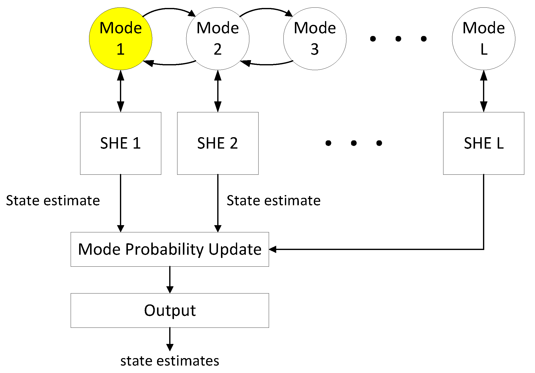
Based on the design of the single-state estimator in the previous section, this section will introduce the stochastic hybrid estimation algorithm [21] in this paper. The stochastic estimator algorithm is illustrated in Figure 4. To estimate the continuous and discrete states of WECSs, a robust estimator is used in this paper. The algorithm of a single robust estimator is given in Section 3.2. The discrete state estimated by the stochastic hybrid estimator is the state of the most likely previous state of the system, and the continuous state is the weighted sum of the outputs of the estimators. Since each estimator has been decoupled from the fault and the estimation error has been minimized, the entire stochastic hybrid estimator is not influenced by the fault input and the estimation is fairly accurate. State estimation of hybrid systems is quite complex. If the historical operating record of the hybrid system is not available, the possible evolutions of the hybrid system state may increase exponentially. In order to prevent this, a hybrid strategy similar to the interacting multiple model (IMM) algorithm is introduced to reduce the complexity of the algorithm from exponential to constant. The stochastic hybrid estimation algorithm is derived as follows:

Assume that the initial probability distribution of the mixed state $\left(w,x\right)$ is

$$p\left[x\left(0\right)|w\left(0\right)=i\right]=N_n\left(x\left(0\right);{\widehat{x}}_i\left(0\right),P_i\left(0\right)\right)$$

(37)

$$Pr\left\{w\left(0\right)=i\right\}={\alpha }_i\left(0\right)$$

(38)

where ${\alpha }_i\ge 0\left(\forall i\right),{\displaystyle \sum }_{i=1}^{n_d}{\alpha }_i\left(0\right)=1$. $p[\cdot ]$ is the discrete probability distribution, $Pr\{\cdot \}$ indicates the probability of an event. For state $i\in W:p\left[x\left(k\right)|w\left(k\right)=i,y\left(k\right)\right]=N_n\left(x\left(k\right);{\widehat{x}}_i\left(k\right),P_i\left(k\right)\right)$, the probability density distribution $p[w\left(k\right)|y\left(k\right)]$ of the state $i$ is calculated in real time.

The online running process in Figure 4 are shown as follows:

• Calculate the mixing probability: the mixing probability is defined as $Pr\left\{w\left(k\right)=i|w\left(k+1\right)=j,y\left(k\right)\right\},\left(i,j\in W\right)$. According to the Bayesian theory

  $$\begin{array}{l}Pr\left\{w\left(k\right)=i|w\left(k+1\right)=j,y\left(k\right)\right\}\\ =\frac{1}{C_j}Pr\{w\left(k+1\right)=j|w\left(k\right)=i,y\left(k\right)\}Pr\{w\left(k\right)|y\left(k\right)\}\end{array}$$

  (39)

  where

  $$C_j={\displaystyle \sum }_{i=1}^{n_d}Pr\left\{w\left(k+1\right)=j|w\left(k\right)=i,y\left(k\right)\right\}p[w\left(k\right)|y\left(k\right)]$$

  (40)

  is a constant. In order to calculate the Equation (39), the following method can be used to evaluate the state transition probability $p_{ij}=Pr\left\{w\left(k+1\right)=j|w\left(k\right)=i,y\left(k\right)\right\}$:
  For Markov jump systems, such as the Markov jump linear system of wind turbines established in Section 2, the Markov transition matrix has recorded the transition probability between states. Then $Pr\left\{w\left(k+1\right)=j|w\left(k\right)=i,y\left(k\right)\right\}$ in (39) can be written as:

  $$Pr\left\{w\left(k+1\right)=j|w\left(k\right)=i,y\left(k\right)\right\}=p_{ij}=const$$

  (41)
• Calculate the initial conditions of each robust estimator: at each moment, the initial state of each robust estimator can be approximated by a simple Gaussian distribution. The initial state (estimated mean ${\widehat{x}}_{j0}\left(k\right)$) of the $j$-th robust estimator can be given by:

  $${\widehat{x}}_{j0}\left(k\right)={\displaystyle \sum }_{i=1}^{n_d}Pr\left\{w\left(k\right)=i|w\left(k+1\right)=j,y\left(k\right)\right\}{\widehat{x}}_i\left(k\right)$$

  (42)
• Mode-matched filter: For each robust estimator, the estimated mean ${\widehat{x}}_j\left(k+1\right)$ is calculated under the current system condition $w\left(k\right)=j$. According to the calculation process of a single robust estimator in Section 3.2, the gain $L_j\left(w\left(k\right)\right)$ can be given by (27); the robust estimator (REs) can be given by (20), and the robust estimator residuals $r_j\left(k+1\right)$, weighting matrix $T_j\left(w\left(k+1\right)\right)$, and covariance matrix $S_j\left(w\left(k+1\right)\right)$ will be updated in a similar way.
• Update the discrete state probability density function: For each SHE, the likelihood function $p\left[y\left(k+1\right)|w\left(k+1\right)=j,y\left(k\right)\right]$ is

  $$\begin{array}{ll}{\Lambda }_j\left(k+1\right)& :=p\left[y\left(k+1\right)|w\left(k+1\right)=j,y\left(k\right)\right]\\ & =\mathcal{N}\left(r_j\left(k+1\right);0,S_j\left(w\left(k+1\right)\right)\right)\end{array}$$

  (43)

  where $r_j\left(k+1\right)$ and $S_j\left(w\left(k+1\right)\right)$ are the residual vectors and its covariance generated by the $j$-th robust estimator. By the Bayes’ theorem, the discrete state probability ${\alpha }_j\left(k+1|k+1\right):=Pr\left\{w\left(k+1\right)=j|y\left(k+1\right)\right\}$ is given by

  $${\alpha }_j\left(k+1|k+1\right)=\frac{1}{\delta }{\Lambda }_j\left(k+1\right)C_j$$

  (44)

  where $\delta$ is an appropriate normalizing constant.
• Output: the estimation of the continuous state is obtained by a weighted sum of the output of each robust estimator.

  $$\widehat{x}\left(k+1\right)={\displaystyle \sum }_{j=1}^{n_d}{\widehat{x}}_j\left(k+1\right){\alpha }_j\left(k+1|k+1\right)$$

  (45)
  The discrete state estimation is given by the discrete state with the highest probability.

  $$Pr\left\{w\left(k+1\right)=j|y\left(k+1\right)\right\}={\alpha }_j\left(k+1|k+1\right)$$

  (46)

  and

  $$\widehat{w}\left(k+1\right)=\begin{array}{c}argmax\\ j\end{array}Pr\left\{w\left(k+1\right)=j|y\left(k+1\right)\right\}$$

  (47)

4. Comprehensive Fault Detection and Isolation Method

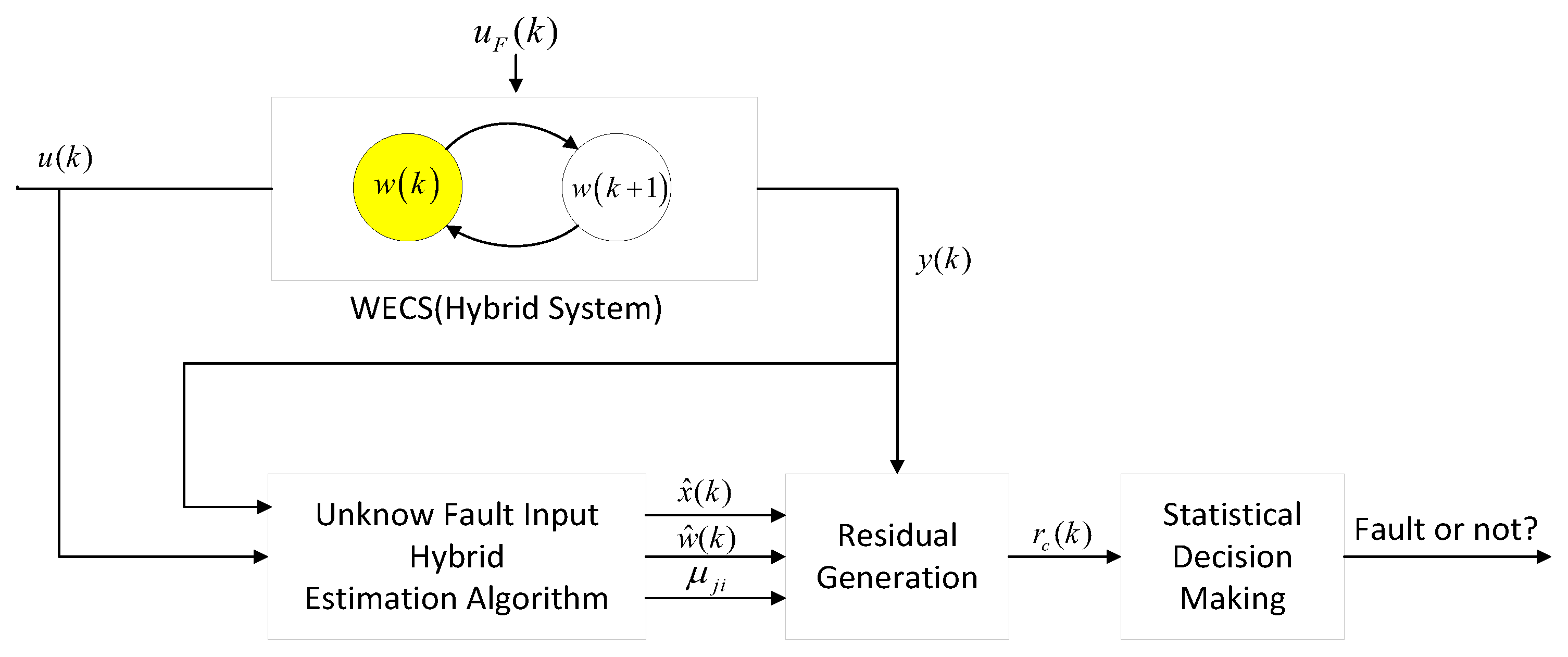
This section designs the FDI algorithm [21] for WECSs. Based on the results of Section 3, the state-space equation of the system is reconstructed by the idea of replication. Then, use the residual $r_c\left(k\right)$ to fit the fault input $u_F\left(k-1\right)$ of the system. Finally, statistical decision tools are used to determine whether the fitted fault input $u_F\left(k-1\right)$ is a fault. The block diagram of the FDI scheme is shown in Figure 5.

4.1. Residual Generation Algorithm and Reconstruction of the Fault

Before studying the characteristics of the residual, review the Assumption 2 of Section 2.3: the column rank of $F\left(w\left(k\right)\right)$ does not exceed the row rank of $C$. This assumption can be explained as to isolate different fault inputs, at least one of the elements corresponds to a single fault input in $r_c\left(k\right)$. $r_c\left(k\right)$ can be defined as:

$$\begin{array}{ll}{r}_c\left(k\right):=& W\left(k\right){\displaystyle {\displaystyle \sum }_{j=1}^{n_d}}{\alpha }_j(k|k-1)[\widehat{y}\left(k\right)-C(A_j{\widehat{x}}_j\left(k-1\right)+B_{j}u\left(k-1\right)\\ & +D\left(w\left(k-1\right)\right)+Iw\times yr\left(k-1\right))\end{array}$$

(48)

where

$$W\left(k\right)={[{\displaystyle \sum }_{j=1}^{n_d}{\alpha }_j(k|k-1)C{F}_j]}^{+}$$

(49)

$$\begin{array}{ll}{\alpha }_j\left(k|k-1\right)& :=Pr\left\{w\left(k\right)=j,y\left(k-1\right)\right\}\\ & ={\displaystyle {\displaystyle \sum }_{i=1}^{n_d}}Pr\left\{w\left(k\right)=j|w\left(k-1\right)=i,y\left(k-1\right)\right\}\\ & \times Pr\left\{w\left(k-1\right)=i,y\left(k-1\right)\right\}\\ & ={\displaystyle {\displaystyle \sum }_{i=1}^{n_d}}{\mu }_{ji}\left(k-1\right)Pr\left\{w\left(k-1\right)=i,y\left(k-1\right)\right\}\end{array}$$

(50)

where ${\mu }_{ji}=Pr\{w\left(k+1\right)=j|w\left(k\right)=i,y\left(k\right)\}$. To ensure that the algorithm proposed in this paper is solvable, make the following assumptions:

Assumption 3.

The Moore–Penrose pseudo-inverse solution of${{\displaystyle \sum }}_{j=1}^{n_d}{\alpha }_j(k|k-1)C{F}_j$.

Remark 1.

It is assumed by Assumption 2 that $C{F}_j$ is of full column rank. Therefore, only ${\alpha }_j(k|k-1)$ is distinct; let ${\displaystyle \sum }_{j=1}^{n_d}{\alpha }_j(k|k-1)$ be irreversible. Since ${\alpha }_j(k|k-1)$ is a random variable in the range $\left(0,1\right)$, it is almost inevitable that ${\alpha }_j(k|k-1$ takes the value of 0 at some specific time. ${{\displaystyle \sum }}_{j=1}^{n_d}{\alpha }_j\left(k|k-1\right)=1$, and $C{F}_j\ne 0$ make the ${{\displaystyle \sum }}_{j=1}^{n_d}{\alpha }_j(k|k-1)C{F}_j$ Moore–Penrose pseudo-inverse be able to be resolved.

Equation (48) gives to the residual $r_c\left(k\right)$ and output estimate $\widehat{y}\left(k\right)$ a one-to-one corresponding value. The following will demonstrate that the unknown fault inputs of the system can be estimated by $E[r_c\left(k\right)|\widehat{y}\left(k-1\right)]$.

Theorem 2.

Calculated from (48)–(50),$r_c\left(k\right)$ satisfies

$$E\left[r_c\left(k\right)|\widehat{y}\left(k-1\right)\right]=u_F\left(k-1\right)$$

(51)

$$r_c\left(k\right)~\mathcal{N}\left(u_F\left(k-1\right),\sigma \right)$$

(52)

where $\sigma >0$.

Proof. 

Based on the stochastic hybrid estimator in Section 3, coupled with the idea of replication, we can reconstruct the WECS system, and then use the reconstructed system to derive the unknown fault inputs.

Considering that the estimator designed in Section 3 is not affected by the actuator failure, we always have the relation $x\left(k\right)=\widehat{x}\left(k\right)$. Recalling (12), we obtain

$$\begin{array}{ll}\widehat{x}\left(k+1\right)& =A\left(w\left(k\right)\right)\widehat{x}\left(k\right)+B\left(w\left(k\right)\right)u\left(k\right)+F\left(w\left(k\right)\right)u_F\left(k\right)\\ & +D\left(w\left(k\right)\right)+D1\left(w\left(k\right)\right)e\left(k\right)+Iw\times yr\left(k\right)\end{array}$$

(53)

$$\begin{array}{ll}C\widehat{x}\left(k\right)=& C[A\left(w\left(k-1\right)\right)\widehat{x}\left(k-1\right)+B\left(w\left(k-1\right)\right)u\left(k-1\right)+F\left(w\left(k-1\right)\right)u_F\left(k-1\right)\\ & +D\left(w\left(k-1\right)\right)+D1\left(w\left(k-1\right)\right)e\left(k-1\right)+Iw\times yr\left(k-1\right)]\end{array}$$

(54)

$$\begin{array}{l}\widehat{y}\left(k\right)-C\left[A\left(w\left(k-1\right)\right)\widehat{x}\left(k-1\right)+B\left(w\left(k-1\right)\right)u\left(k-1\right)+D\left(w\left(k-1\right)\right)+Iw\times yr\left(k-1\right)\right]\\ =C\left[F\left(w\left(k-1\right)\right)u_F\left(k-1\right)+D1\left(w\left(k-1\right)\right)e\left(k-1\right)\right]\end{array}$$

(55)

Substituting (55) into (48), then

$$\begin{array}{ll}{r}_c\left(k\right)& =W\left(k\right){\displaystyle {\displaystyle \sum }_{j=1}^{n_d}}{\alpha }_j\left(k|k-1\right)C[F\left(w\left(k-1\right)\right)u_F\left(k-1\right)\\ & +D1\left(w\left(k-1\right)\right)e\left(k-1\right)]\end{array}$$

(56)

Combined with (49), then (56) can be reorganized as

$$\begin{array}{ll}{r}_c\left(k\right)& ={\left(CF\right)}^{+}\left[CF\left(w\left(k-1\right)\right)u_F\left(k-1\right)+C\times D1\left(w\left(k-1\right)\right)e\left(k-1\right)\right]\\ & =u_F\left(k-1\right)+{\left(CF\right)}^{+}C\times D1\left(w\left(k-1\right)\right)e\left(k-1\right)\end{array}$$

(57)

∵ $\mathrm{e}~\mathcal{N}\left(0,1\right)$, ∴

$$\begin{array}{ll}E\left[r_c\left(k\right)\right]& =E\left[u_F\left(k-1\right)+{\left(CF\right)}^{+}C\times D1\left(w\left(k-1\right)\right)e\left(k-1\right)\right]\\ & =u_F\left(k-1\right)+E\left[{\left(CF\right)}^{+}C\times D1\left(w\left(k-1\right)\right)e\left(k-1\right)\right]\\ & =u_F\left(k-1\right)\end{array}$$

(58)

Then (51) is proved. ☐

It is noted in (57) that the $r_c\left(k\right)$ and $e\left(k-1\right)$ are both satisfied with a Gaussian distribution, and letting $\sigma$, the variance of ${\left(CF\right)}^{+}C\times D1\left(w\left(k-1\right)\right)e\left(k-1\right)$, be a positive real number, then (52) is proved.

4.2. Statistical Decision-Making Algorithm

After calculating the residuals in Section 4.1, this section will design the FDI algorithm to detect any significant changes in the residuals which indicate faults. Section 4.1 showed that the residual follows a Gaussian distribution, and once the mean $r_c\left(k\right)$ is offset by 0, the system fails. There are many algorithms that can detect changes in time series. The algorithm for determining whether the system has failed is the same one to determine whether the mean value of the system fault input is 0. In this way, the purpose of fault isolation is achieved.

For the sake of determining each fault component separately, (52) is re-expressed as:

$$r_{c\left(i\right)}\left(k\right)~\mathcal{N}\left(u_{F\left(i\right)}\left(k-1\right),{\sigma }_i\right)$$

(59)

In order to detect significant changes in the system (deviation from mean value 0), a detection algorithm proposed by Segen [38] can be used. This algorithm can detect whether the random sequence is offset by the Gaussian process.

Define:

$${\xi }_i\left(k\right):=\frac{1}{\sqrt{2}}\left[{\displaystyle \sum }_{j=1}^k{r}_{c\left(i\right)}\left(j\right){\sigma }_i^{-1}{r}_{c\left(i\right)}\left(j\right)-1\right]$$

(60)

When the system state maintains a Gaussian random process, ${\xi }_i\left(k\right)$ is basically constant. When the system state deviates from the Gaussian process, ${\xi }_i\left(k\right)$ is a monotonic increasing function. Therefore, the difference $\Delta {\xi }_i\left(k\right)$ for ${\xi }_i\left(k\right)$, $\Delta {\xi }_i\left(k\right)$ is close to 0 when the system is in the Gaussian process. In contrary, when the system deviates from the Gaussian process ($\Delta {\xi }_i\left(k\right)>{\tau }_i^{*}$, ${\tau }_i^{*}$ is the set threshold), it can be determined that the input component has failed. The process to detect the fault input $u_F\left(k-1\right)$ and quantify its amount was shown in Algorithm 1.

Algorithm 1 The process to detect the fault input $u_F\left(k-1\right)$ and quantify its amount

For k = 1:T        % T is the simulation time   If $\Delta {\xi }_i\left(k\right)<{\tau }_i^{*}$ then    The system is normal;    $u_{F\left(i\right)}\left(k-1\right)=0$; % $u_{F\left(i\right)}\left(k-1\right)$ is the $i$-th component of fault input $u_F\left(k-1\right)$   Else    The system is abnormal;    $u_{F\left(i\right)}\left(k-1\right)=E\left[r_{c\left(i\right)}\left(k\right)|\widehat{y}\left(k-1\right)\right]$;   End If End For

5. Simulation Results

The simulations are designed and given in this chapter to validate the control effectiveness of the scenario-based SPMC controller, the performance of the stochastic hybrid estimator, and the fault detection and isolation ability of the proposed FDI algorithm.

Table 1. Model parameters.

Parameter	Value	Unit	Parameter	Value	Unit
$J_r$	90,000	$\mathrm{kg}\cdot {\mathrm{m}}^2$	$P_{g,nom}$	225	kW
$J_g$	10	$\mathrm{kg}\cdot {\mathrm{m}}^2$	${\omega }_{r,nom}$	4.29	rad/s
$K_s$	8 × 106	Nm/rad	${\omega }_{g,nom}$	105.534	rad/s
$D_s$	8 × 104	$\mathrm{kg}\cdot {\mathrm{m}}^2/\left(\mathrm{rad}\cdot \mathrm{s}\right)$	${\omega }_{r,min}$	3.5	rad/s
$N_g$	24.6	-	${\omega }_{g,min}$	86.1	rad/s
$ℛ$	14.5	m	${\theta }_{min}$	0	deg
${\tau }_{\theta }$	0.15	s	${\theta }_{max}$	25	deg
${\tau }_{\Gamma }$	0.1	s	${\left|\dot{\theta }\right|}_{max}$	10	deg/s

gives the physical parameters of the simulated WECS, which is a 225 kW power system [32]. As a prerequisite, the WECS model (4) is discretized and linearized to model (11) at three operating points (the wind speeds are 5, 8 and 11 m/s, respectively), and the parameters of the model are shown in

Table 2. Parameters of the linearized wind energy conversion system (WECS) model in different operation points.

$\mathit{v}\mathbf{\left(}\mathbf{m}\mathbf{/}\mathbf{s}\mathbf{\right)}$	Parameters
	a84	a88	e81	a1	a2	a3
$v_1=5$	−0.409	−0.50	1.90	0.3125	2.92	0.9375
$v_2=8$	−0.479	−0.53	2.31	0.33	3.65	2.3
$v_3=11$	−0.833	−0.53	2.50	0.625	5	5

.

With the WECS assembly model, the next step is to obtain the Markov transition matrix. Respectively, the input and state constraint are $T_g\in \left(-6000\mathrm{Nm},0\mathrm{Nm}\right)$ and $\beta \in \left(0^{°},{90}^{°}\right)$, prediction horizon $N=4$, scenario tree layer $n_{max}=3$, the Markov transition matrix $P=\left[\begin{array}{ccc}0.7230& 0.2770& 0\\ 0.1554& 0.8383& 0.0063\\ 0& 0.4138& 0.5862\end{array}\right]$, weight matrix $Q={\left[\begin{array}{cc}\begin{array}{cc}0& \cdots \\ ⋮& \ddots \end{array}& \begin{array}{ccc}0& 0& 0\\ ⋮& ⋮& ⋮\end{array}\\ \begin{array}{cc}0& \cdots \\ 0& \cdots \\ 0& \cdots \end{array}& \begin{array}{ccc}0& 0& 0\\ 0& 1& 0\\ 0& 0& 1\end{array}\end{array}\right]}_{9\times 9}$ and $R=\left[\begin{array}{cc}1& 0\\ 0& 1\end{array}\right]$.

Furthermore, the simulations are performed in the environment (MATLAB R2015a) on an Intel^® Core™ i5-2400 CPU 3.10 GHz RAM 4 GB (FOUNDER, Beijing, China). The simulation Simulink structure of the proposed FDI algorithm is shown in Figure 5, which contains three part: SMPC, SHE and FDI running synchronously. The major calculation load is solving a SMPC problem (14) quadratic constrained quadratic programming (QCQP), which costs 2.1 ms on average.

5.1. The Control Performance of the SMPC Controller without Fault

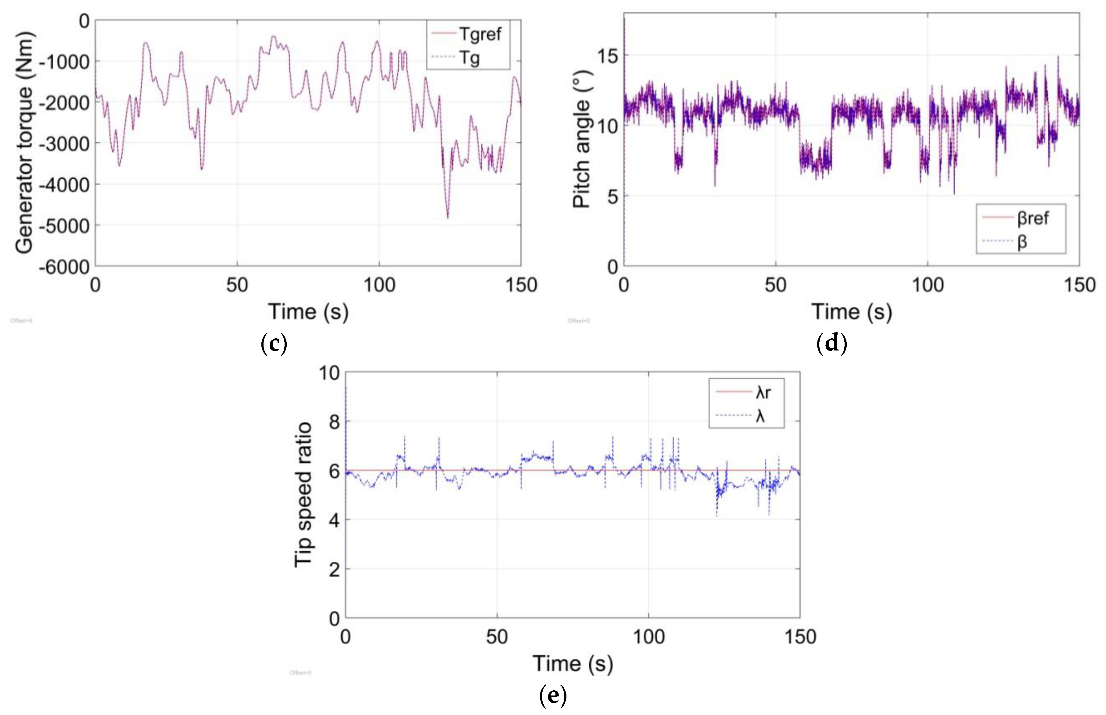
The control performance of the SMPC controller is investigated for a WECS without fault. In this simulation, the maximum power reference $P_{gref}$ can be given through reference to the table in [39]. Meanwhile, the generator speed reference ${\omega }_{gref}$ can be calculated with the best tip speed ratio $\lambda =6$. The Figure 6 shows the tracking performance of a wind energy conversion system’s maximum wind energy under the random wind speed. All the red solid and blue dotted lines are the WECS references and outputs, respectively. First, the tracking of maximum power and generator speed are shown in Figure 6a,b. It can be seen that the proposed SMPC controller has good control performance to minimize the tracking errors. Meanwhile, Figure 6d reveals that there has been a steady fluctuation for the pitch angle $\beta$ (about 7–12°) in accordance with the actual situation. Finally, as shown in Figure 6e, the tip speed ratio $\lambda$ is close to its optimal value ${\lambda }_{opt}=6$ with limited tracking errors. These simulation results indicate that in normal status, the presented stochastic model predictive controller can capture the maximum wind energy precisely and effectively.

5.2. Stochastic Hybrid Estimation with Unknown Fault Inputs

In this section, the simulations are designed and implemented to verify the effectiveness of the proposed stochastic hybrid estimator with unknown fault inputs.

First, the pre-defined faults are shown in Figure 7a. The faults of the generator torque reference $T_{gref}$ occur at $\left(100,130\mathrm{s}\right)$, and the fault values are from 0 to 500 Nm; the time range of the input fault pitch angle reference ${\beta }_{ref}$ is $\left(110,140\mathrm{s}\right)$ and the pitch angle values are in the range (0–6°). This setting of the faults is based on two purposes: (1) the set of the time range can investigate different combinations of the two kinds of actuators’ faults (only $T_{gref}$ failure in $\left(100,110\mathrm{s}\right)$, $T_{gref}$ failure and ${\beta }_{ref}$ failure at the same time in $\left(110,130\mathrm{s}\right)$, and only ${\beta }_{ref}$ failure in $\left(130,140\mathrm{s}\right)$); (2) the set of the value range can cover all three operating domains of the WECS. Therefore, the fault sets are reasonable to verify the estimation performance of the proposed stochastic hybrid estimator.

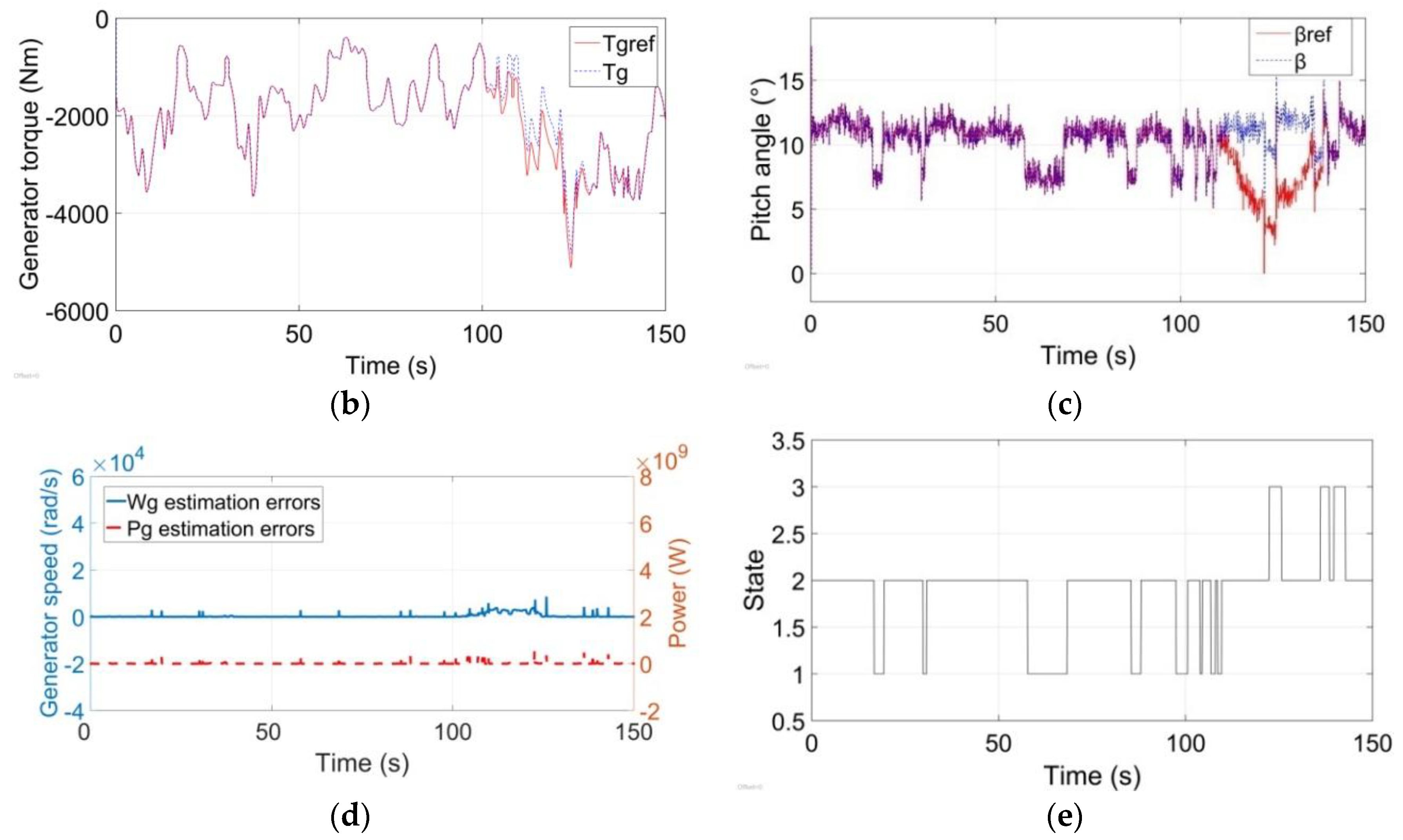
Second, Figure 7b,c show the bad tracking performance of the actuators caused by the fault set above. In the period of $\left(100,130\mathrm{s}\right)$ in Figure 7b, the generator torque $T_g$ cannot achieve the set value $T_{gref}$ when the actuator is faulty. Meanwhile, the pitch angle reference ${\beta }_{ref}$ in Figure 7c has obvious errors when the fault occurs from 110 s to 140 s. These results suggest that the actuators’ fault cannot be ignored since it leads to bad operating performance of the WECS.

Third, the proposed stochastic hybrid estimator is used to estimate the system states (including the discrete states and the continuous states). Figure 7d shows the estimation results of the generator speed and the power of the WECS. The estimation errors are very small, this means the proposed estimator can estimate the states of the WECS effectively. Meanwhile, the estimation error has only small fluctuations during the simulation, which suggests the estimator has stable estimation performance. Figure 7e is the estimation of the discrete state of the WECS. Each discrete state represents one working point of the WECS. The proposed method can quickly and precisely estimate the current working point of the WECS. Notably, the proposed estimator does not have the information of the fault sets, this means the estimator is robust to the faults of the actuators. This is valuable for designing a fault detection algorithm to detect whether the WECS is in fault mode, which is one optional future work for the authors.

5.3. Fault Detection and Isolation of WECS

In this section, the simulation is given to verify the comprehensive FDI algorithm to accomplish the fault diagnosis and isolation of a WECS with an unknown actuator fault input. This section follows the same fault sets in Section 5.2. Figure 8a shows the unknown fault inputs residuals, which are generated by the proposed FDI algorithm. The time of the fitted fault by the FDI algorithm is the same as the time of the pre-defined fault, and the value of the fitted fault is in the small range around the fault. Besides, it can be seen that the $T_{gref}$ fluctuation is smaller and the pitch angle reference ${\beta }_{ref}$ fluctuation is relatively larger. This is because the amplitude of the $T_{gref}$ is about 1000 times larger than the value of ${\beta }_{ref}$. Therefore, the impact of the Gaussian white noise on $T_{gref}$ is very small. The simulation results show that the proposed FDI algorithm can fit the fault input accurately.

Figure 8b is the result of the statistical decision part of the FDI method. This decision is based on the quantitatively fitting results in the Figure 8a. To make the decision, we set a small threshold ${\tau }_i^{*}$ (such as 0.05) to the statistical decision result in Figure 8b. When the curve indicating the probability of failure of $T_{gref}$ and ${\beta }_{ref}$ exceeds the threshold, it is determined that the WECS has faults. Figure 8b precisely indicates that the $T_{gref}$ has failed in the time range $\left(100,130\mathrm{s}\right)$, and ${\beta }_{ref}$ has failed in that of $\left(110,140\mathrm{s}\right)$. The determination result is in accordance with the fault sets of Figure 7a, and the determination results of the two failures do not affect each other. These results suggest that the fault diagnosis and isolation are all achieved with great success.

6. Conclusions

This paper proposes a comprehensive stochastic hybrid state estimation and FDI method for WECSs. To describe the stochastic dynamics of the WECS, the Markov-jump linear model is developed. Based on this model, the SMPC controller with a scenario-tree gives good control performance of the WECS. With the closed-loop control system, the stochastic hybrid estimation is studied and used to estimate the system states. Finally, based on the information from the proposed estimator, the FDI algorithm is given to implement the fault detection and isolation of the WECS’ actuators unknown fault inputs. The simulation results suggest that the proposed method has good FDI performance, and that is a powerful method for the fault detection and isolation of WECS.

However, this work only considers the unknown fault inputs $u_F\left(k\right)$. Future research should be undertaken to investigate other uncertainties (such as parametric variations, faults on the outputs measurements, etc.). Furthermore, the proposed stochastic hybrid estimation and FDI algorithm may be integrated to mitigate voltage dips [2,3] to improve the industrial value of the proposed method.

References

1. Nedaei, M.; Assareh, E.; Walsh, P.R. A comprehensive evaluation of the wind resource characteristics to investigate the short term penetration of regional wind power based on different probability statistical methods. Renew. Energy 2018, 128, 362–374. [Google Scholar] [CrossRef]
2. Morshed, M.J.; Fekih, A. A comparison study between two sliding mode based controls for voltage sag mitigation in grid connected wind turbines. In Proceedings of the 2015 IEEE Conference on Control Applications (CCA), Sydney, NSW, Australia, 21–23 September 2015; pp. 1913–1918. [Google Scholar]
3. Morshed, M.J.; Fekih, A. A new fault ride-through control for DFIG-based wind energy systems. Electr. Power Syst. Res. 2017, 146, 258–269. [Google Scholar] [CrossRef]
4. Shi, Y.T.; Kou, Q.; Sun, D.H.; Li, Z.X.; Qiao, S.J.; Hou, Y.J. H Fault Tolerant Control of WECS Based on the PWA Model. Energies 2014, 7, 1750–1769. [Google Scholar] [CrossRef]
5. Shi, Y.T.; Xiang, X.; Wang, L.; Zhang, Y.; Sun, D.H. Stochastic Model Predictive Fault Tolerant Control Based on Conditional Value at Risk for Wind Energy Conversion System. Energies 2018, 11, 193. [Google Scholar] [CrossRef]
6. Bernardini, D.; Bemporad, A. Stabilizing model predictive control of stochastic constrained linear systems. IEEE Trans. Autom. Control 2012, 57, 1468–1480. [Google Scholar] [CrossRef]
7. Sampathirao, A.K.; Sopasakis, P.; Bemporad, A.; Patrinos, P.P. GPU-Accelerated Stochastic Predictive Control of Drinking Water Networks. IEEE Trans. Control Syst. Technol. 2018, 26, 551–562. [Google Scholar] [CrossRef] [Green Version]
8. Zhang, Y.; Meng, F.; Wang, R.; Zhu, W.; Zeng, X.-J. A stochastic MPC based approach to integrated energy management in microgrids. Sustain. Cities Soc. 2018, 41, 349–362. [Google Scholar] [CrossRef]
9. Cominesi, S.R.; Farina, M.; Giulioni, L.; Picasso, B.; Scattolini, R. A Two-Layer Stochastic Model Predictive Control Scheme for Microgrids. IEEE Trans. Control Syst. Technol. 2018, 26, 1–13. [Google Scholar] [CrossRef]
10. Zhang, Q.; Deng, W.; Li, G. Stochastic Control of Predictive Power Management for Battery/Supercapacitor Hybrid Energy Storage Systems of Electric Vehicles. IEEE Trans. Ind. Inf. 2018, 14, 3023–3030. [Google Scholar] [CrossRef]
11. Moser, D.; Schmied, R.; Waschl, H.; del Re, L. Flexible Spacing Adaptive Cruise Control Using Stochastic Model Predictive Control. IEEE Trans. Control Syst. Technol. 2017, 26, 114–127. [Google Scholar] [CrossRef]
12. Parisio, A.; Rikos, E.; Glielmo, L. Stochastic model predictive control for economic/environmental operation management of microgrids: An experimental case study. J. Process Control 2016, 43, 24–37. [Google Scholar] [CrossRef] [Green Version]
13. Baloch, M.H.; Wang, J.; Kaloi, G.S. A review of the state of the art control techniques for wind energy conversion system. Int. J. Renew. Energy Res. 2016, 6, 1277–1295. [Google Scholar]
14. Ćetenović, D.N.; Ranković, A.M. Optimal parameterization of Kalman filter based three-phase dynamic state estimator for active distribution networks. Int. J. Electr. Power Energy Syst. 2018, 101, 472–481. [Google Scholar] [CrossRef]
15. Crisan, D.; Míguez, J. Nested particle filters for online parameter estimation in discrete-time state-space Markov models. Bernoulli 2018, 24, 3039–3086. [Google Scholar] [CrossRef]
16. Hu, Y.-W.; Zhang, H.-C.; Liu, S.J.; Lu, H.T. Sequential Monte Carlo Method toward Online RUL Assessment with Applications. Chin. J. Mech. Eng. 2018, 31. [Google Scholar] [CrossRef]
17. Pradeep, C.; Cao, Y.; Murugesu, R.; Rakkiyappan, R. An event-triggered synchronization of semi-Markov jump neural networks with time-varying delays based on generalized free-weighting-matrix approach. Math. Comput. Simul. 2017. [Google Scholar] [CrossRef]
18. Li, L.; Qi, W.; Chen, X.; Kao, Y.; Gao, X.; Wei, Y. Stability analysis and control synthesis for positive semi-Markov jump systems with time-varying delay. Appl. Math. Comput. 2018, 332, 363–375. [Google Scholar] [CrossRef]
19. Rakkiyappan, R.; Maheswari, K.; Velmurugan, G.; Park, J.H. Event-triggered Hinfinity state estimation for semi-Markov jumping discrete-time neural networks with quantization. Neural Netw. 2018, 105, 236–248. [Google Scholar] [CrossRef] [PubMed]
20. Rakkiyappan, R.; Maheswari, K.; Sivaranjani, K.; Joo, Y.H. Non-fragile finite-time l2l state estimation for discrete-time neural networks with semi-Markovian switching and random sensor delays based on Abel lemma approach. Nonlinear Anal. Hybrid Syst. 2018, 29, 283–302. [Google Scholar] [CrossRef]
21. Liu, W.; Hwang, I. Robust estimation and fault detection and isolation algorithms for stochastic linear hybrid systems with unknown fault input. IET Control Theory Appl. 2011, 5, 1353–1368. [Google Scholar] [CrossRef]
22. Beddek, K.; Merabet, A.; Kesraoui, M.; Tanvir, A.A.; Beguenane, R. Signal-Based Sensor Fault Detection and Isolation for PMSG in Wind Energy Conversion Systems. IEEE Trans. Instrum. Meas. 2017, 66, 2403–2412. [Google Scholar] [CrossRef]
23. Simani, S.; Farsoni, S.; Castaldi, P. Fault Diagnosis of a Wind Turbine Benchmark via Identified Fuzzy Models. IEEE Trans. Ind. Electron. 2015, 62, 3775–3782. [Google Scholar] [CrossRef]
24. Bessa, I.V.D.; Palhares, R.M.; Filho, J.E.C. Data-driven fault detection and isolation scheme for a wind turbine benchmark. Renew. Energy 2016, 87, 634–645. [Google Scholar] [CrossRef]
25. Dey, S.; Pisu, P.; Ayalew, B. A Comparative Study of Three Fault Diagnosis Schemes for Wind Turbines. IEEE Trans. Control Syst. Technol. 2015, 23, 1853–1868. [Google Scholar] [CrossRef]
26. Badoud, A.E.; Khemliche, M.; Bouamama, B.O.; Bacha, S. Bond Graph Algorithms for Fault Detection and Isolation in Wind Energy Conversion. Arab. J. Sci. Eng. 2014, 39, 4057–4076. [Google Scholar] [CrossRef]
27. Fernandez-Canti, R.M.; Blesa, J.; Tornil-Sin, S.; Puig, V. Fault detection and isolation for a wind turbine benchmark using a mixed Bayesian/Set-membership approach. Annu. Rev. Control 2015, 40, 59–69. [Google Scholar] [CrossRef] [Green Version]
28. Zhang, J.; Xiong, J.; Ren, M.; Shi, Y.; Xu, J. Filter-Based Fault Diagnosis of Wind Energy Conversion Systems Subject to Sensor Faults. J. Dyn. Syst. Meas. Control 2016, 138, 061008. [Google Scholar] [CrossRef]
29. Peng, Y.; Qiao, W.; Qu, L.; Wang, J. Sensor fault detection and isolation for a wireless sensor network-based remote wind turbine condition monitoring system. In Proceedings of the IEEE Industry Applications Society Meeting, Cincinnati, OH, USA, 1–5 October 2017. [Google Scholar]
30. Song, Z.; Geng, X.; Kusiak, A.; Xu, C. Mining Markov chain transition matrix from wind speed time series data. Expert Syst. Appl. 2011, 38, 10229–10239. [Google Scholar] [CrossRef]
31. Ross, S.M. Introduction to Probability Models, 1st ed.; Elsevier: New York, NY, USA, 2007. [Google Scholar]
32. Thomsen, S. Nonlinear Control of a Wind Turbine. Master’s Thesis, Technical University of Denmark, Kongens Lyngby, Denmark, 2006. [Google Scholar]
33. Slootweg, J.G.; Polinder, H.; Kling, W.L. Dynamic modeling of a wind turbine with doubly fed induction generator. In Proceedings of the 2001 Power Engineering Society Summer Meeting, Vancouver, BC, Canada, 15–19 July 2001; pp. 644–649. [Google Scholar]
34. Bryson, A.E. Applied Linear Optimal Control: Examples and Alogrithms; Cambridge University Press: Cambridge, UK, 2002. [Google Scholar]
35. Parlangeli, G.; Valcher, M.E. Optimal filtering, fault detection and isolation for linear discrete-time systems in a noisy environment. Int. J. Adapt. Control Signal Process. 2003, 17, 729–750. [Google Scholar] [CrossRef]
36. Chen, J.; Patton, R.J. Optimal filtering and robust fault diagnosis of stochastic systems with unknown disturbances. IEEE Proc. Control Theory Appl. 1996, 143, 31–36. [Google Scholar] [CrossRef]
37. Kitanidis, P.K. Unbiased minimum-variance linear state estimation. Automatica 1987, 23, 775–778. [Google Scholar] [CrossRef]
38. Segen, J.; Sanderson, A. Detecting Change in a Time-Series. IEEE Trans. Inf. Theory 1980, 26, 249–255. [Google Scholar] [CrossRef]
39. Munteanu, I. Optimal Control of Wind Energy Systems; Springer: Berlin, Germany, 2008. [Google Scholar]
Figure 1. Wind speed and the corresponding working point.
Energies 11 02227 g001
Figure 2. The structure of wind energy conversion system (WECS).
Energies 11 02227 g002
Figure 3. The trend of the power coefficient C p , the tip-speed ratio λ and the pitch angle β following the wind speed: (a) The power coefficient C p ( λ , β ) function; (b) Relationship between C p and β at the best tip speed ratio.
Energies 11 02227 g003
Figure 4. The proposed stochastic hybrid estimation (SHE) algorithm (where the yellow model just denote different model, model L represent that there is a lot of models.).
Energies 11 02227 g004
Figure 5. Structure of the proposed FDI (fault detection and isolation) algorithm (where the yellow model just denote different model).
Energies 11 02227 g005
Figure 6. Wind energy conversion system’s maximum wind energy capture under random wind speed with the stochastic model predictive controller: (a) maximum power capture; (b) generator speed ω g ; (c) generator torque T g r e f ; (d) input pitch angle β r e f ; (e) tip speed ratio.
Energies 11 02227 g006aEnergies 11 02227 g006b
Figure 7. The settings of the WECS actuator’s unknown fault inputs, the system continuous state estimation error and discrete state estimated by the stochastic hybrid estimator: (a) unknown fault inputs setting of the generator torque and pitch angle; (b) the input generator torque reference T g r e f ; (c) the input pitch angle reference β r e f ; (d) estimation error of output continuous state generator speed ω g and power P g ; (e) estimation of the WECS discrete states.
Energies 11 02227 g007aEnergies 11 02227 g007b
Figure 8. Fitting the WECS actuator unknown fault inputs, fault diagnosis and isolation results: (a) Fault residuals of the system unknown input generator torque reference T g r e f and pitch angle reference β r e f ; (b) Fault model probability.
Energies 11 02227 g008