High Efficiency and Power Tracking Method for Wireless Charging System Based on Phase-Shift Control

Abstract

The paper presents optimal operating point tracking algorithm for wireless charging system using identical coupling coils providing us to meet simultaneously high efficiency and high transmitted power under varied load and detuning conditions. The proposed method is suitable either for purely resistive load or battery load and it is based on phase-shift control between the primary and the secondary voltage. The paper also gives an intuitive mathematical description of the key control idea and demonstrates its operational abilities. The proposed algorithm is finally implemented into digital signal processor (DSP) and tested on 4 kW laboratory prototype of shielded wireless power transfer system.

1. Introduction

Over the past few years the modern industry has recorded a huge and intensive development that has brought many technical upgrades in public transportation leading in less energy consumption and improving environmental issues. The most frequently argued topic is the vision to replace the conventional combustion engine vehicles with electric vehicles (EVs), e.g., [1,2]. The initial concept of EV comes from the previous experience with hybrid electric vehicles (HEVs), which later evolved into the popular plug-in hybrid vehicles (PHEVs). In addition to their valuable environmental benefits, they also deal with several technical problems, such as the need for conductive (cable) charging and the relating requirements on galvanic insulation of on-board electronics. With this respect, many organizations are devoting considerable resources to research and development in the field of wireless power transfer (WPT) technologies. Such systems offer high charging comfort and safety, since they prevent any risk of electric shock when charging either in the rain or snow [3,4,5,6]. They possibly find their purpose in cooperation with intelligent systems of modern “smart” houses working as a bi-directional power storage [7,8].

Technical disadvantages, such as the efficiency influenced by many operational efficiency matters, long charging time, and strict hygiene constraints [9] slow down the mass expansion of WPT technologies on the market. To deal with these issues, an industry-wide specification guideline that defines acceptable criteria for interoperability, electromagnetic compatibility, minimum performance and efficiency, safety, and testing for wireless charging of light duty electric and plug-in EVs was developed by Society of Automotive Engineers International (SAE) and established in standard SAE TIR J2954 [10].

The available literature collects large number of complex studies addressing all particular issues relating to WPT systems. A considerable attention has been paid to the design optimization and the systems operational characteristics. An exhaustive theoretical discussion on this topic is given for example in [11,12,13,14,15,16,17,18,19,20,21,22,23,24,25,26,27,28,29,30,31,32]. The authors usually build their mathematical models based on the equivalent electrical circuit method using linear equations with lumped electrical parameters, but only few of them consider also the parasitic effects (e.g., [12,13,14,15,16]). Another frequently proposed approach is to describe the system behaviour while using electromagnetic field calculated through the finite element analysis [28,29,30,31,32,33,34,35,36,37,38,39,40]. A great effort has been devoted also to the control strategies [41,42,43,44,45,46,47,48].

In [41], the authors propose a concept that maximizes the efficiency and increases the amount of extractable power of the WPT system working with non-resonant coupling. The method is based on the adaption of the equivalent load impedance by settings a phase-shift between current and voltage in the active rectifier. A similar mechanism also using the active rectifier, which is additionally equipped with an auxiliary measurement coil, is proposed in [42]. The suggested algorithm can regulate separately both the equivalent load impedance and the output voltage while providing slight improvements in systems performance.

Another crucial solution is described in [43], but its major drawback is that the resistive and the reactive part of the load impedance cannot be controlled independently, and therefore the overlapping of maximum efficiency and transmitted power is not reached widely. Another effective method to maximise the operational efficiency is proposed in [44]. It uses matching the converter’s output frequency with the receiver’s self-resonant frequency. The method is suitable for WPT systems where the application requires the variable load, the changing mutual coil position, and the fluctuating environmental conditions. However, to the authors’ best knowledge, very few publications exist that should help with efficiency and power maximization across the specific range of load and coupling coils position. As shown in [49], fast charging of lithium-ion batteries is highly demanded to facilitate the use of electric vehicles. Therefore, the importance of overlapping high performance and efficiency is very actual.

This work introduces the operation point tracking algorithm that enables to simultaneously reach high efficiency and high transmitted power even for changing load and varying mutual position of coupling coils. The proposed method is applicable either for purely resistive load or battery load, and it is based on phase-shift control between the primary and the secondary voltage.

2. Analyses of Proposed Tracking Algorithm

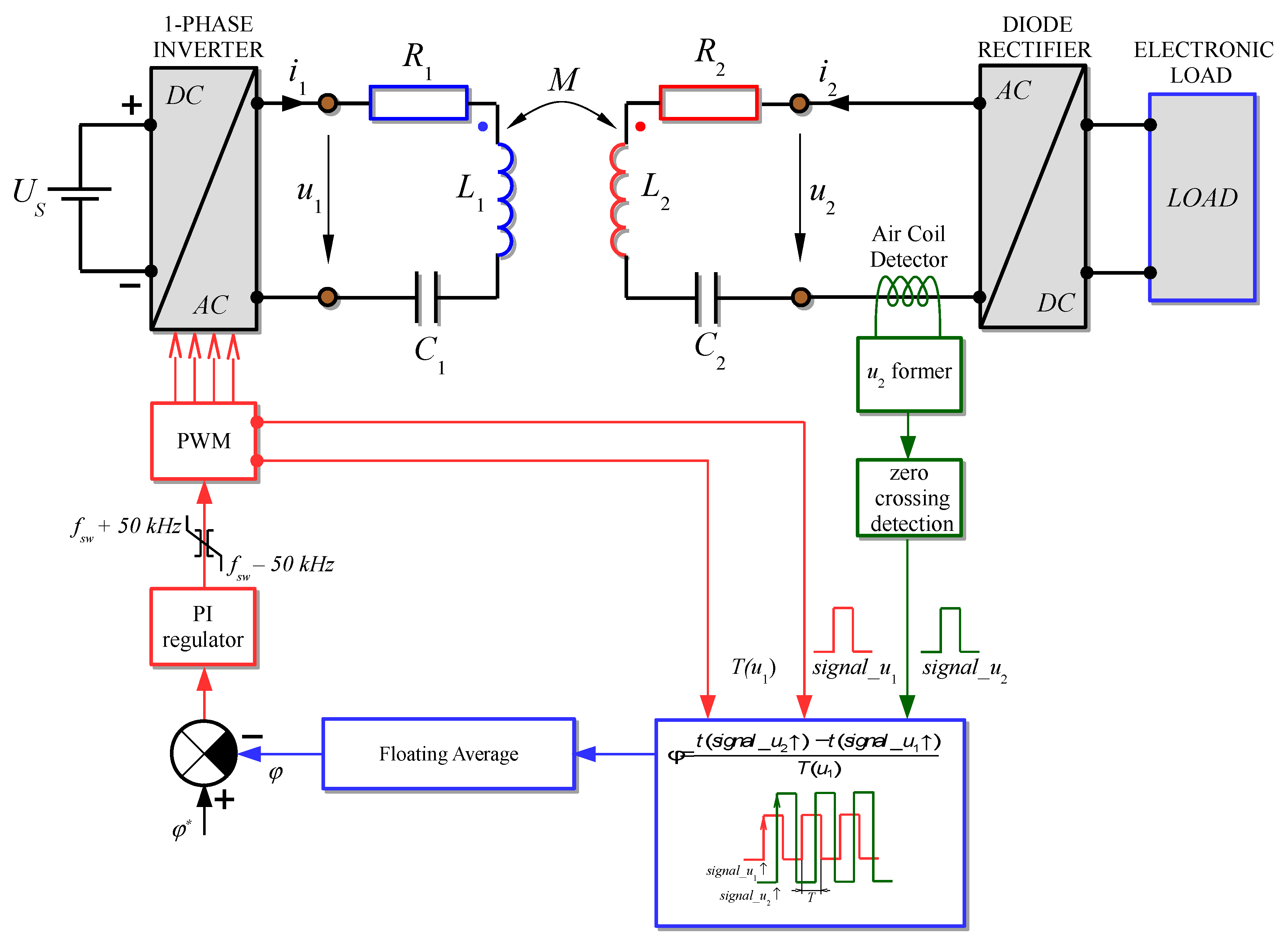
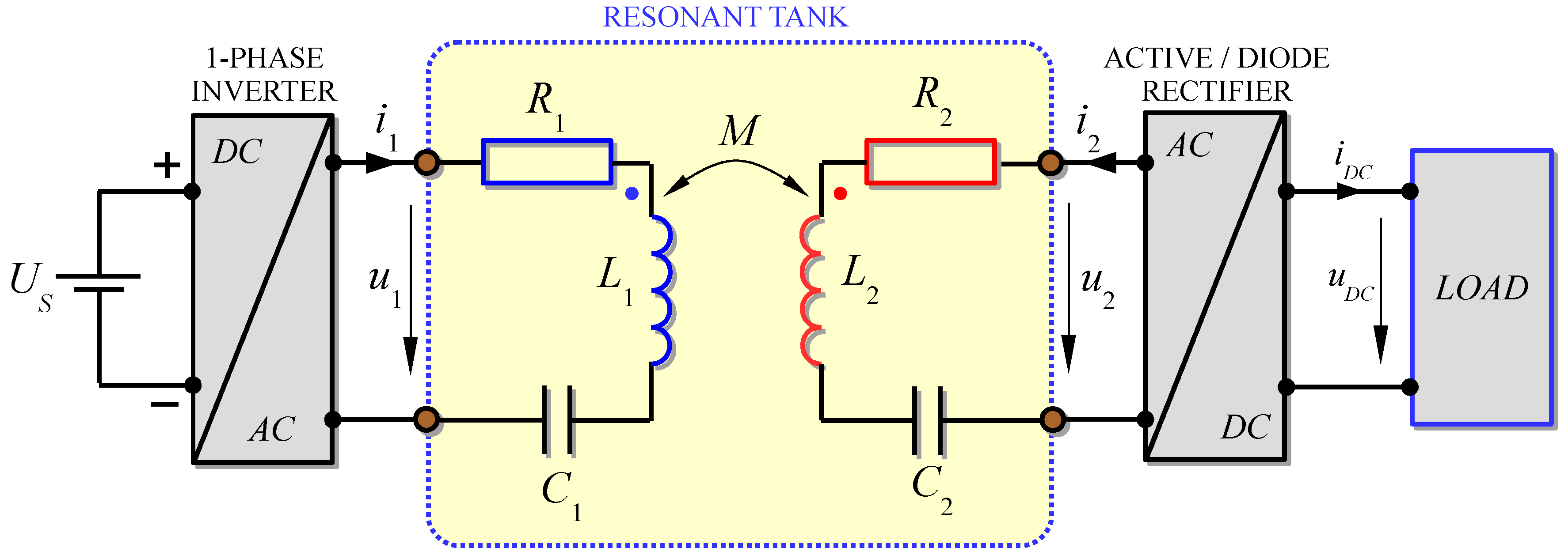
The basic idea of the proposed control method might be understood from Figure 1. The resonant tank uses a series-series compensation to gain the constant current acting output, which is the most suitable for charging EVs. The coupling coils are both modelled with an equivalent electrical circuit neglecting additional parasitic effects.

The parameters R₁ and R₂ represent the coils’ equivalent series resistances, L₁ and L₂ introduce the self-inductances, and M forms their mutual inductance. Compensation capacitors C₁ and C₂ are both of high quality and low ESR to meet high overall operational quality factor.

The system is supplied from a dc source U_S via single-phase (H-bridge) inverter controlling both legs with duty cycle of 50%. Thus, the inverter supplies the transmitting coil with square-wave voltage of amplitude U_S and zero average value. The load could be either the battery pack with a dc/dc voltage converter, or the resistive load. It depends on application and whether the active or diode rectifier at the secondary side is applied. The resonant circuit acts as a band-pass filter with relatively good frequency selectivity, and therefore, the first harmonic approximation may be used for the analyses. In the case of the active rectifier use, we can proceed, as follows. First, the fundamental harmonic component of terminal voltage u₁ and its RMS value U₁ are defined in Equation (1)

$$u_1=\frac{4}{\mathsf{\pi }}{U}_S\sin \left(\omega t\right), U_1=\frac{2\sqrt{2}}{\mathsf{\pi }}{U}_S.$$

(1)

According to the phase modulation angle, the secondary voltage u₂ may be expressed either as time-domain or phasor quantity

$$u_2=U_2\sin \left(\omega t-\varphi \right), \mathrm{and} {\overline{U}}_2=U_2\left[\cos \left(\varphi \right)+j\sin \left(\varphi \right)\right]$$

(2)

The phase shift φ varies depending on the overall load reactance character dominant at the working frequency. Secondly, based on equivalent circuit method and the symbolic complex expression, we describe the resonant tank using a set of two Equations (3).

$$\left[\begin{array}{c}{\overline{I}}_1\\ {\overline{I}}_2\end{array}\right]=\left[\begin{array}{cc}{R}_1+j\left(\omega L_1-\frac{1}{\omega C_1}\right)& -j\omega M\\ -j\omega M& R_2+j\left(\omega L_2-\frac{1}{\omega C_2}\right)\end{array}\right]\backslash \left[\begin{array}{c}{\overline{U}}_1\\ -{\overline{U}}_2\end{array}\right]$$

(3)

Here, the quantities ${\overline{U}}_1$, ${\overline{I}}_1$, and ${\overline{I}}_2$ symbolize, respectively, the phasor of the input voltage and primary and secondary currents. Moreover, when both coupling coils are identical, the model Equation (3) might be further simplified with assumption Equation (4).

$$R_1=R_2=R, L_1=L_2=L, C_1=C_2=C$$

(4)

While neglecting losses produced in both the voltage-source inverter and rectifier, we can easily derive the input and output power and system efficiency, as in Equation (5). Here, the symbol $“\ast ”$ represents the complex conjugate multiplication and $“R”$ is the real part of a complex number.

$$P_{IN}=\Re \left\{{\overline{U}}_1{\overline{I}}_1^{\ast }\right\}, P_{OUT}=\Re \left\{{\overline{U}}_2{\overline{I}}_2^{\ast }\right\} and \eta =\frac{\Re \left\{{\overline{U}}_2{\overline{I}}_2^{\ast }\right\}}{\Re \left\{{\overline{U}}_1{\overline{I}}_1^{\ast }\right\}}$$

(5)

As known, the resonant tank can electrically resonate at three different frequencies Equation (6). Generally, it depends both on the load and the mutual inductance whether the main f_sw01 or one of the sideband f_sw02,03 resonant frequencies will dominate.

$$f_{sw01}=\frac{1}{2\mathsf{\pi }\sqrt{LC}}, f_{sw02,03}=\frac{1}{2\mathsf{\pi }\sqrt{\left(L\pm M\right)C}}$$

(6)

For a given mutual inductance, the system resonates at f_sw01 when the equivalent load (derived from the secondary voltage and current) is larger than the optimal load Equation (7), referred, for example, in [2], and on the contrary, we can expect the sideband resonant frequency dominant when it is lower than the optimal load.

$$R_{opt}=\sqrt{R^2+M^2{\omega }^2}$$

(7)

Therefore, the solution must expand into two separated solutions. With assumption of operational state, where the equivalent load R_eq is higher than the optimal load Equation (8),

$$R_{eq}=\frac{u_{DC}}{i_{DC}}\gg \sqrt{R^2+M^2{\omega }^2}$$

(8)

we may calculate the secondary complex conjugated current, as Equation (9).

$${\overline{I}}_2^{\ast }=\frac{-U_{2}Rcos\left(\varphi \right)+j\left(U_{2}Rsin\left(\varphi \right)-\omega M{U}_1\right)}{M^2{\omega }^2+R^2}$$

(9)

According to Equation (5), the output power is further found from Equation (10).

$$\begin{gathered} P_{OUT}=\Re \left\{\frac{-U_{2}R\cos \left(\varphi \right)+j\left(U_{2}R\sin \left(\varphi \right)-\omega M{U}_1\right)}{M^2{\omega }^2+R^2}{U}_2\left[\cos \left(\varphi \right)+j\sin \left(\varphi \right)\right]\right\} \\ =\frac{-R U_2^2+M{U}_1{U}_2\omega \sin \left(\varphi \right)}{M^2{\omega }^2+R^2} \end{gathered}$$

(10)

The phase shift at which the system delivers maximum power to the load can be determined by the solution of Equation (11).

$$\frac{d}{d\varphi }\left(\frac{-R U_2^2+M{U}_1{U}_2\omega sin\left(\varphi \right)}{M^2{\omega }^2+R^2}\right)=0$$

(11)

A short derivation leads to Equation (12), which for the observed interval is fulfilled when $\varphi =\mathsf{\pi }/2$.

$$\frac{M\omega U_1{U}_{2}cos\left(\varphi \right)}{M^2{\omega }^2+R^2}=0$$

(12)

The second solution takes place when the system resonates at some of the side-band frequencies Equation (6). In that case, the secondary complex conjugated current is as follows.

$${\overline{I}}_2^{\ast }=\frac{-\omega M{U}_1-\left(\omega M-jR\right)U_{2}cos\left(\varphi \right)+\left(j\omega M+R\right)U_{2}sin\left(\varphi \right)}{2MR{\omega }^2-j{R}^2}$$

(13)

Hence, with consideration of Equation (5), the formula for calculation of the output power changes from Equation (10) into Equation (14).

$$\begin{gathered} P_{OUT} \\ =\Re \left\{\frac{-\omega M{U}_1-\left(\omega M-jR\right)U_2\cos \left(\varphi \right)+\left(j\omega M+R\right)U_2\sin \left(\varphi \right)}{2MR{\omega }^2-j{R}^2}{U}_2\left[\cos \left(\varphi \right) \\ +j\sin \left(\varphi \right)\right]\right\}=-U_2\frac{U_2\left(R^2+2M^2{\omega }^2\right)+M{U}_1\omega \left[2M\omega \cos \left(\varphi \right)-Rsin\left(\varphi \right)\right]}{R^3+4M^{2}R{\omega }^2} \end{gathered}$$

(14)

The phase shift at which the system delivers maximum power to the load can be determined by the solution of (15).

$$\frac{d}{d\varphi }\left(-U_2\frac{U_2\left(R^2+2M^2{\omega }^2\right)+M{U}_1\omega \left[2M\omega cos\left(\varphi \right)-Rsin\left(\varphi \right)\right]}{R^3+4M^{2}R{\omega }^2}\right)=0$$

(15)

After short manipulation, we get Equation (16), which for observed interval is fulfilled when $\varphi =\mathsf{\pi }$.

$$\frac{M\omega U_1{U}_2\left(R\cos \left(\varphi \right)+2M\omega \sin \left(\varphi \right)\right)}{R^3+4M^{2}R{\omega }^2}=0$$

(16)

The system can never natively reach the operational point at which the maximum of efficiency absolutely overlaps the maximum of power that is delivered to the load. The only way how to track the maximum point of efficiency is to control the output power with the input voltage, but this leads to the quite complex and expensive design of WPT system. Also, in some cases, we might be limited by the input voltage to reach high power when the system is connected to the optimal load. In other words, we want to increase the power, but we cannot increase the input voltage.

The proposed method enables us to find a trade-off between available power and the operational efficiency. We suggest to control the phase shift between the primary and secondary voltages, so that it equals to the arithmetic mean of both previously discussed extreme cases $\varphi =3\mathsf{\pi }/4$.

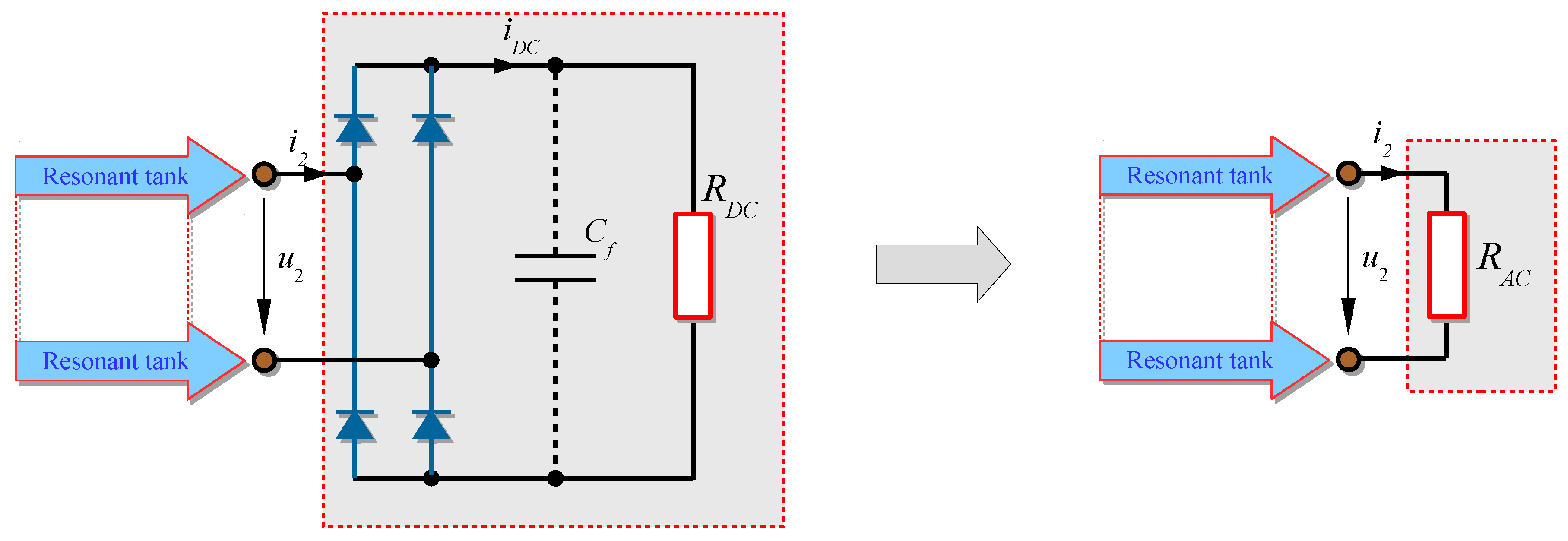
The situation may be graphically demonstrated on the WPT system transferring the power to the resistive load through the full wave bridge diode rectifier. In this case, the rectifier transforms the loading impedance from given dc value to its ac value, and therefore the load must be recalculated accordingly. It is usually done using a coefficient of impedance transformation [48] resulting in $R_{AC}=8/{\mathsf{\pi }}^2{R}_{DC}$ (see Figure 2).

The resonant tank is then described with modified set of two equations of two unknowns that are presented in Equation (17). The power on both sides may be calculated based on Equation (5).

$$\left[\begin{array}{c}{\overline{I}}_1\\ {\overline{I}}_2\end{array}\right]=\left[\begin{array}{cc}{R}_1+j\left(\omega L_1-\frac{1}{\omega C_1}\right)& -j\omega M\\ -j\omega M& R_2+j\left(\omega L_2-\frac{1}{\omega C_2}\right)+R_{AC}\end{array}\right]\backslash \left[\begin{array}{c}{\overline{U}}_1\\ 0\end{array}\right]$$

(17)

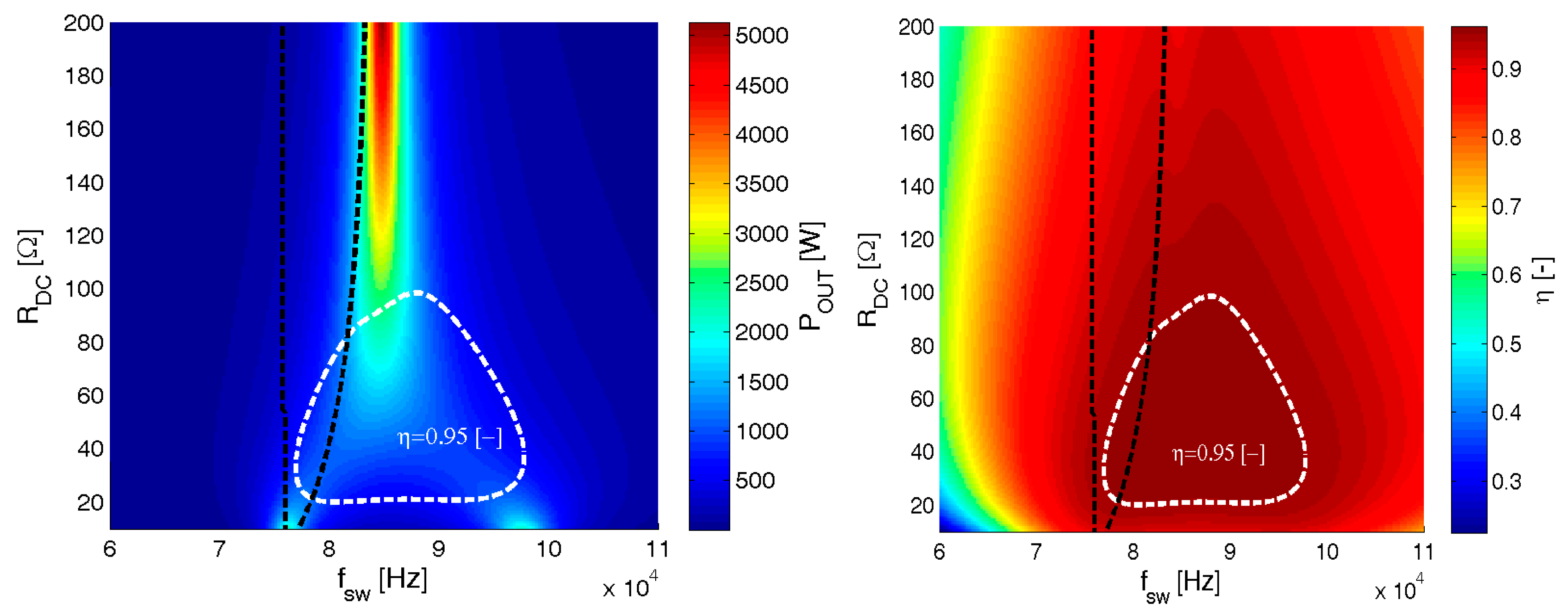
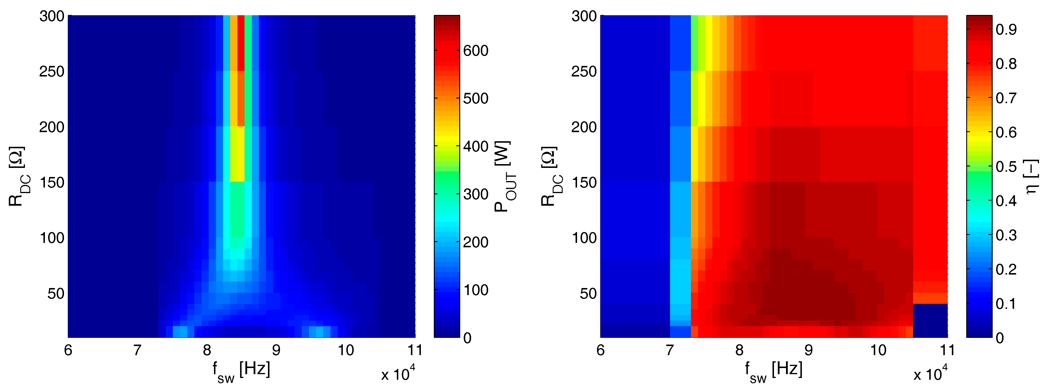
To illustrate the basic idea, a simulation of the operational output power and the efficiency needs to be performed. The results are depicted, such that the x-axis represents the operating (switching) frequency, y-axis shows the various load, and z-axis introduces observed quantity. The figures therefore represent the three dimensional plots expressed as functions of two variables (see Figure 3), e.g., P_OUT(f_sw, R_DC) and η(f_sw, R_DC). During the simulation, we assume identical coupling coils used on both the primary and the secondary side having electrical parameters, as follows. The load R_DC is considered as purely resistive, L₁ = L₂ = L = 172 μH, R₁ = R₂ = R = 0.25 Ω, and C₁ = C₂ = C = 20.5 nF. Mutual inductance M = 35 μH corresponds to the working distance 20 cm. The rectifier power loss P_RECT, which is usually referred as a conduction loss, is calculated from the diode forward characteristic as Equation (18), for details see e.g., [50,51,52]. Here, $U_F\left(\upsilon \right)$ and $I_F\left(t\right)$ are, respectively, diode forward instantaneous voltage and current, f_sw represents the switching frequency and $U_{TOD}\left(\upsilon \right)$ and $R_D\left(\upsilon \right)$ are threshold voltages and dynamic diode resistance. All of the parameters are temperature dependent ($\upsilon$). As we used SiC diodes, the switching loses can be neglected.

$$P_{RECT}=2f_{sw}{{\displaystyle \int }}_0^{\raisebox{1ex}{$1$}\!\left/ \!\raisebox{-1ex}{$fsw$}\right.}{U}_F\left(\upsilon \right)I_F\left(t\right)dt=2[U_{TOD}\left(\upsilon \right)I_{F\left(AVG\right)}+R_{DD}\left(\upsilon \right)I_{F\left(RMS\right)}^2]$$

(18)

The primary voltage-source is constructed as full-wave one-phase converter (schematically shown in Figure 6). Its power loss P_CONV is determined by using a suitable loss estimation algorithm Equation (19) widely reported in literature [38,39]. Here, $E_{on}$ and $E_{off}$ represent the switching energy of the used power electronics devices. Further, parameters U_TOS and R_DS represent the transistor saturation voltage and its dynamic resistance. Parameter I_S stands for the transistor drain-to-source current. As the converter is built from SiC MOSFET transistors, U_TOS may be considered as zero.

$$P_{CONV}=2\left[U_{TOS}\left(\upsilon \right)I_{S\left(AVG\right)}+R_{DS}\left(\upsilon \right)I_{S\left(RMS\right)}^2+\left(E_{on}+E_{off}\right)f_{sw}\right]$$

(19)

Assuming losses in the semiconductor devices, the efficiency Equation (5) changes into Equation (20).

$$\eta =\frac{P_{OUT}-P_{CONV}}{P_{IN}+P_{RECT}}$$

(20)

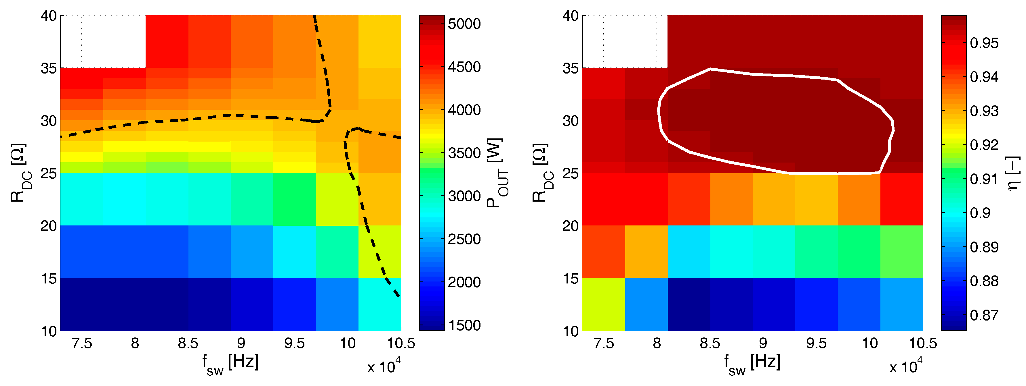
The resulting output power and efficiency are depicted in Figure 3. The white dashed line encloses the area where the efficiency is higher than 95%. The black dashed line connects all of the operational points at which the phase-shift between the primary and the secondary voltage equals to $3\mathsf{\pi }/4$.

Figure 3 shows that there is only one working point at which the efficiency culminates. This could be reach by setting the load into its optimal value Equation (7). So, the possible solution is to control the load itself, but this his approach Equation (16) works well, only in the case of fully controllable load. If the load is given by some inherent mechanism, e.g., charging cycle, then it fails. Hence, we suggest to control the working point so that it goes along the right-side of the black dashed line seen in Figure 3. At the same time, it crosses both the region of the high efficiency and the region of high transferred power.

3. Tracking Algorithm Implementation

According to the topology that is shown in Figure 4, only the phase shift $\varphi$ between primary voltage u₁ and secondary voltage u₂ is selected to represent the one degree of freedom treated as the control parameter in our approach. Independent variables are transfer distance, coupling elements misalignment, and load value. All of the other variables are considered to be constant, so we do not use any other regulation. The regulation is being implemented by controlling the switching frequency of the input full-wave one-phase inverter based on zero crossing detection of the primary u₁ and the secondary u₂ coil voltages. 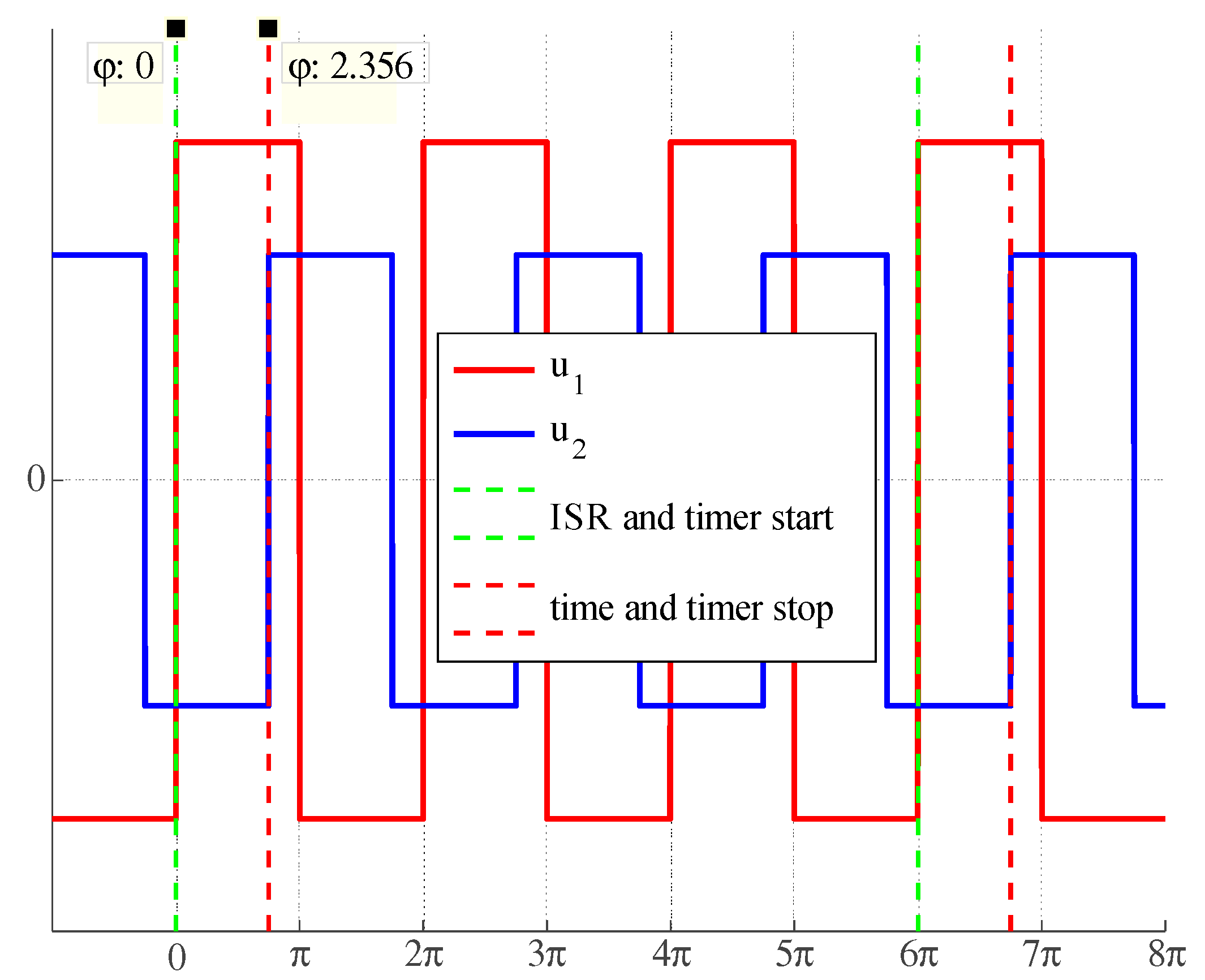In the receiver side-control loop, the phase shift angle between the voltages u₁ and u₂ can be determined using a simple method. The voltage that is induced into the air coil antenna (near electric field detector on secondary coupling element) is formed by the Schmitt trigger and is processed by the zero up crossing detection system in digital signal processor (DSP). This returns the impulse each time that the secondary coil voltage u₂ goes up through the zero. The similar impulse of the primary coil voltage u₁ goes up through the zero is generated from the interrupt service routine (ISR) of DSP PWM periphery occurring in each third time period (this impulse have clearly software character—interrupt). These two impulses are used to start and to stop the DSP timer with time based period T_timer. From the time that is measured between signals (u₁ and u₂) and primary voltage period T(u₁); we calculate the phase-shift angle ϕ as Equation (21).

The information about the time period length T is obtained from the actual setting of switching frequency in PWM peripheral in DSP. Then, we can calculate the instantaneous phase shift as

$${\varphi }_{DSP}=\frac{t\left(signal{\_}_{u_2}\uparrow -signa{l}_{u_1}\uparrow \right)}{T\left(u_1\right)}$$

(21)

The timer is reset by the rising edge of the input voltage u₁. Further, the timer counts continuously until it gets the interrupt from the rising edge of output voltage u₂. The same signal also stops the timer and records the counted value into the variable “time”. The next detected rising edge of signal u₁ begins the same timing cycle. So, hence, the timer operates in intermittent mode shown in Figure 5. As a consequence, it also reduces the computational requirements.

Based on the previous description, Equation (21) can be modified with respect to DSP implementation into Equation (22), where the quantity TBPRD is the currently set value of time base period register of PWM peripherals in DSP.

$${\varphi }_{DSP}=\frac{time}{TBPRD\frac{1}{CPUclk\times T_{timer}}}$$

(22)

The floating average Equation (23) is used to increase the algorithm stability and to reduce the frequency fluctuations of u₁.

$${\varphi }_{DSP\left(k\right)}={0.99\varphi }_{\left(k-1\right)}+0.01\left(\frac{tim{e}_{\left(k\right)}}{TBPR{D}_{\left(k\right)}\frac{1}{CPUclk\times T_{timer}}}\right)$$

(23)

With respect to Equations (21)–(23), we must set the required phase shift angle into the feedback difference block in the normalized form

$${\varphi }_{DSP}^{\ast }=\frac{\frac{3}{4}\pi }{2\pi }=0.375$$

(24)

Based on equations that are presented above, it is obvious that the switching frequency has direct influence on u₁-u₂ phase shift Equation (25). Also, the u₁-u₂ phase-shift angle equals to $\frac{\mathsf{\pi }}{2}$ when the frequency f_sw01 is applied.

$$\uparrow f_{U_1}\to \uparrow {\varphi }_{U_1-U_2}$$

(25)

According to Equation (25), the u₁−u₂ phase-shift angle can be controlled by the primary switching frequency setting. Hence, the PI phase-shift controller is implemented, as in Equation (26). Where kp is a proportional gain and ki denotes the integral gain.

$$f_{\left(k\right)}=f_{\left(k-1\right)}-kp{\left({\varphi }_{err}\right)}_{\left(k-1\right)}+\left[kp{\left({\varphi }_{err}\right)}_{\left(k\right)}+TBPRD{\left({\varphi }_{err}\right)}_{\left(k\right)}ki\right]$$

(26)

The regulation error ϕ_err is obtained from difference Equation (27) between required phase-shift angle ϕ* and the actual phase-shift angle ϕ.

$${\varphi }_{err\left(k\right)}={\varphi }_{\left(k\right)}^{\ast }-{\varphi }_{\left(k\right)}$$

(27)

The frequency range of the regulation is not wider than 10 kHz, which is in correspondence with frequency band defined by SAE TIR J2954. However, the phase-shift PI controller allows for variation of controlled frequency f, according to

$$\begin{array}{c}{f}_{max}\\ f_{min}\end{array}=f_{01}\begin{array}{c}+5e^3\\ -5e^3\end{array}\mathrm{Hz}.$$

(28)

In order to reduce the computational requirements, all of the necessary calculations together with relevant PWM settings are made during interrupt services routine (ISR) of each third PWM period (see Figure 5).

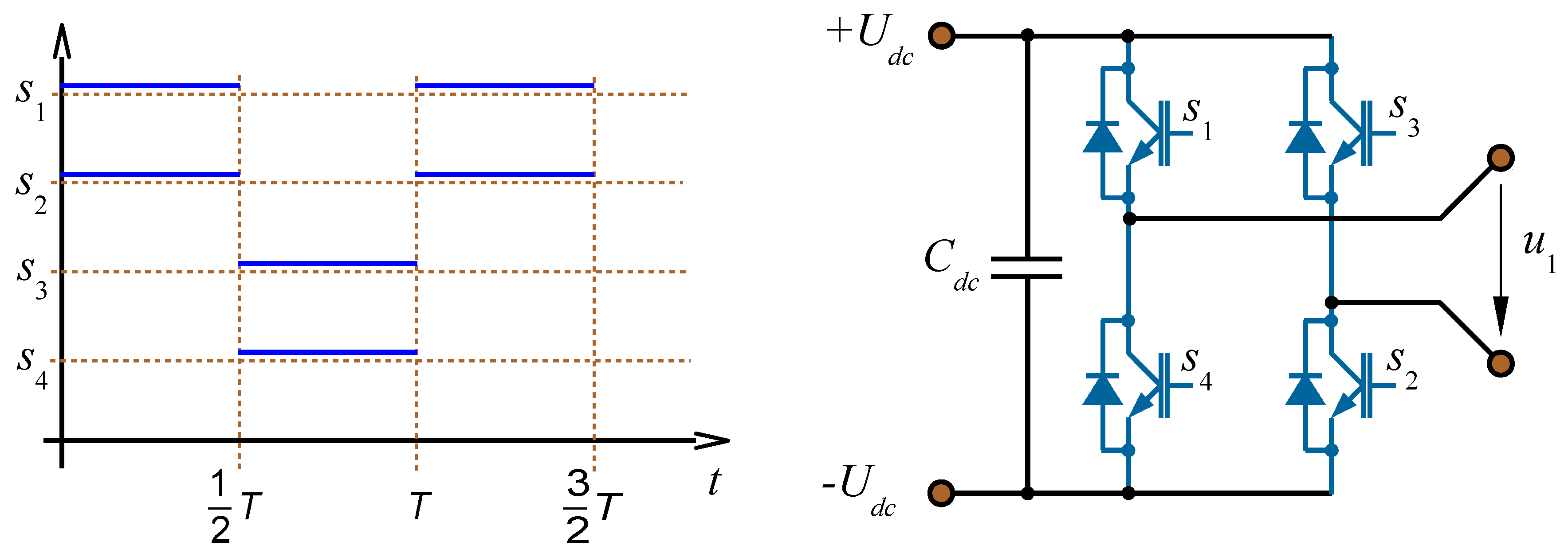
The PWM peripheral generates switching signals to get bipolar rectangular-shape voltage u₁ with 50% duty cycle. The situation is clear from the switching diagram and the voltage-source inverter configuration shown in Figure 6.

4. Experimental Prototype Description

The WPT experimental prototype consists of a couple of planar square shaped coils with external dimensions 0.5 m × 0.5 m. The square-shape for the coils is chosen in order to reach maximum possible self-inductance. The windings have 22 coil turns wound from RF cable having 2200 insulated strands of total cross-section area that is close to 20 mm². The diameter of each strand is smaller than the skin depth; hence, the skin effect has no influence on the resulting series coil resistance. The coil windings are evenly distributed in one layer with a constant 4mm spacing to prevent high parasitic capacitance. In order to get large operational quality of the resonant tank, we used high-quality RF high-power ceramic capacitors to compensate the leakage inductance. All of the parameters are identical to those that are used in the previous theoretical discussion, i.e., L₁ = L₂ = L = 172 μH, R₁ = R₂ = R = 0.25 Ω, and C₁ = C₂ = C = 20.5 nF.

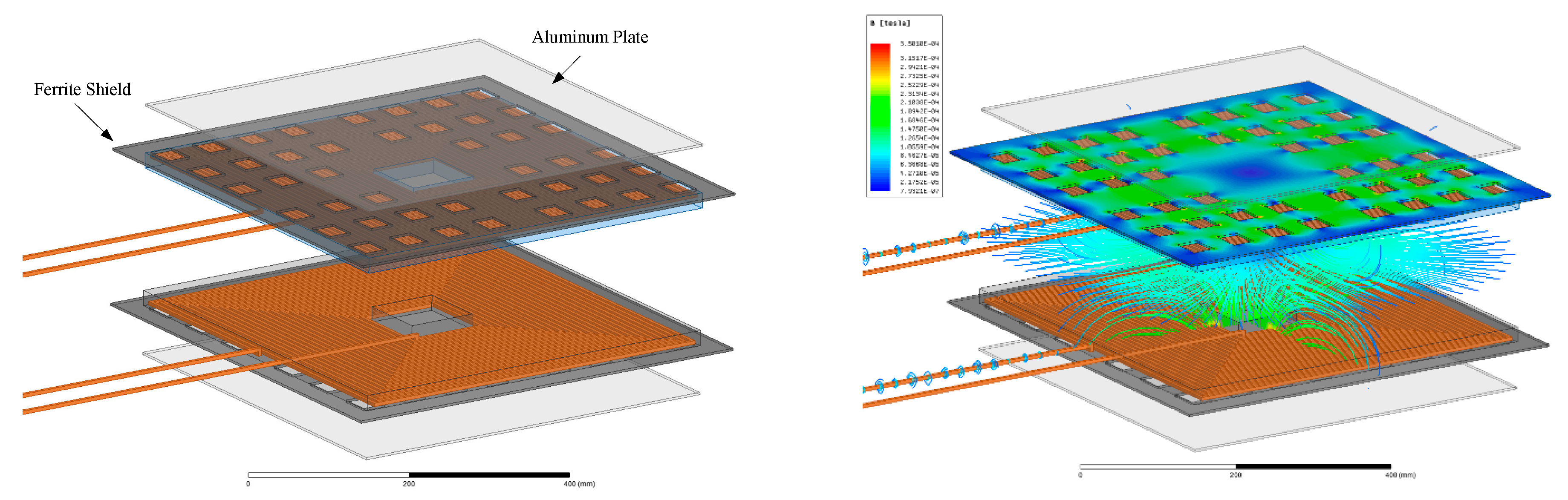
Additional electro-magnetic (EM) shielding uses the benefits of both the electric and magnetic shielding mechanisms into one functional block. The magnetic shield is constructed as a matrix-arrangement of high magnetic permeability ferrite cores (material N87) lying on the back coil sides. It provides a preferential path for the magnetic flux lines, and therefore, the magnetic field is guided mainly into the air gap space and the vehicle cabin remains protected from any leaked EM field. A conductive aluminum panel located in a certain distance over the ferrite shielding is used as a second stage of shielding. Remaining EM field that leaks through the magnetic shield will induce eddy currents into the aluminum plate, which create a magnetic field that is opposite to the incident one. As a consequence, the leaked magnetic field will not get out of the active zone of the coupling coils. The situation is demonstrated in Figure 7.

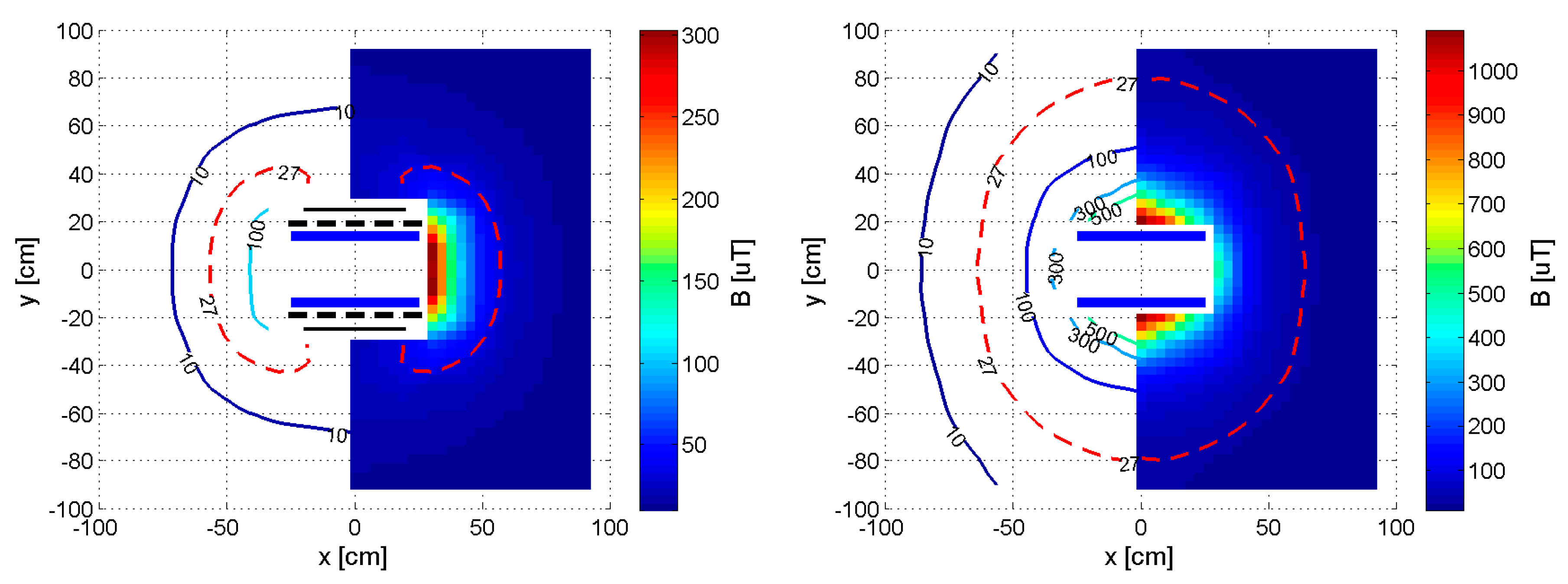
Magnetic field measured with the exposure-level-tester ELT 400 (Narda Safety Test Solutions) is presented in Figure 8. The magnetic field has been measured around the coupling coils when delivering 4 kW of power to the load. While the left-side figure shows the shielded system, the right-side figure shows the unshielded system. The limiting field level (27 μT), defined by International Commission on Non-Ionizing Radiation Protection stablished in guidelines ICNIRP 2010 [9] for public exposure, is outlined with dashed red line. As it is obvious, the proposed shielding significantly suppresses the magnetic field in the vehicle cabin direction, and can therefore be evaluated as effective.

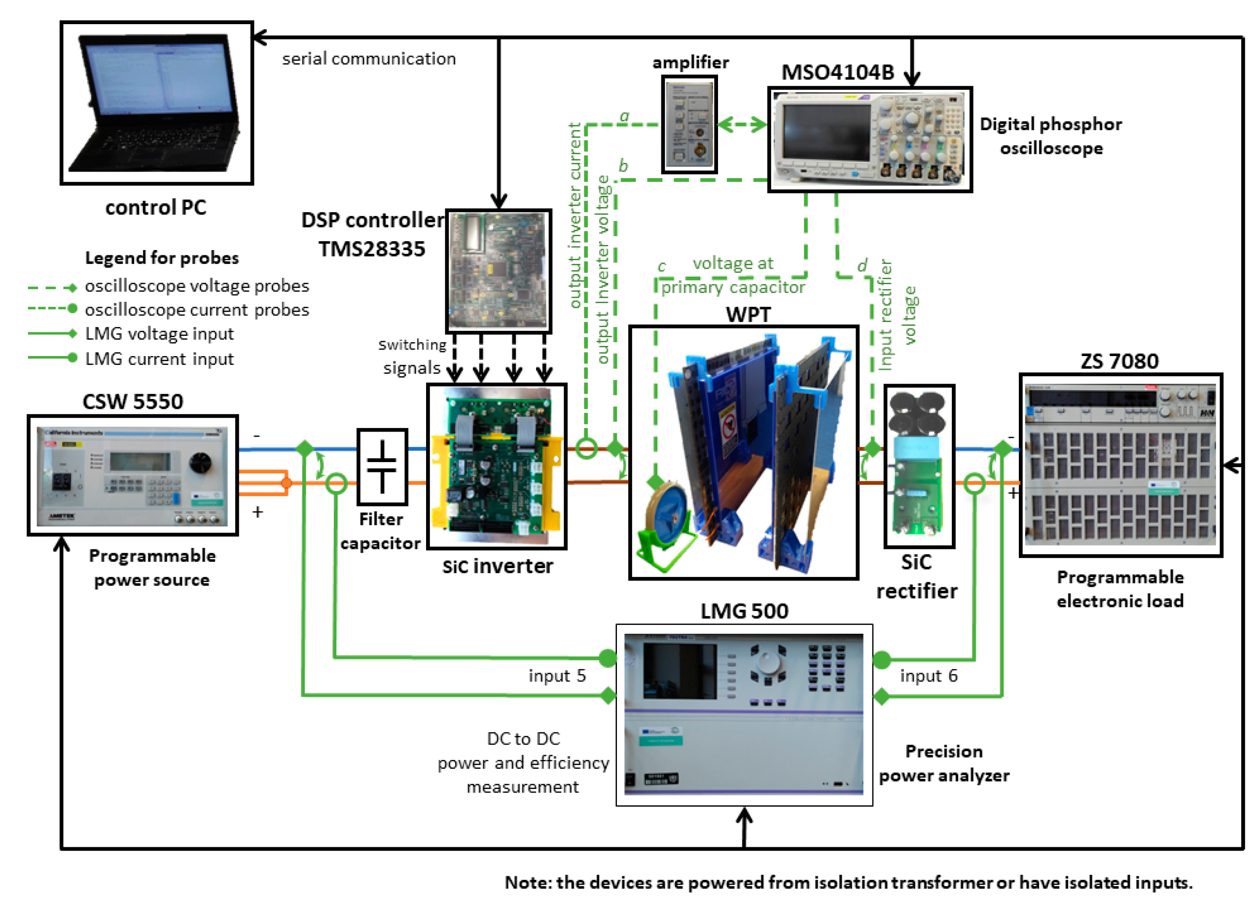
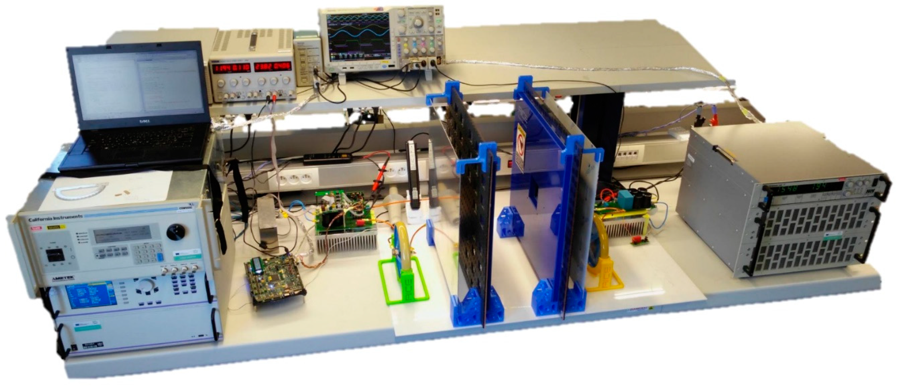
An experimental WPT setup consists of a programmable dc source CSW 550 (AMETEK), electronic load GmbH ZS 7080 (Höcherl & Hackl GmbH), precise power analyzer LMG 500 (ZES ZIMMER Precision Power Measurement), oscilloscope TEKTRONIX MSO4104B, designed input full-SiC voltage-source inverter, WPT coils with series-series compensated resonant tank and the output rectifier. It is installed according to the functional diagram that is introduced in Figure 9. The input inverter is designed as a single-phase inverter (H-bridge), and according to originally required high switching frequency it is based on the SiC devices 1200 V JFET modules FF45R12J1W1_B11 (Infineon) with a nominal current of 45 A. Short switching times of these SiC modules (tens of ns) significantly minimize the impact of the dead-times. The output rectifier is also based on SiC technology and uses 1200 V diode modules APTDC20H1201G (Microsemi) with rated current of 20 A.

Three quantities on the primary side are measured with the oscilloscope, but this measurement is rather indicative and it is not used for efficiency calculation. Probe “b” THDP 0200 (Tektronix) measures the inverter output voltage (primary coil voltage u₁), probe “a” (TCP 404 XL current probe and TCPA 400 amplifier) measures the primary coil current, probe “c” (P6015A) senses voltage drop on the input coil compensating capacitor and probe “d” (THDP 0200) measures the rectifier input voltage (secondary coil voltage u₂). The overall system efficiency (DC-DC) is calculated by precise power analyses LMG 500 (ZES ZIMMER Precision Power Measurement) while using DC voltages and currents on the source and load sides. Hence, the efficiency considers the power loss that is generated in the input inverter, the resonant tank, and the output rectifier. The laboratory prototype of the WPT system is shown in Figure 10.

5. Experimental Measurement

Validation of the proposed tracking algorithm has been done on experimental prototype of the WPT system described in the previous section (see Figure 9 and Figure 10). A special attention has been paid to the measurement accuracy, all of the measuring devices have been calibrated by external certified authority. For example, decelerated accuracy of precision power analyzer ZIMMER LMG 500 is 0.018% of the used scale for currents an 0.034% of the used scale for voltages. High accuracy is required mainly when measuring the input and output DC voltages and currents that are used for the system efficiency calculation. To avoid any human factors from the analyses, the measurement procedure is fully automatic, driven by control PC. Operational distance or possible coils misalignment (changes of mutual inductance) must be arranged manually. The input and the output dc powers are measured by the LMG 500. The processed data are then stored into the PC memory to be ready for the future processing. The PC also secures serial communication between all measuring devices and based on the measuring script performs any changes in the measurement settings while also using serial communication.

The proposed tracking algorithm runs on DSP TMS 28335 (v7). The proper frequency settings are done by the control computer, according to the actual phase-shift angle between the primary and the secondary voltages. The signal corresponding to the secondary voltage is given, as follows. One logical input is general purpose input output (GPIO) with zero crossing detection. As mentioned in paragraph 3 and Figure 4, the signal for this input is sensed somewhere close to the secondary coupling coil from its EM field while using primitive antenna.

Besides that, the control computer collects all other important quantities, such as DC input and output voltages, currents, and powers. The only predefined parameter is the load value (electronic load resistance) that is set for each measurement point.

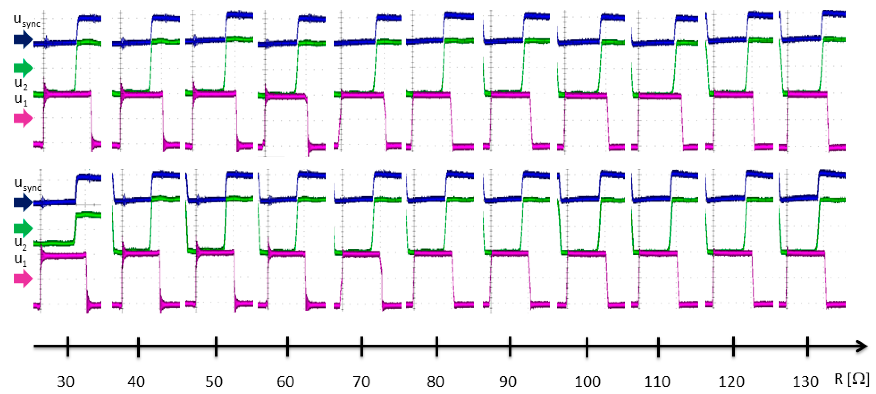
Figure 11 compares the phase shift values observed in the system with (bottom) and without (upper) application of the proposed tracking algorithm ($\varphi =\frac{3}{4}\mathsf{\pi }$). The curve u_sysnc represents the voltage outgoing from block “u₂ former” shown in Figure 4. It is obvious that the load variation leads to the consequent switching frequency change.

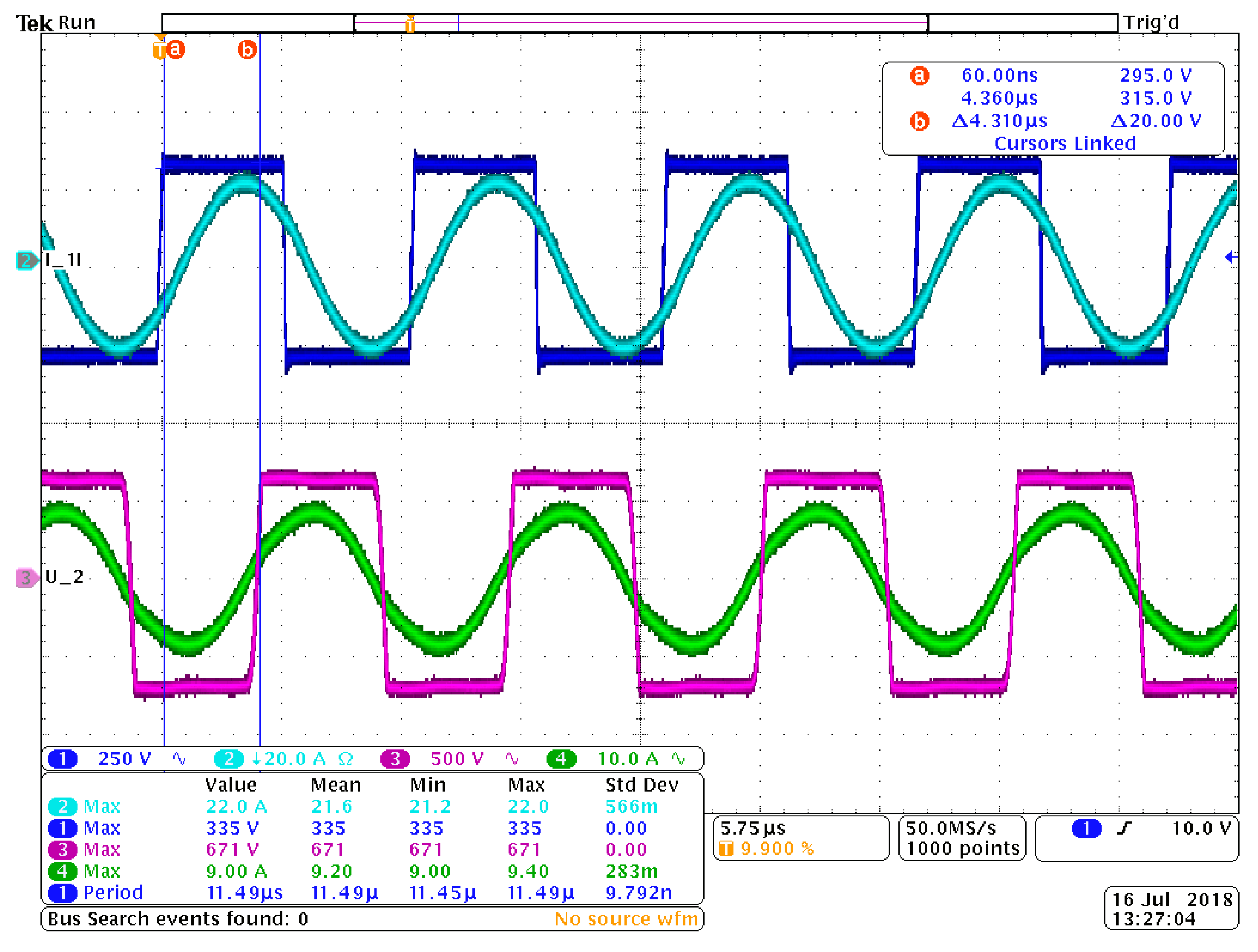
Instantaneous quantities (voltages and currents) that were measured on both AC sides are seen in Figure 12. It shows the primary voltage (dark blue), the primary current (light blue), and the secondary voltage (magenta) and the secondary current (green) with regulation ϕ = ¾ π (marked with cursors). Actual operating conditions are as follows: R_AC = 120 Ω, transfer distance 200 mm, power delivered to the load is 3950 W.

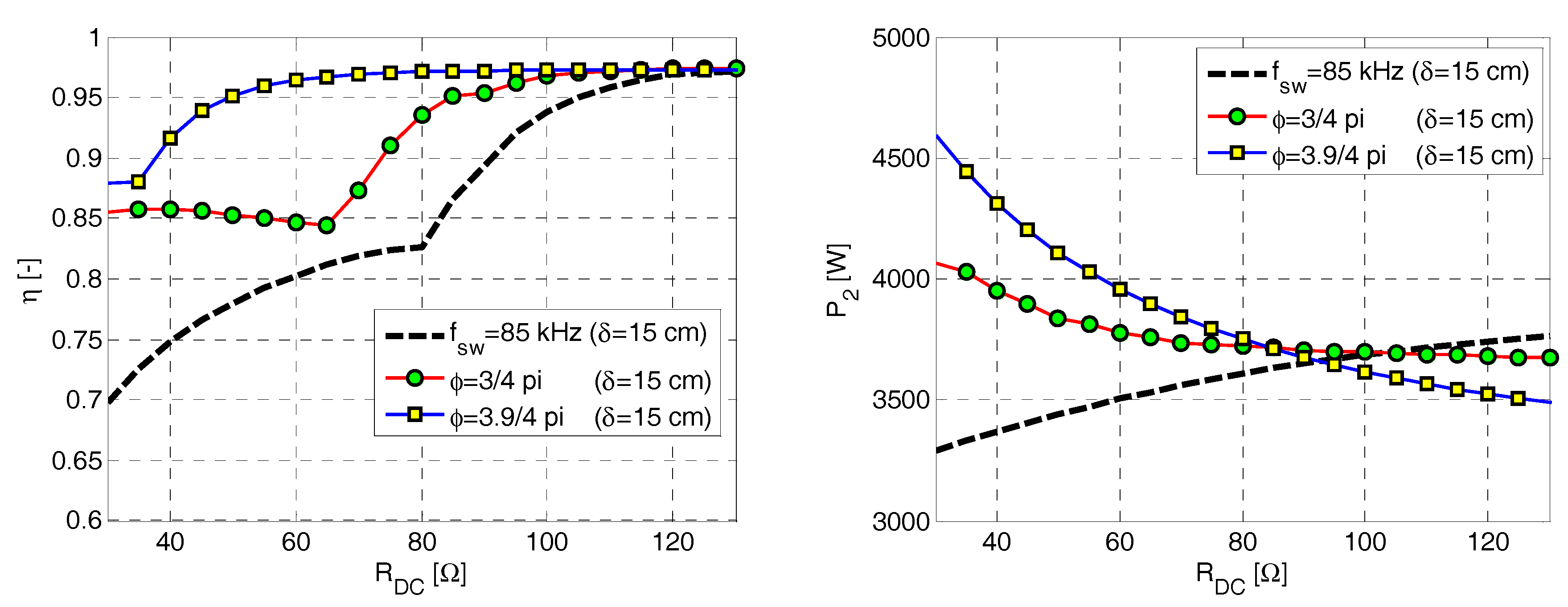
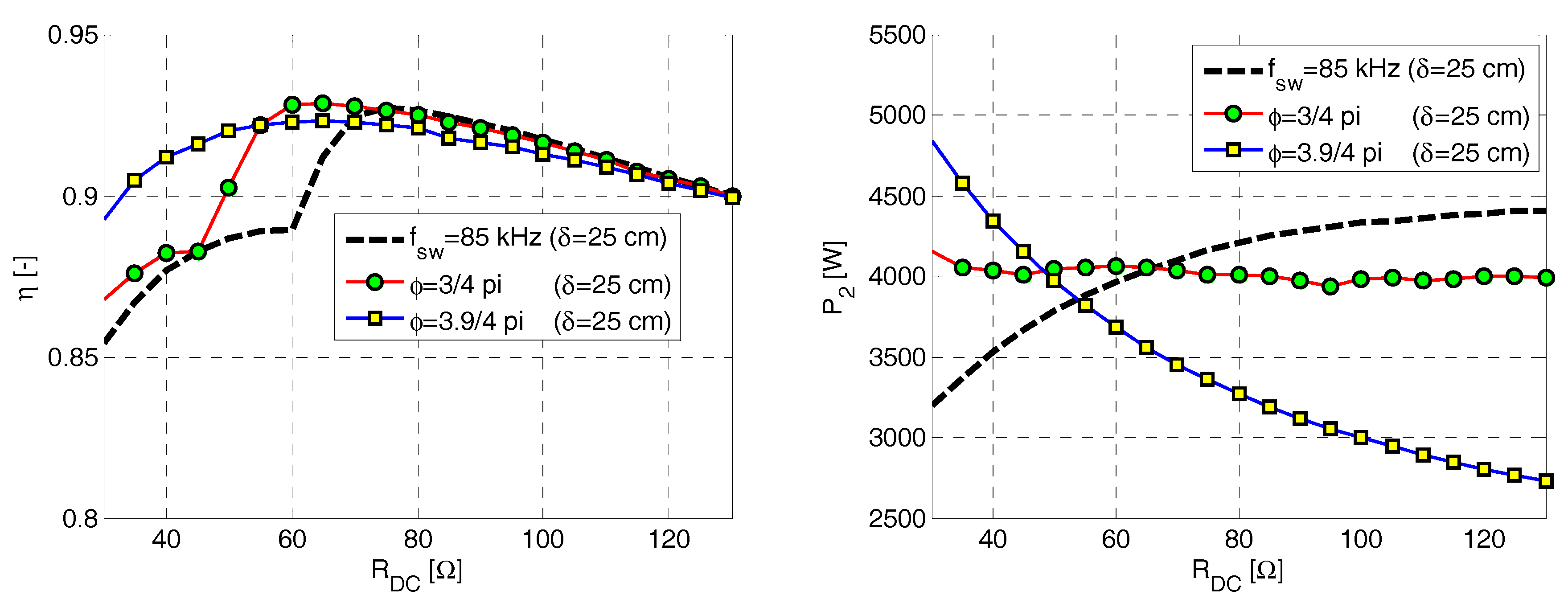
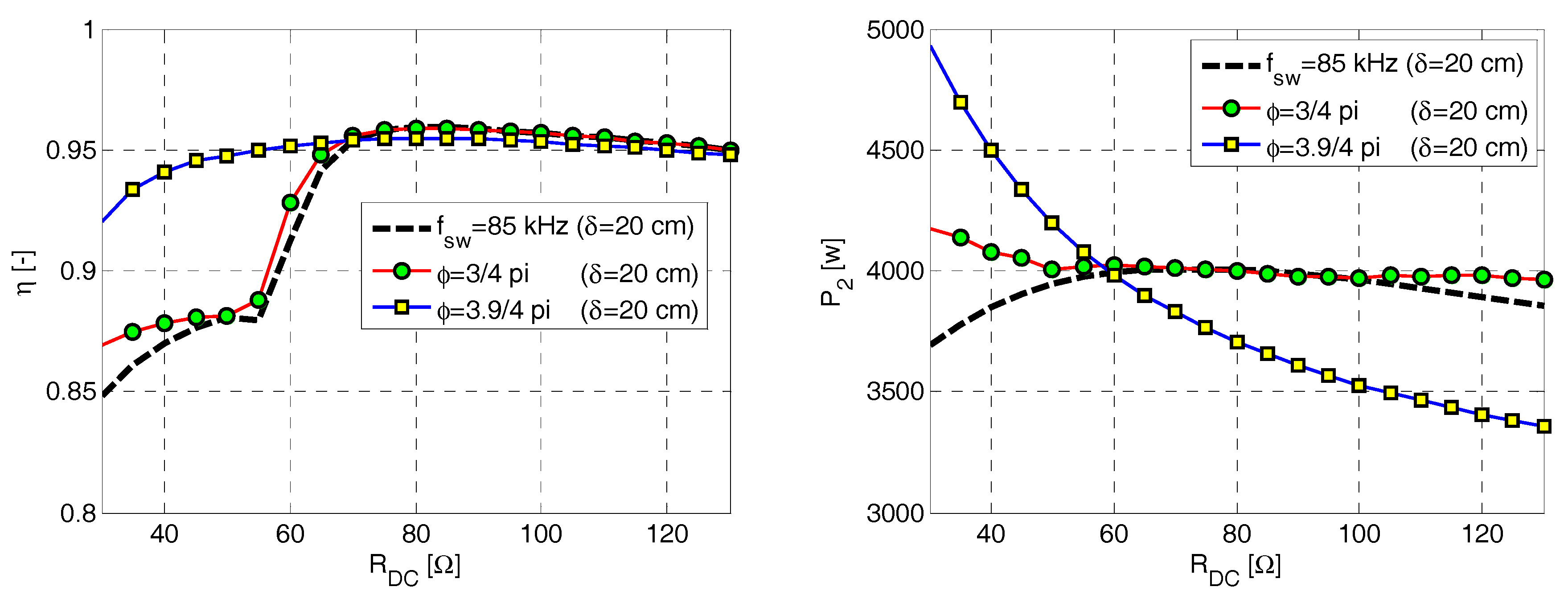
The situation may be easier understood from Figure 13, Figure 14 and Figure 15. They compare the measured values for three chosen working distances (15, 20, and 25 cm). The left side of figures shows the overall system efficiency in per-units (left side of Equation (29)) and the right side depicts the power delivered to the load. The red curves with circle marks plot the values obtained when the proposed control method is applied, the blue curves with the yellow-square marks represent the same control but with modified setting of $\varphi =\frac{3.9}{4}\mathsf{\pi }$ Finally, data corresponding to the fixed switching frequency operation (85 kHz) are illustrated with the black dashed lines.

$$\eta [-]=\frac{P_2}{P_1}\le 1;\cdots \eta [\%]=100\frac{P_2}{P_1}\le 100$$

(29)

According to the paragraph 2 and especially with consideration (6) ÷ (8), unregulated system resonates on main resonant frequency f_sw01 when optimal load is applied. In that case, the system reaches high operational efficiency. This assumption is confirmed by Figure 12, Figure 13 and Figure 14. Delivered power to the load can be also called optimal in this case.

Further, in case of load values that are lower than the optimal load, the system resonates on the side-band resonant frequencies f_sw02 and f_sw03, so hence, in the case of unregulated system, the load power and efficiency must rapidly decrease.

On the other hand, according to the paragraph 2 and (24) ÷ (25), the regulated frequency is always higher than the main resonant frequency.

The aim of proposed regulation method ($\varphi =\frac{3}{4}\mathsf{\pi }$) is to hold the optimal power and maximal possible efficiency across the wide range of the load values and transferring distances. With using the proposed method, the transmitted power is practically constant and the efficiency is always the same or higher than in case of unregulated system.

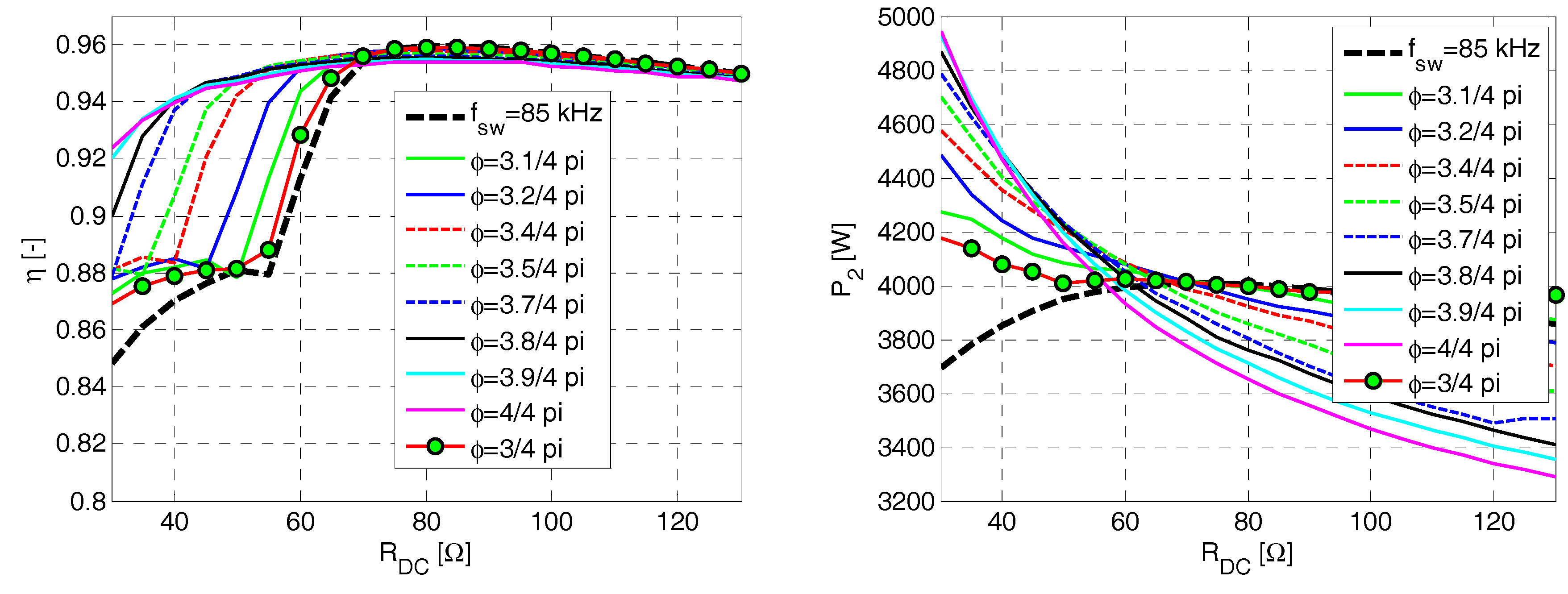
Side-effect benefit of the proposed tracking algorithm comes with higher ϕ*. In this case, the system works closer to the right-band resonant frequency where it reaches high power transferred only for lower loads (according to the Figure 2 and Figure 16). This brings behavior that is nearly opposite to the curves that were recorded for uncontrolled system and should be taken as an advantage when optimizing the WPT for low values of the load.

As reported in left-side figures and text, the proposed algorithm positively effects the efficiency, which is significantly improved, especially at the operation with the low values of the load. More detailed results are shown in Figure 16.

Full operational maps measured at reduced (lower input voltage) load power are shown in Figure 17. The results are measured with equipment seen in Figure 10 and interpreted in the same way as presented in Figure 3. The presented operational maps are collected from sequential measurement of non-regulated system for various switching frequency and load and correspond to the shielded system working with 20 cm air gap. From obtained results, we can find good agreement between experimental and simulation data. The simulation that is seen in Figure 3 is based on (17) ÷ (20) and it is implemented into a Matlab (R2017) code.

The system ability to transmit high power to the load can only be demonstrated in a limited operational region (close to resonance). The reason is a great power variation for the entire considered load range and a high consequent probability of destroying the input inverter in the marginal areas of the map. Therefore, the detail of the area with the maximum efficiency is presented in Figure 18. The black dashed curves on the left side represent the lines where the power is equal to 4 kW and the white line on the right side encloses the area with the efficiency being over 95%.

6. Conclusions

The optimal operating point tracking algorithm for wireless charging system is proposed in this paper to provide excellent characteristics of WPT system.

The advantage of the algorithm is the ability to meet simultaneously high efficiency and high transmitted power under varied load and detuning conditions. Given mathematical description has shown good coincidence with the experimental measurement.

It was found that the uncontrolled system resonates at three different frequencies, which are moreover dependent on load and the working distance. As a consequence, the system is unable to operate simultaneously with the maximum efficiency and maximum power. The power changes strongly together with the load variation, but for practical usage, it is better to have a stable power source. In order to improve its operational ability, the phase shift between the primary and secondary voltages has been controlled so that it is equal to $3\pi /4$. The phase shift control is achieved by adjustment of the switching frequency of the input single-phase inverter. The switching frequency control utilizes zero crossing detection of the primary u₁ and the secondary u₂ coil voltages (see Figure 4).

As confirmed by the experiment, the proposed algorithm fully compensates any change of power across the wide range of load by careful switching frequency adaptation. The control with $\varphi =\frac{3}{4}\mathsf{\pi }$ provides us with constant output power, almost independent of the load and the working distance. The control with $\varphi =\frac{3.9}{4}\mathsf{\pi }$ brings behavior that is nearly opposite to the curves that were recorded for uncontrolled system. This could be taken as an advantage when optimizing the WPT for low values of the load. The proposed algorithm positively effects also the efficiency, which is significantly improved, especially at the operation with the low values of load (very important for application in battery charging systems).

The electromagnetic compatibility issue has been discussed as well. The WPT system includes additional EM shielding with the benefits of both the electric and magnetic shielding mechanisms integrated into one functional block (see Figure 7). Flux density measurements of WPT system with/without EM shielding are presented in Figure 8. The magnetic field is measured around the coupling coils when delivering 4 kW of power to the load. The limiting field level (27 μT), as defined by ICNIRP 2010 for public exposure, is outlined with a dashed red line. As it is obvious, the proposed shielding significantly suppresses the magnetic field in the vehicle cabin direction and can therefore be evaluated as effective.