The Efficiency of Long-Term Forecasting Model on Final Energy Consumption in Thailand’s Petroleum Industries Sector: Enriching the LT-ARIMAXS Model under a Sustainability Policy

Abstract

Presently, Thailand runs various sustainable development-based policies to boost the growth in economy, society, and environment. In this study, the economic and social growth was found to continuously increase and negatively deteriorate the environment at the same time due to a more massive final energy consumption in the petroleum industries sector than any other sectors. Therefore, it is necessary to establish national planning and it requires an effective forecasting model to support Thailand’s policy-making. This study aimed to construct a forecasting model for a final energy consumption prediction in Thailand’s petroleum industry sector for a longer-term (2018–2037) at a maximum efficiency from a certain class of methods. The Long Term-Autoregressive Integrated Moving Average with Exogeneous variables and Error Correction Mechanism model (LT-ARIMAXS model) (p, d, q, Xi, ECT_(t−1)) was adapted from the autoregressive and moving average model incorporating influential variables together in both long-term relationships to produce the best model for prediction performance. All relevant variables in the model are stationary at Level I(0) or Level I(1). In terms of the extraneous variables, they consist of per capita GDP, population growth, oil price, energy intensity, urbanization rate, industrial structure, and net exports. The study found that the variables used are the causal factors and stationary at the first difference as well as co-integrated. With such features, it reflects that the variables are influential over the final energy consumption. The LT-ARIMAXS model (2,1,2) determined a proper period (t − i) through a white noise process with the Q test statistical method. It shows that the LT-ARIMAXS model (2,1,2) does not generate the issues of heteroskedasticity, multicollinearity, and autocorrelation. The performance of LT-ARIMAXS model (2,1,2) was tested based on the mean absolute percentage error (MAPE) and the root mean square error (RMSE). The LT-ARIMAXS model (2,1,2) can predict the final energy consumption based on the Sustainable Development Plan for the 20 years from 2018 to 2037. The results showed that the final energy consumption continues to increase steadily by 121,461 ktoe in 2037. Furthermore, the findings present that the growth rate (2037/2017) increases by 109.8%, which is not in line with Thailand’s reduction policy. In this study, the MAPE was valued at 0.97% and RMSE was valued at 2.12% when compared to the other old models. Therefore, the LT-ARIMAXS model (2,1,2) can be useful and appropriate for policy-making to achieve sustainability.

1. Introduction

Thailand has continuously put efforts into accelerating the economic development of the country by focusing on widening urbanization. In parallel, the government is trying its best to encourage both domestic and international private investment. This is to ensure that the industrial structure is broadened. At the same time, Thailand is also focusing on export activities where Thailand is to be a production base, so that Thailand’s market share will continue to expand. Additionally, there are also policies designed to increase spending, attract more foreign tourists and increase the minimum wage rate, resulting in the increments of both local and foreign labors. Therefore, these policies have supported the Thai economy to grow with a 4.3% growth rate in 2016/2017 [1], and a 2.5% population growth rate (2016/2017) [2]. However, the economic and population growth in Thailand has continuously caused the environment to deteriorate. In 2017, CO₂ emissions from energy consumption increased by 1.3% when compared to 2016 [3]. These CO₂ emissions are highly contributed by the petroleum industries sector, accounting for 50.1% of the final energy consumption (2017). In fact, the final energy consumption has resulted in continuous economic growth, and that growth has also been affected by inflation due to the constant increase of world oil prices [1,3]. In addition, 89% of carbon dioxide is released by the energy sector with a growth rate of 10.3% (2016/2017). The petroleum industries sector produces more CO₂ due to its maximal power consumption. This reflects the fact that the above sector releases the most greenhouse gas. Emissions are expressed in the form of CO₂ (with the highest emissions) as well as other gases including methane (CH₄), nitrous oxide (N₂O), hydrofluorocarbons (HFC), perfluorocarbons (PFC), sulfur hexafluoride (SF₆), and nitrogen trifluoride (NF₃) [4,5].

The sustainable development policy is the future policy that Thailand aims to achieve. The focus of the policy covers three main areas: economic growth, social growth, and environmental growth. The policy is achieved when those three areas are simultaneously developed. For Thailand, both short-term (five years) and long-term (20 years) plans have been set [1]. Nonetheless, the implementation of Thailand’s sustainable development policy results in growth in both the economy and population. This also affects the increment of energy consumption. Thus, Thailand has set a long-term reduction goal of 20 years (2018–2037) in the final energy consumption based on the petroleum industries sector not exceeding 90,000 ktoe [3]. This is because the petroleum industries sector accounts for highest energy consumption (50.1%) and produces most of the greenhouse gases [5]. Therefore, the most important tool in effective policy planning for sustainability is to forecast the future possibility [3,5].

However, the best forecasting model on energy consumption must also be able to support sustainable development policy planning. From the various relevant studies that have been reviewed, there are different models and forecasting techniques optimized for different forecasting timelines, be it short-term or long-term. Therefore, it is necessary to examine what has been done in this area to increase the quality of the proposed model. In fact, there have been few stream studies exploring total energy consumption. For instance, Zhao, Zhao, and Guo [6] started to estimate the electricity consumption of Inner Mongolia by deploying gray model (GM(1,1) model) optimized by moth-flame optimization (MFO) with a rolling mechanism from 2010 to 2014. Their study indicated which model could improve the forecasting performance of annual electricity consumption significantly. Li and Li [7] also initiated a comparative study by using the autoregressive integrated moving average model (ARIMA model), GM(1,1) model, and ARIMA–GM model to forecast energy consumption in Shandong, China from 2016 to 2020. Their prediction results showed that the energy demand of Shandong Province between those years would increase at an average annual rate of 3.9%. Similarly, Xiong, Dang, Yao and Wang [8] proposed a novel GM(1,1) model based on optimizing the initial condition in accordance with the new information priority principle to predict China’s energy consumption and production from 2013 to 2017. The study produced findings indicating that China’s energy consumption and production will keep increasing, as will the gap between them. Furthermore, Panklib, Prakasvudhisarn, and Khummongkol [9] attempted to forecast electricity consumption in Thailand by using an artificial neural network and multiple linear regression model (MLR model) for the years 2010, 2015, and 2020. Their estimation revealed that the electricity consumption of Thailand in 2010, 2015, and 2020, retrieved from the regression, would reach 160,136, 188,552, and 216,986 GWh, respectively, whereas 155,917, 174,394, and 188,137 GWh were the results obtained from the artificial neural network model (ANN model). Additionally, an ANN integrated with genetic algorithm was also presented by Azadeh, Ghaderi, Tarverdian, and Saberi [10] to estimate the electricity consumption in the Iranian agriculture sector in 2008. They observed that the integrated genetic algorithm (GA) and ANN model dominated the time series approach, yielding less mean absolute percentage error.

By incorporating values of socio-economic indicators and climatic conditions, Günay [11] modeled artificial neural networks with the use of predicted values of socio-economic indicators and climatic conditions to predict the annual gross electricity demand of Turkey in 2028, which produced a result where the demand would double, accounting for 460 TW in 2028, when compared to the years 2007 to 2013. Dai, Niu and Li [12] explored energy consumption forecasting in China from 2018 until 2022 by adopting a model of ensemble empirical mode decomposition and least squares support vector machine with the technology of the improved shuffled frog leaping algorithm. Their results showed China’s energy consumption to have a significant growth trend. Based on Wang and Li [13], they tried to find whether China’s coal consumption during 2016 to 2020 would be higher or lower than the level of 2014. Here, they optimized a time series model with a comprehensive analysis of data reliability. According to the analysis, it indicated that the annual Chinese coal consumption during 2016–2020 would be lower than the level of 2014 provided the annual average GDP growth rate was less than 8.2% per year. Suganthi and Samuel [14] developed econometric models to study the influence of the socioeconomic variables on energy consumption in India from 2030 to 2031 and found that the electricity demand depended on the Gross National Product (GNP) and electricity price, and the total energy requirement was found to be 22.944 × 10¹⁵ kJ.

In addition, Xu et al. [15] analyzed the change of energy consumption and CO₂ emissions in China’s cement industry and its driving factors over the period between 1990 to 2009 by applying a log-mean Divisia index (LMDI) method. With such analysis, the study reveals that, by applying the best available technology, an additional energy saving potential of 26% and a CO₂ mitigation potential of 33% can be gained when compared with 2009. Kishita, Yamaguchi, and Umeda [16] tried to analyze electricity consumption in the telecommunications industry in 2030 by deploying an electricity demand model for the telecommunications industry (EDMoTI). The prediction results pointed out that electricity consumption in 2030 would be 0.7–1.6 times larger than the level of 2012 (10.7 TWh per year). For a shorter time of prediction, Zhao, Wang and Lu [17] conducted a study to forecast the monthly electricity consumption in China by proposing a time-varying-weight combining method: the High-order Markov chain based time-varying weighted average (HM–TWA) method. Their forecasting performance evaluation showed that the HM–TWA produced a better outcome for the component models and traditional combining methods.

Nonetheless, several studies have examined the total energy demands and its consumption for a longer term of forecasting. For instance, Hamzacebi and Es [18] implemented optimized grey modeling to forecast the total electric energy demand of Turkey from 2013 to 2025. Their prediction reflected that the direct forecasting approach resulted in better predictions than the iterative forecasting approach in estimating the electricity consumption in Turkey. An Improved Gray Forecast Model was also drawn by Mu et al. [19] to predict CO₂ emissions, energy consumption, and economic growth in China from 2011 and 2020 by using an improved grey model. Based on their prediction results, China’s compound annual emissions, energy consumption, and real GDP growth for the predicted years was found to be 4.47–0.06% and 6.67%, respectively. Furthermore, Zeng, Zhou, and Zhang [20] proposed a Homologous Grey Prediction Model to predict the energy consumption of China’s manufacturing from 2018 to 2024 where their study revealed that the total energy consumption in China’s manufacturing was slowing down, however, the amount was still too large. Additionally, Jiang, Yang and Li [21] adapted a metabolic grey model (MGM), ARIMA model, MGM–ARIMA model, and back propagation neural network (BP) to forecast energy demand from 2017 to 2030. From their estimation, it showed that India’s energy consumption would increase by 4.75% a year in the next 14 years at a 5% growth rate. By using the same, but improved, forecasting model, Ediger and Akar [22] analyzed the primary energy demand by fuel in Turkey from 2005 to 2020 using the ARIMA model and seasonal ARIMA (SARIMA) methods to estimate the above demand, and showed that the average annual growth rates of individual energy sources and total primary energy would decrease in all cases, except wood, and the animal–plant went negative.

Furthermore, Ekonomou [23] developed an artificial neural network to estimate the Greek long-term energy consumption from 2005 to 2008, 2010, 2012, and 2015. Overall, the study has constituted an accurate tool for the forecasting problem in Greek long-term energy consumption. In addition, Ardakani and Ardehali [24] utilized an IPSO (improved particle swarm optimization)–ANN model to forecast EEC (electrical energy consumption) for Iran and the U.S. from 2010 to 2030, which resulted in the mean absolute percentage error of 1.94% and 1.51% for Iran and the U.S., respectively. In the context of Thailand, a study of characteristics and factors towards energy consumption was conducted by Supasa et al. [25], who explored five household group energy consumption characteristics and seven driving forces of growth in residential energy consumption from 2000 to 2010 by applying the energy input–output method. Their calculations indicated that about 70% of total residential energy consumption was indirect energy consumption from consuming products and services. Seung et al. [26] predicted the future electricity demand for cooling in the building sectors in Singapore from 2014 to 2030 by applying a MLR model. Their study revealed that the electricity demands accounted for 31 ± 2% of the total electricity consumption in Singapore. Additionally, Wang et al. [27] attempted to estimate the total industrial energy consumption and energy-related carbon emissions in Tianjin from 2003 to 2012 by using an energy decomposition analysis. From their evaluation, energy efficiency could be enhanced by energy-saving efforts and the optimization of the industrial structure.

In fact, Zou, Liu, and Tang [28] analyzed the factors that contributed towards the changes in energy consumption in Tangshan city from 2007 to 2012 by applying the logarithmic mean Divisia index. Their findings showed that the technical effect played a vital role in reducing energy consumption in most sectors. Another investigation of the impacts of urban land use on energy consumption in China from 2000 to 2010 was undertaken by Zhao, Thinh, and Li [29]. They used a panel data analysis with nighttime light (NTL) data estimation. Their study on sigh has shown that an increase in the irregularity of urban land forms and the expansion of urban land will accelerate energy consumption, which indicates the relationship between urban growth and energy consumption. Similarly, Tian, Xiong, and Ma [30] evaluated the potential impacts of China’s industrial structure on energy consumption by deploying a fuzzy multi-objective optimization model based on the input–output model from 2015 to 2020. From their analysis, they concluded that the industrial structure adjustment had great potential in energy conservation, and such an adjustment could save energy by 19% (1129.17 Mtce) at the average annual growth rate of 7% GDP. Ayvaz and Kusakci [31] employed a nonhomogeneous discrete grey model (NDGM) to forecast electricity consumption from 2014 to 2030. In their findings, they proved that the grey model proposed produced a better forecasting performance.

Previous studies have used varied methodologies and analyses, while the forecasting timeline includes short-term (1–5 years), mid-term (6–10 years), and long-term (11–20 years). From this point of view, only few studies have been conducted for long-term forecasting, accounting for about 28% out of the reviewed research. Moreover, the long-term forecasting studies are very limited, and that limitation may result in lower quality when compared to short-term and mid-term studies. From the study of related research on prediction models, we have found some shortcomings in long-term forecasting including a lack of true variable selection for a causality based on context and study interest, a lack of co-integration test and the error correction mechanism test, and a lack of a spurious test. In addition, those models did not identify the problems of heteroskedasticity, multicollinearity, and autocorrelation. In the context of Thailand, in the past, most energy consumption forecasting models used were of those models adapted from traditional approaches such as the Ordinary Least Square (OLS) model, the Autoregressive Moving Average (ARMA) model, the ARIMA model, and the ANN model. In fact, the above models were for forecasting with potentially high errors. They did not consider the causal variables in the real context of Thailand. Therefore, the influence of the factors towards dependent variables were unknown. When the output was used in national policy-making, this would negatively affect the country at large. However, the models are for short-term forecasting [5]. These models cannot be used for national long-term policy-making. As a result, the country has failed to head in the right direction for achieving the reduction goal and sustainable development.

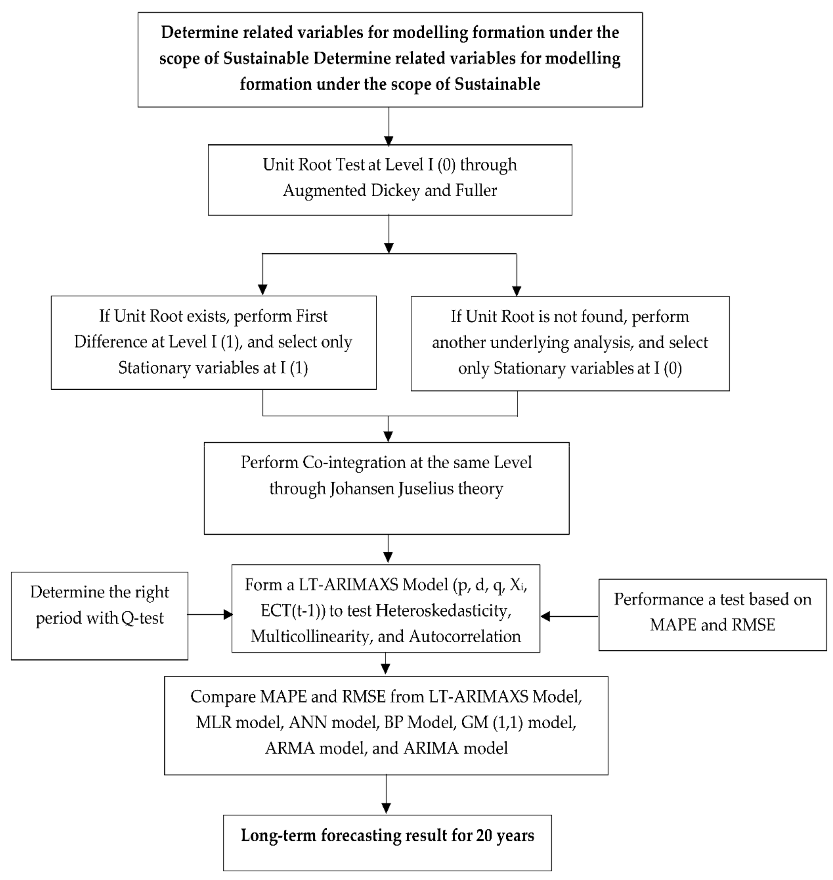
Hence, we considered the above gap as an important issue that has to be addressed. Simultaneously, we developed a forecasting model for final energy consumption by adapting various theoretical concepts, conceptual frameworks, research, variable selection, and the implementation of the heteroskedasticity test, multicollinearity test, and autocorrelation for spurious check. Additionally, the co-integration model was optimized by incorporating an error correction mechanism test to differentiate this model from the other existing models. This newly developed model comes under the name of the Long Term-Autoregressive Integrated Moving Average with Exogeneous variables and Error Correction Mechanism model (LT-ARIMAXS model). However, we developed the LT-ARIMAXS model to differentiate from other models and to fill the recent gap existing in old models that was found in the research review. The existing models include the MLR model, ANN model, BP model, GM(1,1) model, ARMA model, and ARIMA model, among others. The LT-ARIMAXS model is a forecasting model that aims to create an effectiveness in long-term forecasting to support long-term policy planning. Hence, the findings of this study become useful and applicable in both Thailand’s context and other contexts. The research’s flow chart is illustrated in Figure 1 and determines all the relevant variables for the final energy consumption forecasting model, whose characteristics fall under the long-term sustainable development policy of 20 years (2018–2037), with the Augment Dickey Fuller theory only at the same level by using data from 1985 to 2017. Moreover, only crucial and influential variables are used in the forecasting model.

The remainder of this paper is as follows: Section 2 discusses the materials and methods. Section 3 shows the results. Section 4 summarizes the discussion. Section 5 presents the conclusion.

2. Materials and Methods

2.1. Autoregressive Model and Moving Average Model

The autoregressive model and moving average model or Box–Jenkins are two models that emphasize only the stationary data [32,33], described as follows.

In the case of the random seasonal process, it is an uncertain or specific seasonal process. For instance, a country encounters a political conflict for the past many years. At the same time, a demonstration occurs at the second quarter. This situation causes a sales drop. However, the political conflicts may seem stable this year in the same quarter. Thus, the sale is consistent. Here, the seasonal process that took place last year at the second quarter temporarily affects this year’s second quarter, which can be called the stationary seasonal process. In this case, it is not necessary to drop off the season, but it can be incorporated into the model. This can be called the seasonal autoregressive moving average or (seasonal ARMA). The model is explained as below [34,35]:

$X_t$ is a quarter time series and falls under a stationary seasonal process. This time series $X_t$ can be written as:

$$X_t=A_1{X}_{t-4}+v_{{}_t},\left|A_1\right|<1$$

(1)

where $v_t$ is a random error variable, which is a white noise. The above equation is a AR(4) model where the coefficient of $X_{t-1},$ $X_{t-2}$ and $X_{t-3}$ is 0, and $\left|A_1\right|<1$ is the condition indicating the stationary seasonal process in time series $X_t$. If this $X_t$ is brought to find an average value, a variance of the Theoretical Autocorrelation Function (TAC) and Theoretical Partial Autocorrelation Function (TPAC) is computed through the following equation:

Let $\mu =0$, Variance ${\gamma }_0=\frac{{\sigma }^2}{1-A_1^2}$, the TAC is pointed in Equation (2) and TPAC is drawn in Equation (3).

$${\rho }_k=\{\begin{array}{c}{(A_1)}^{\frac{k}{4}},\\ 0,\end{array}k=0,4,8,...\text{when it is other case}$$

(2)

$${\varphi }_{kk}=\{\begin{array}{c}{\rho }_4\\ 0,\end{array}k=4\text{when it is other case}$$

(3)

Since $\left|A_1\right|<1$, when considering Equation (2), it can be concluded that, if $0<A_1<1$, TAC will exponentially reduce at time 4, 8, 12, …; if, as time slowly passes, TAC will be exponentially up and down at time 4, 8, 12, …; if $\left|A_1\right|$ is closely approaching 1, a seasonal pattern will be clearer and last longer; and if $\left|A_1\right|$ is close to 0, the pattern will disappear. Equation (3) shows that the TPAC is not equivalent to 0.

Based on Equation (1), it reflects only on the impact of season in AR, but the time series can be as the ARMA in practice, and this can be written as below:

$$A(L^s)X_t=B(L^s)v_t$$

(4)

where s is the time duration of season.

$$A(L^s)=1-A_1{L}^s-A_2{L}^{2s}-\dots A_p{L}^{ps}$$

(5)

$$B(L^s)=1-B_1{L}^s-B_2{L}^{2s}-\dots B_Q{L}^{Qs}$$

(6)

We consider Equation (4) as the pure seasonal $ARMA$ model at ${(P,Q)}_s$. In practice, it is possible that $X_t^{}$ is in AR(1), together influencing the season as the equation below:

$$X_t^{}=A_1{X}_{t-1}+A_1{X}_{t-4}+v_t,\left|{\alpha }_1\right|<1\mathrm{and}\left|A_1\right|<1$$

(7)

Equation (7) indicates the influence of seasonal process when $s=4$, and time series $X_t^{}$ in quarter 2 is related to quarter 1, while quarter 2 of this year is related to quarter 2 last year.

Meanwhile, Equation (4) shows $X_t^{}$ in some seasons of the $ARMA$ model at ${(P,Q)}_s$ or $ARMA$ $(p,q)$ together, and $v_t^{}$ in $ARMA$ $(p,q)$ is as follows:

$$v_t=\frac{\beta (L)}{\alpha (L)}{\epsilon }_t$$

(8)

where ${\epsilon }_t$ is the random error variable with white noise $\alpha (L)=1-{\alpha }_{1}L-{\alpha }_2{L}^2-\dots {\alpha }_p{L}^p$ and $\beta (L)=1-{\beta }_{1}L-{\beta }_2{L}^2-\dots {\beta }_q{L}^q$. Therefore, Equation (4) can be drawn as below:

$$A(L^s)\alpha (L)X_t=B(L^s)\beta (L){\epsilon }_t$$

(9)

Equation (9) is called the multiplicative seasonal $ARMA$ model at $(p,q)\times {(P,Q)}_s$, and can be denoted as $ARMA$ $(p,q){(P,Q)}_s$ or $ARMA$ $(p,q)\times {(P,Q)}_s$.

2.2. LT-ARIMAXS Model

In the construction of the LT-ARIMAXS model for forecasting, the autoregressive model (AR) and moving average model (MA) were basically integrated to first structure an ARIMA model. Once the ARIMA model was obtained, it was then applied to generate the LT-ARIMAXS model together with a co-integration test at the same level for every variable in the equations. In addition, there was also an adaptation of an error correction mechanism test in this particular model, as discussed below.

2.2.1. A Forecasting Model with ARIMA Model

It is a notion that differentiating at d with a particular time series will make a non-stationary time series a stationary time series. With such differentiation applied in the Box–Jenkins model, it can become known as $ARIMA(p,d,q)$ [34,35].

For better understanding, $X_t$ is denoted as the non-stationary time series, where $Z_t=\Delta X_t=X_t-X_{t-1}$ is the stationary time series. Here, a proper model for this time series $X_t$ is $ARIMA(1,1,0)$ and it can be written as:

$$Z_t={\alpha }_0+{\alpha }_1^{}{Z}_{t-1}+{\epsilon }_t\mathrm{where}t=1,2,\dots ,T$$

(10)

If time at $T$ is taken into account, the $ARIMA(1,1,0)$ becomes:

$$Z_T={\alpha }_0+{\alpha }_1^{}{Z}_{T-1}+{\epsilon }_T$$

(11)

and $X_1,X_2,\dots X_T$ (or denoted as $I_T$) is now known for their value.

When using Equation (11), we forecast ${\widehat{Z}}_{T+1},{\widehat{Z}}_{T+2},{\widehat{Z}}_{T+3}$ from the following equation.

$$\begin{array}{cccc}\begin{array}{cc}{\widehat{Z}}_{T+1}& =\end{array}& {\alpha }_0& +& {\alpha }_1\Delta X_T\\ \begin{array}{cc}{\widehat{Z}}_{T+2}& =\end{array}& {\alpha }_0& +& {\alpha }_1\Delta {\stackrel{\wedge }{X}}_{T+1}\\ \begin{array}{cc}{\widehat{Z}}_{T+3}& =\end{array}& {\alpha }_0& +& {\alpha }_1\Delta {\stackrel{\wedge }{X}}_{T+2}\\ \begin{array}{c}\begin{array}{cc}& \end{array}\\ \begin{array}{cc}{\widehat{Z}}_{T+j}& =\end{array}\end{array}& \begin{array}{c}⋮\\ {\alpha }_0\end{array}& \begin{array}{c}\\ +\end{array}& \begin{array}{c}\\ {\alpha }_1\Delta {\stackrel{\wedge }{X}}_{T+(j-1)}\end{array}\end{array}\}$$

(12)

From Equation (12), it can be seen that ${\widehat{X}}_T$ may not need forecasting. This is because the true information is known, which is $X_T$; hence, the forecasting result of ${\widehat{X}}_{T+1}$ can be computed from.

$${\widehat{X}}_{T+1}=X_T+{\widehat{Z}}_{T+1}$$

(13)

while the forecasting result of ${\widehat{X}}_{T+2},{\widehat{X}}_{T+3},\dots ,{\widehat{X}}_{T+j}$ can be calculated as follows:

$${\widehat{X}}_{T+j}=X_T+{\displaystyle \sum _{k=1}^j{\widehat{Z}}_{T+k}}$$

(14)

As for forecasting with $ARIMA(p,1,q)$, it can be applied by Equation (14), but the equation transformation is complicated.

Assuming the $ARIMA(p,1,q)$ model is written as below:

$$\begin{array}{l}{X}_t={\phi }_0+{\phi }_1{X}_{t-1}+{\phi }_2{X}_{t-2}+{\phi }_3{X}_{t-3}+\dots +{\phi }_p{X}_{t-p}\\ +{\phi }_{p+1}{X}_{t-p-1}+{\epsilon }_t-{\beta }_1{\epsilon }_{t-1}-{\beta }_2{\epsilon }_{t-2}-\dots -{\beta }_1{\epsilon }_{t-q}\end{array}$$

(15)

where ${\phi }_0={\alpha }_{0,}{\phi }_1={\alpha }_1+1,{\phi }_j={\alpha }_j-{\alpha }_{j-1}$ and ${\phi }_{p+1}=-{\alpha }_p$.

When the ARIMA model is obtained, it can then be used to construct the LT-ARIMAXS model. The construction is explained below.

2.2.2. A Forecasting Model with LT-ARIMAXS Model

For the LT-ARIMAXS model, we have adapted the concept from the basic models including ARIMA models [32,33], co-integration and error correction mechanism model [36,37]. This LT-ARIMAXS model was examined for the unit root test and variable selection for stationary into this model formation. We have determined the Level (I(0)) or first difference (I(1)) to analyze co-integration [36]. This point of analysis must reflect the relationship at the same level. However, this LT-ARIMAXS model must consist of the co-integration and error correction mechanism test (ECT) [37] to increase efficiency and the zero error in the model. In addition, the LT-ARIMAXS model comes with the suitability of future application in different areas in line with the policy of a particular country. This is due to the difference of the LT-ARIMAXS model with other models so that the ARIMA model focuses on the variables of Autoregressive (AR), Integrated (I), and Moving Average (MA) only at time t − i especially in past data. In this paper, the LT-ARIMAXS model differs from other old models due to the emphasis of Exogeneous Variables (${\displaystyle {\sum }_{i=1}^p{Y}_{t-i}}$), which is believed to be an important yet appropriate variable in the study. As for the reason, it is the influential variable that can affect the dependent variable. Additionally, the LT-ARIMAXS model uses Autoregressive (AR), Integrated (I), and Moving Average (MA) during time t − i in the study’s model. The LT-ARIMAXS model utilizes the co-integration and error correction mechanism test from the theory of Johansen and Juselius to increase the effectiveness of the model [36,37]. The co-integration model and error correction mechanism model can be explained below.

This model applies the Johansen co-integration test to examine a pattern called multivariate co-integration, which is the method proposed by Johansen and Juselius [36]; it is used to examine the long-term relationship between the variables. The essence of cointegration is that the linear combination of variables is stationary. Cointegration tests also require that all variables are integrated in the same order [37]. We can use the following formula to conduct the cointegration test.

$$X_t={\alpha }_0+{\displaystyle \sum _{i=1}^p{\alpha }_i}{X}_{t-i}+{\epsilon }_t$$

(16)

where $X_t$ is a (n × 1) vector of variables, ${\alpha }_0$ is a vector of constants, ${\alpha }_i$ is a (n × n) matrix of parameters, and ${\epsilon }_t$ is a (n × 1) vector of error term. Subtracting $X_{t-1}$ from each side of Equation (16) and letting I be an (n × n) identity matrix, it can be rewritten as follows.

$$\Delta X_t={\alpha }_0+\pi X_{t-1}+{\displaystyle \sum _{i=1}^p{\prod }_i}\Delta X_{t-i}+{\epsilon }_t$$

(17)

where ${\prod }_i$ and $\pi$ are the coefficient matrix and $\pi X_{t-1}$ is the error correction term, while the coefficient matrix $\pi$ provides information about the long term relationships among the variables. The number of the co-integration vectors can be determined by using the trace test and maximum eigenvalue test suggested by Johansen [37], as demonstrated in Equation (18) and (19).

$${\lambda }_{trace}=-T{\displaystyle \sum _{i=r+1}^n\ln (1-{\widehat{\lambda }}_1)}$$

(18)

$${\lambda }_{\max }(r,r+1)=-T{\displaystyle \sum _{i=r+1}^n\ln (1-{\widehat{\lambda }}_{r+1})}$$

(19)

where T is the sample size and $\lambda$ is the eigenvalue. Based on Equations (17) and (18), if the null hypothesis is rejected, it shows the testing variables consist of co-integration. On the other hand, if the null hypothesis is accepted, there is no co-integration.

After performing co-integration test, another important test must be carried out, which is error correction mechanism test [37]. We can find that the change of $X_t$ not only depends on the change of $Y_t$ but also depends on the change of the last period $Y_{t-1}$ and $X_{t-1}$. Considering the non-stationarity, the OLS test cannot be used to perform the regression. Therefore, Equation (32) can deform to the equation below.

$$\Delta X_t={\beta }_1\Delta Y_t-(1-\delta )(X_{t-1}-\frac{{\beta }_0}{1-\delta }-\frac{{\beta }_1+{\beta }_2}{1-\delta }{Y}_{t-1})+{\epsilon }_t$$

(20)

Hence, the LT-ARIMAXS model can be written below.

$$\begin{array}{l}{X}_t={\phi }_0+{\phi }_1{X}_{t-1}+{\phi }_2{X}_{t-2}+{\phi }_3{X}_{t-3}+\dots +{\phi }_p{X}_{t-p}\\ +{\phi }_{p+1}{X}_{t-p-1}+{\epsilon }_t-{\beta }_1{\epsilon }_{t-1}-{\beta }_2{\epsilon }_{t-2}-\dots -{\beta }_1{\epsilon }_{t-q}\\ +{\displaystyle \sum _{i=1}^p{Y}_{t-i}+}{\displaystyle \sum _{i=1}^{p}EC{T}_{t-i}}\end{array}$$

(21)

Let ${\phi }_0={\alpha }_0,{\phi }_1={\alpha }_1+1,{\phi }_j={\alpha }_{j-1},{\phi }_{p+1}=-{\alpha }_p$, ${\displaystyle \sum _{i=1}^p{Y}_{t-i}}$ = exogeneous variables, which are stationary at the level and ${\displaystyle \sum _{i=1}^{p}EC{T}_{t-i}}$ = the error correction mechanism test.

Equation (21) indicates the components of the LT-ARIMAXS model comprised of: (1) Autoregressive variables (AR); (2) Moving Average (MA); (3) exogenous variables (); and (4) error correction mechanism ${\displaystyle \sum _{i=1}^{p}EC{T}_{t-i}}$. The LT-ARIMAXS model is built and developed with the assurance of being Heteroskedasticity, Multicollinearity, and Autocorrelation free. There is also an analysis of period identification with the Q-statistics test as to ensure that the model is not spurious while it becomes efficient in the forecasting with fewer errors. The model is then able to be applied in a different context and management policy.

2.2.3. Measurement of the Forecasting Performance

To evaluate the forecasting effect of each model, we employed the mean absolute percentage error (MAPE) and the root mean square error (RMSE) to compare the forecasting accuracy of each model. The calculated equations are shown below [35,38].

$$\mathrm{MAPE}=\frac{1}{n}{\displaystyle \sum _{i=1}^n\left|\frac{{\widehat{y}}_i-y_i}{y_i}\right|}$$

(22)

$$\mathrm{RMSE}=\sqrt{\frac{1}{n}{\displaystyle \sum _{i=1}^n{\left({\widehat{y}}_i-y_i\right)}^2}}$$

(23)

The LT-ARIMAXS model is a newly developed method completed by adapting various concepts from the general models including autoregressive (AR), integrate (I), and moving average (MA). For the variable selection criterion, the variables must only be causal factors or stationary at the same level. The stationary level I(0) or first difference I(1) are used to test the unit root test. With the right variables, we fulfill the criterion. Those variables are put forth for a co-integration test. When they are found to be co-integrated, they are then used in structuring the LT-ARIMAXS model (p, d, q, Xi, ECT_(t−1)) with an appropriateness check of period (t − i) through the implementation of a white noise process by the Q test statistic method. In this paper, the LT-ARIMAXS model (p, d, q, Xi, ECT_(t−1)) must not be free from heteroskedasticity, multicollinearity, and autocorrelation. Testing the LT-ARIMAXS model (p, d, q, Xi, ECT_(t−1)) can be done based with MAPE and RMSE, and comparing those two values with existing models. Once the model is obtained, forecasting the future is the next essential step. We have combined the dataset using Microsoft Office Excel. In addition, EViews 9.5 software is deployed to implement the model, and it flows as below.

(1)

Place the stationary variables at the same level in the analysis of the long-term relationship based on the Johansen and Juselius concept.

(2)

Create a forecasting model by adapting the advance statistics of the so-called LT-ARIMAXS model with full consideration of the relationship of all causal variables in terms of both the error correction mechanism test and the co-integration test.

(3)

Examine the goodness of fit in two aspects: (1) appropriateness check of period (t − i) through the implementation of a white noise process by the Q test statistic method; and (2) performance test for the LT-ARIMAXS model based on MAPE and RMSE. Compare those two values derived from the LT-ARIMAXS model with the existing model, including MLR model, the ANN model, BP Model, GM(1,1) model, ARMA model, and ARIMA model.

(4)

Forecast final energy consumption by using the LT-ARIMAXS model for the period from 2018 to 2037, totaling 20 years. The flowchart of the LT-ARIMAXS model is shown in Figure 1.

3. Results

3.1. Screening of Influencing Factors for Model Input

We tested the factors in the context of Thailand’s sustainable development policy. Here, we deployed the time series data of the period 1987–2017. The tested factors consisted of eight variables, namely final energy consumption ($\ln \left(\mathrm{EC}\right)$), per capita GDP ($\ln \left(\mathrm{GDP}\right)$), population growth ($\ln \left(\mathrm{Population}\right)$), oil price ($\ln \left(\mathrm{OP}\right)$), energy intensity ($\ln \left(\mathrm{EI}\right)$), urbanization rate ($\ln \left(\mathrm{UG}\right)$), industrial structure ($\ln \left(\mathrm{IS}\right)$), and net exports ($\ln (\mathrm{X}-\mathrm{E})$). The test was conducted based on the Augment Dickey Fuller theory at Level I(0) and first difference I(1), as illustrated in

Table 1. Unit root test at Level I(0) and First Difference I(1).

ADF Test at Level I(0)		ADF Test at First Difference I(1)		MacKinnon Critical Value
Variables	Value	Variables	Value	1%	5%	10%
$\ln \left(\mathrm{EC}\right)$	−2.85	$\Delta \ln \left(\mathrm{EC}\right)$	−4.56 ***	−4.22	−3.53	−3.20
$\ln \left(\mathrm{GDP}\right)$	−2.24	$\Delta \ln \left(\mathrm{GDP}\right)$	−5.26 ***	−4.22	−3.53	−3.20
$\ln \left(\mathrm{Population}\right)$	−2.75	$\Delta \ln \left(\mathrm{Population}\right)$	−4.25 ***	−4.22	−3.53	−3.20
$\ln \left(\mathrm{OP}\right)$	−3.05	$\Delta \ln \left(\mathrm{OP}\right)$	−5.11 ***	−4.22	−3.53	−3.20
$\ln \left(\mathrm{EI}\right)$	−3.11	$\Delta \ln \left(\mathrm{EI}\right)$	−4.95 ***	−4.22	−3.53	−3.20
$\ln \left(\mathrm{UG}\right)$	−2.39	$\Delta \ln \left(\mathrm{UG}\right)$	−4.77 ***	−4.22	−3.53	−3.20
$\ln \left(\mathrm{IS}\right)$	−3.12	$\Delta \ln \left(\mathrm{IS}\right)$	−5.71 ***	−4.22	−3.53	−3.20
$\ln (\mathrm{X}-\mathrm{E})$	−3.60	$\Delta \ln (\mathrm{X}-\mathrm{E})$	−4.78 ***	−4.22	−3.53	−3.20

Note: $\mathrm{EC}$ is the final energy consumption; $\mathrm{GDP}$ is the per capita GDP; $\mathrm{Population}$ is the population growth; $\mathrm{OP}$ is the oil price; $\mathrm{EI}$ is the energy intensity; $\mathrm{UG}$ is the urbanization rate; $\mathrm{IS}$ is the industrial structure; $\mathrm{X}-\mathrm{E}$ is the net export, *** denotes a significance, α = 0.01, compared to the Tau test with the MacKinnon Critical Value, $\Delta$ is the first difference, and $\ln$ is the natural logarithm.

.

Table 1 presents the testing result of the Tau test compared to the MacKinnon critical value. The result showed that all variables had the unit root or were found to be non-stationary at Level I(0), and explained the insignificance at 1%, 5%, and 10%. Therefore, carrying out the First Difference I(1) was required. When testing the unit root at Level I(1), it was found that all variables were stationary at Level I(1) with the significance level of 1%, 5%, and 10%. Later, all stationary variables are taken for the co-integration test by Johansen Juselius to analyze the long-term relationship of every variable at the same level as shown in

Table 2. Co-integration test by Johansen Juselius.

Variables	Hypothesized No of CE(S)	Trace Statistic Test	Max-Eigen Statistic Test	MacKinnon Critical Value		Status
				1%	5%
$\Delta \ln \left(\mathrm{EC}\right)$,$\Delta \ln \left(\mathrm{GDP}\right)$, $\Delta \ln \left(\mathrm{Population}\right)$, $\Delta \ln \left(\mathrm{OP}\right)$, $\Delta \ln \left(\mathrm{EI}\right)$,$\Delta \ln \left(\mathrm{UG}\right)$,$\Delta \ln \left(\mathrm{IS}\right)$$\Delta \ln (\mathrm{X}-\mathrm{E})$	None ***	231.15	165.85	18.75	15.40	I(1)
	At Most 1 ***	79.41	81.45	5.50	3.12	I(1)

*** denotes significance α = 0.01.

.

3.2. Analysis of Co-Integration

Table 2 shows that all variables had a long-term relationship (co-integration) because the results of the trace test were 231.15 and 79.41, which were higher than the MacKinnon critical values at significance levels of 1% and 5%. The maximum eigenvalue test results were 165.85 and 81.45, which were higher than the MacKinnon critical values at the same significance levels. Consequently, those variables were used to form a forecasting model by adapting the LT-ARIMAXS model and applying short- and long-term relationships into the model.

3.3. Formation of Analysis Modeling with the LT-ARIMAXS Model

All stationary variables at the first difference are tested for the co-integration at the same level to construct the LT-ARIMAXS Model at time (1,1,1). All exogenous variables at time t − 1 and ECT(t − 1) are not proper as evaluated by the Q-statistic. However, we have started to build the Best model named as the LT-ARIMAXS model at period (t − i) of p,d,q, and the good fit of period (t − i) falls at LT-ARIMAXS (2,1,2), which is shown in Figure 2 and

Table 3. The result of the LT-ARIMAXS model (2,1,2).

Independent Variables	Dependent Variable $\Delta {\mathbf{ln}\left(\mathbf{EC}\right)}_{\mathit{t}}$
$\mathrm{A}\mathrm{R}(1)$	2.79 ***
$\mathrm{A}\mathrm{R}(2)$	3.15 ***
$\mathrm{M}\mathrm{A}(1)$	2.99 ***
$\mathrm{M}\mathrm{A}(2)$	2.41 **
$\Delta {\ln \left(\mathrm{GDP}\right)}_{t-1}$	7.06 ***
$\Delta {\ln \left(\mathrm{Population}\right)}_{t-1}$	2.45 **
$\Delta {\ln \left(\mathrm{OP}\right)}_{t-2}$	6.15 ***
$\Delta {\ln \left(\mathrm{EI}\right)}_{t-1}$	3.42 ***
$\Delta {\ln \left(\mathrm{UG}\right)}_{t-1}$	5.26 ***
$\Delta {\ln \left(\mathrm{IS}\right)}_{t-1}$	7.34 ***
$\Delta \ln (\mathrm{X}-{\mathrm{E})}_{t-2}$	5.01 ***
${\mathrm{ECT}}_{t-1}$	−2.15 **

Note: $\mathrm{A}\mathrm{R}$ is Autoregressive model, $\mathrm{M}\mathrm{A}$ is Moving Average model, *** denotes significance α = 0.01, ** denotes significance α = 0.05, R-squared is 0.91, adjusted R-squared is 0.90, the Durbin–Watson statistic is 2.01, the F-statistic is 229.25 (probability is 0.00), the ARCH test is 35.01 (probability is 0.1), the LM test is 1.65 (probability is 0.10), and the response test (${\chi }^2>\mathrm{critical}$) represents the significance.

.

Figure 2 reflects that the LT-ARIMAXS (2,1,2) model became the best forecasting model as all values of the Q test statistic at time (t − i) were in the criteria and met all conditions, or the insignificance fell as follows: α = 0.01, α = 0.05, and α = 0.1. Therefore, this model can be used to forecast the final energy consumption. However, we have discovered the best model at time LT-ARIMAXS (2,1,2), and this allowed us to understand the influence in changes or elasticity of all independent variables causing the changes over the final energy consumption at time (t − i), as illustrated in Table 3.

Table 3 illustrates the parameters of the LT-ARIMAXS (2,1,2) model at a statistically significant level of 1% and 5%. The findings illustrated that, when per capita GDP ($\Delta {\ln \left(\mathrm{GDP}\right)}_{t-1}$at time (t − 1) changed about 1%, it changed the final energy consumption ($\Delta {\ln \left(\mathrm{EC}\right)}_t$) equivalent to the elasticity coefficient of 7.06% at the significance level of 1%, which went in the same direction. When population growth ($\Delta {\ln \left(\mathrm{Population}\right)}_{t-1}$at time (t − 1) changed about 1%, it showed influence over the final energy consumption ($\Delta {\ln \left(\mathrm{EC}\right)}_t$) equivalent to the elasticity coefficient of 2.45% at the significance level of 5%, which also went in the same direction. When oil price ($\Delta {\ln \left(\mathrm{OP}\right)}_{t-2}$) at time (t − 2) changed about 1%, the final energy consumption ($\Delta {\ln \left(\mathrm{EC}\right)}_t$) was affected to change by the elasticity coefficient of 6.15% at the significance level of 1%, whose change was in the same direction. When energy intensity ($\Delta {\ln \left(\mathrm{EI}\right)}_{t-1}$) at time (t − 1) changed about 1%, the final energy consumption ($\Delta {\ln \left(\mathrm{EC}\right)}_t$) was also changed by the elasticity coefficient of 3.42% at the significance level of 1%, which went in the same direction. When the change in urbanization rate (${\ln \left(\mathrm{UG}\right)}_{t-1}$) at time (t − 1) accounted for 1%, the final energy consumption ($\Delta {\ln \left(\mathrm{EC}\right)}_t$) was also affected to change by the elasticity coefficient of 5.26% at the significance level of 1%, which went in the same direction. When industrial structure (${\ln \left(\mathrm{IS}\right)}_{t-1}$) at time (t − 1) changed about 1%, it affected the final energy consumption ($\Delta {\ln \left(\mathrm{EC}\right)}_t$) equivalent to the elasticity coefficient of 7.34% at the significance level of 1%, whose direction went in the same direction. Furthermore, when net exports ($\ln (\mathrm{X}-{\mathrm{E})}_{t-2}$) at time (t − 2) changed about 1%, the final energy consumption ($\Delta {\ln \left(\mathrm{EC}\right)}_t$) was changed equally with the elasticity coefficient of 5.01% at the significance level of 1% in the same direction.

However, from the analysis of the LT-ARIMAXS model (2,12), it was found that ${\mathrm{ECT}}_{t-1}$ was equal to −2.15% at the significance level of 5%. This shows that the error-correction mechanism (${\mathrm{ECT}}_{t-i}$) can precisely explain the fluctuations and the adjustment. Specifically, ${\mathrm{ECT}}_{t-1}$ denotes that, under the impacts of controlled variables, when short-term fluctuations deviate from the long-term equilibrium, the changes of final energy consumption in t time can eliminate the non-equilibrium error of the t − 1 time by 2.15% and make a reverse adjustment to bring the non-equilibrium point back to the equilibrium point. Furthermore, the LT-ARIMAXS model (2,1,2) is free from the issue of heteroskedasticity, multicollinearity, and autocorrelation.

In addition, we compared some selected forecasting models in terms of their effectiveness with MAPE and RMSE, which is indicated in

Table 4. The performance monitoring of the forecasting model (%).

Forecasting Model	MAPE	RMSE
MLR model	19.76	20.76
BP model	10.67	14.63
ANN model	8.55	9.95
ARMA model	8.51	9.17
GM(1,1) model	6.69	8.52
ARIMA model	5.75	6.41
LT-ARIMAXS model (2,1,2)	0.97	2.12

. LT-ARIMAXS model was compared with other models: the MLR model, the BP model, the ANN model, the ARMA model, the GM(1,1) model, and the ARIMA model shown below.

Table 4 shows that LT-ARIMAXS model (2,1,2) with analytical data for 1985–2017 consisting of independent variables in the model including final energy consumption at the time period t − 1 (${\ln \left(\mathrm{EC}\right)}_{t-1}$) or AR(1), final energy consumption at time period t − 2 (${\ln \left(\mathrm{EC}\right)}_{t-2}$) or AR(2), Moving Average (1) or MA(1), Moving Average (2) or MA(2), per capita GDP at time period t − 1 (${\ln \left(\mathrm{GDP}\right)}_{t-1}$), population growth at time period t − 1 (${\ln \left(\mathrm{Population}\right)}_{t-1}$),oil price at time period t − 2 (${\ln \left(\mathrm{OP}\right)}_{t-2}$), energy intensity at time period t − 1 (${\ln \left(\mathrm{EI}\right)}_{t-1}$), urbanization rate at time period t − 1 (${\ln \left(\mathrm{UG}\right)}_{t-1}$), industrial structure at time period t − 1 (${\ln \left(\mathrm{IS}\right)}_{t-1}$), net exports at time period t − 2 ($\ln (\mathrm{X}-{\mathrm{E})}_{t-2}$), and the error-correction mechanism at time period t − 1 (${\mathrm{ECT}}_{t-1}$) provided the lowest MAPE value at 0.97% and RMSE value at 2.12%. The ARIMA model, the GM(1,1) model, the ARMA model, the ANN model, the BP model, and the MLR model had MAPE values of 5.75%, 6.69%, 8.51%, 8.55%, 10.67%, and 19.76%, respectively, and RMSE values of 6.41%, 8.52%, 9.17, 9.95%, 14.63%, and 20.76%, respectively. The findings show that the LT-ARIMAXS model (2,1,2) is most effective. This was observed as MAPE and RMSE being the lowest when compared to the old models. Furthermore, it is very useful for long-term forecasting and national policy-making and planning in boosting sustainable development in the long-run. Therefore, the LT-ARIMAXS model (2,1,2) was used to forecast CO₂ emissions in the following step.

3.4. Final Energy Consumption Forecasting Based on the LT-ARIMAXS Model

Table 4 shows that the LT-ARIMAXS Model comes with highest efficiency by looking at the lowest value of MAPE and RMSE compared with past forecasting models. Therefore, we chose the LT-ARIMAXS Model for long-term forecasting (2018–2037). Once we attained the best model, i.e., the LT-ARIMAXS Model (2,1,2), the long-term forecasting on the final energy consumption in Thailand’s petroleum industries sector for 20 years (2018–2037) was conducted, as shown in Figure 3.

Figure 3 shows that final energy consumption from 2018 to 2037 in Thailand constantly increases where the 2037 rate was found to be 109.8% higher than 2017. At the same time, it presents that the 2037 final energy consumption would be equivalent to 121,461 ktoe, which is higher than the government’s reduction goal, i.e., the final energy consumption in Thailand’s petroleum industries sector should not exceed more than 90,000 ktoe. As for the study, it reflects that the final energy consumption does not go along with the national policy effectively, and has negative effects on Thailand’s sustainable development in the long-run.

4. Discussion

This research differs from other previous studies, as this LT-ARIMAXS model has a higher effectiveness and better long-term forecasting, while producing fewer discrepancies in prediction. Based on the many relevant studies reviewed, most existing models were only made available for short-term forecasting capability ranging from one to five years. Zhao, Zhao, and Guo [6] applied the GM model optimized by MFO with rolling mechanism in the forecasting for the period 2010–2014. Li and Li [7] used the ARIMA model, GM model, and ARIMA-GM model to forecast energy consumption in Shandong, China from 2016 until 2020. Xiong, Dang, Yao, and Wang [8] utilized the GM(1,1) model based on optimizing the initial condition in accordance with the new information priority principle in the prediction from 2013 to 2017. Panklib, Prakasvudhisarn and Khummongkol [9] chose ANN model and MLR model in the forecasting for 2010, 2015, and 2020. In addition, Azadeh, Ghaderi, Tarverdian, and Saberi [10] incorporated ANN integrated with the genetic algorithm in a one-year prediction. Günay [11] implemented Artificial Neural Networks using predicted values of socio-economic indicators and climatic conditions for the same one-year coverage of forecasting. Dai, Niu, and Li [12] applied ensemble empirical mode decomposition and least squares support vector machine based on an improved shuffled frog leaping algorithm for 2018–2022 forecasting. Suganthi and Samuel [14] used the econometrics model for 2030–2031 forecasting. Additionally, there have also been some studies that have attempted to forecast for six years but not 20 years. Hamzacebi and Es [18] implemented an optimized Grey Modeling for 2013–2025 forecasting. Mu et al. [19] used improved grey model for the 2011–2020 prediction. Zeng, Zhou, and Zhang [20] developed a homologous grey prediction model for 2018–2024 forecasting. Furthermore, Jiang, Yang, and Li [21] used MGM model, ARIMA model, MGM–ARIMA model, and BP model for the forecasting period of 2017–2030. Ediger and Akar [22] deployed ARIMA model and SARIMA model for 2005–2020 forecasting. Ekonomou [23] applied ANN model for 2005–2008, 2010, 2012, and 2015 prediction. Seung et al. [26] also deployed a MLR model for 2014–2030 forecasting. Ayvaz and Kusakci [31] chose to apply a NDGM model in prediction for the period 2014–2030. However, by reviewing various studies, it was found that long-term forecasting has become a popular topic most researchers have chosen to study, and various different methodologies have been implemented. In this study, we selected the most appropriate model for long-term forecasting. The LT-ARIMAXS model functioned better and was more efficient, with less erro, when compared to other models. With the output of the model, it is very useful and fits in Thailand’s policy-making and planning. Furthermore, it can become the best guideline for any interested researchers to further develop and explore.

Nonetheless, the limitation of this research lies upon the diesel price as the government controls the price by using the Diesel Oil Support Fund. As a result, it does not reflect the real economy and energy demand due to this government intervention, which may result in inaccurate forecasting. If the government allows the oil price to move with the world market, we would be able to obtain the true influence of the diesel price over the change in final energy consumption. In addition, the government’s policy does not specifically define the government expenditure, especially on mega projects the government has invested in, which heavily effects the economy, society, and environment. If such variable can be utilized and considered in policy-making, we wouls also be able to see the influence affecting the change in energy consumption. However, we highly expect that the LT-ARIMAXS model is applied for a formulation of sustainable development-based policy and future research. In addition, it is used to forecast greenhouse gases as determined by Thailand in all terms of durations including short-term (1–5 years), mid-term (6–10 years), and long-term (11–20 year). However, the variables must be contributed as the causal factors, especially a global diesel price and government expenditure. Nonetheless, all factors are tested for the stationary, co-integration, and the error correction mechanism. Most importantly, these two factors of global diesel price and government expenditure are used in direct and indirect relationship analysis to ensure the real influence.

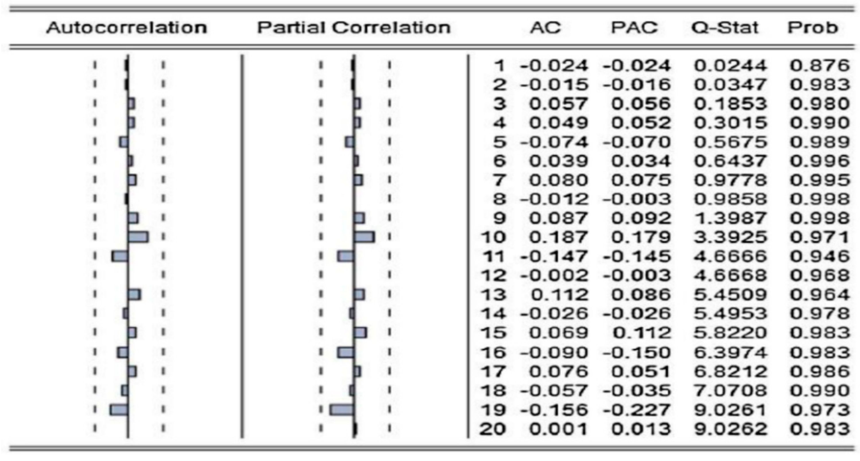
A government policy formulation requires a number of factors. Apart from variables used in this study, the other true influential factors must be considered. Those factors are those truly affecting the change in final energy consumption especially in long-term forecasting. The true and complete factors must be emphasized and applied in future policy-making since their characteristics qualify and fulfill the criterion as complete factors. Increasing the numbers of foreign tourists, the increment of foreign workers, and carbon emission intensity are some factors to consider. Since the existing models do not produce a precise output and are less efficient in forecasting, the LT-ARIMAXS model has, therefore, been designed to fill this gap. Additionally, the LT-ARIMAXS model is structured with detailed research methodology together with a fine selection of variables emphasizing on the influential factors over the changes in the final energy consumption. At the same time, both co-integration and an error correction mechanism test are carried out to ensure zero heteroscedasticity, multicollinearity, and autocorrelation. The proper period is specified based on the Q-statistic test for constructing the LT-ARIMAXS model (2,1,2). With all processes put together, the model is completely ready for long-term prediction (2018–2037) and analysis of MAPE and RMSE for further comparison with the MLR model, the BP model, the ANN model, the ARMA Model, the GM(1,1) model, and the ARIMA model. The study reflected that the LT-ARIMAXS model (2,1,2) has a higher effectiveness with less error based on the evaluation from MAPE and RMSE.

However, the LT-ARIMAXS model is unique in terms of its variables used, as only causal factors affecting future forecasting are considered. This means all irrelevant factors are removed from the modeling. This study is very instrumental not only for Thailand but also other countries. To ensure its structure, all variables are rightly deployed, according to the proper context by analyzing the co-integration and carrying out an error correction test together by specifying the right period for the right sectors. The LT-ARIMAXS model does not limit the casual factors, but the users must give details in all processes for a better performance of the model. We used various software for our analysis by collecting data via Excel and constructing the LT-ARIMAXS model with EViews 9.5 due to its capability in precise and long-term analysis and supportive to window (64 bit). Nonetheless, for those individuals interested in using the LT-ARIMAXS model, they can download the EViews 9.5 student version for Windows (Windows 10, Windows 8, Windows 7, and Windows Vista) for free, but it only allows free usage for two years. A Pentium or better CPU with 512 MB Memory and 270 MB Disk Space is required.

However, from this study, it can be concluded that the final energy consumption in the long-run (2018–2037) by using the LT-ARIMAXS model will be higher than the targeted amount. In addition, this model differs from any existing models used on the prediction within Thailand since the model’s prediction result can really support Thailand’s national policy-making at a higher efficiency. Since the LT-ARIMAXS model is developed, only true influential variables over the final energy consumption in particular sectors are deployed and become applicable at a wider scope of prediction compared to past predictions. If the government decides to utilize the LT-ARIMAXS model as part of obtaining sustainability, all influences produced from the LT-ARIMAXS model (2,1,2) must be considered to attain a proper management of changes in all casual factors. One of the major key variables in the LT-ARIMAXS model is the error-correction mechanism (ECT). This is because the implication of the model is very beneficial for a long-term prediction for Thailand and other countries. When there are changes, shocks, or variations in the variables deviating from the equilibrium, the ECT is the value telling that those variables will adjust to the equilibrium in the next period (t − i). However, the ECT parameter will indicate the capability range of the adaptation to the equilibrium and it will guide the government to set a clearer path in policy-planning. In addition, the focus in modeling should be emphasized while other untaken variables are used for consideration by specifying a proper period of application to maximize the model’s use.

5. Conclusions

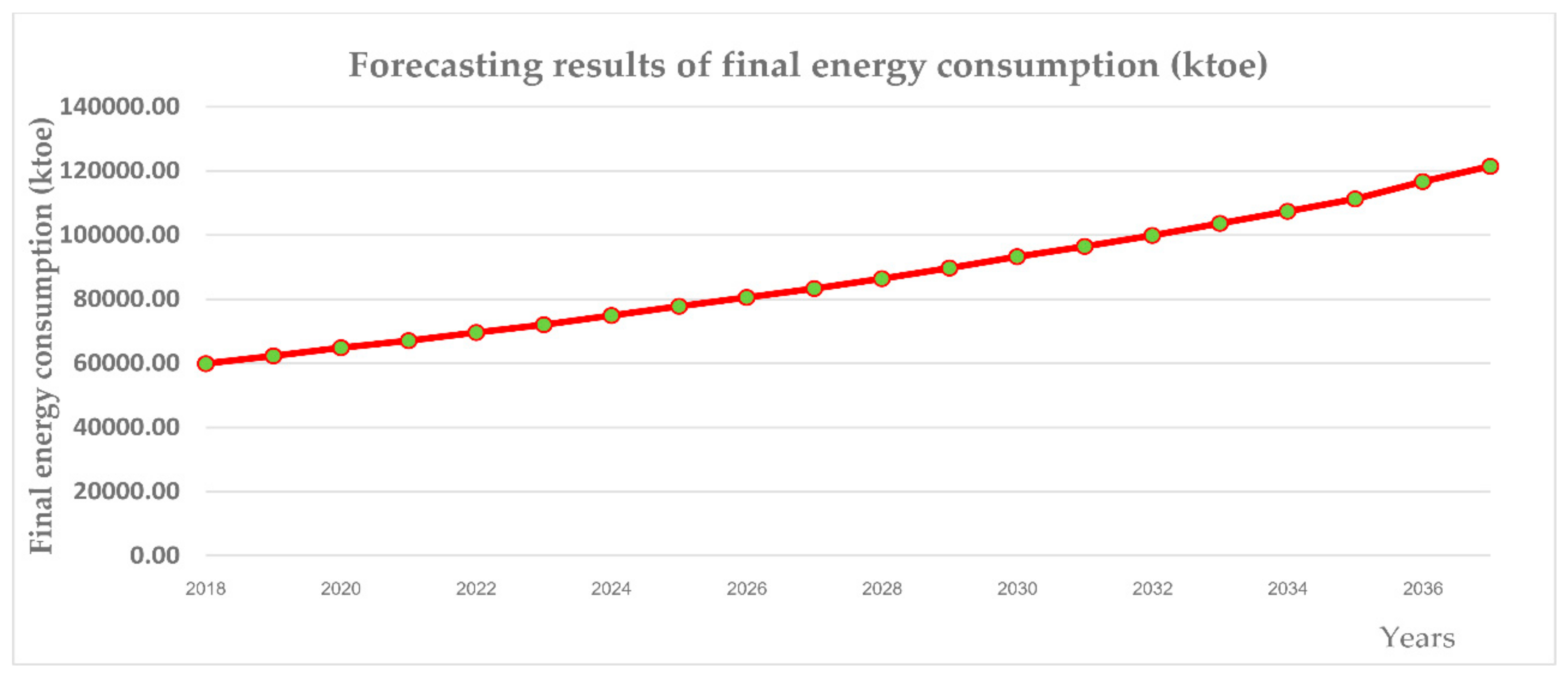
This study has formed another area to explore and acted as a guideline for future research. This has made the model standout from other past models. At the same time, it has helped to narrow the gap and strengthen the existing weaknesses in previous studies, reducing potential discrepancies. Therefore, this study was necessary as it is beneficial and instrumental for both academia and strengthening future sustainable development policy. This LT-ARIMAXS model has been structured based on previous models, and has become the first model to optimize the advance statistic. Simultaneously, it was designed to fill the gap of forecasting capability, especially long-term forecasting, which is important and necessary to develop to reduce any potential residual discrepancies. The reason for this assurance is that it allows us to improve policy formulation in the right direction in the most efficient and effective manner. We have developed this LT-ARIMAXS model by commencing with variable selection. This selection uses only influential variables, which have an impact on the change in final energy consumption, and must be felt within the sustainable development concept in both the long-term and short-term. When the right variables are obtained, they are used for the unit root test to identify the stationary at the same level. If any variables are found to be stationary yet at different levels, they are immediately eliminated. In this study, it was found that all involved variables were stationary at first difference, and they were used for the co-integration test to evaluate the long-term relationship. This test showed that all variables were co-integrated at Level I(1). After all those processes, the LT-ARIMAXS model (2,1,2) was structured consisting of the autoregressive model (AR), moving average model (MA), exogeneous variable, and error correction mechanism test (${\mathrm{ECT}}_{t-1}$). However, the LT-ARIMAXS model (2,1,2) was improved for the right period (t − i) as shown in the correlogram of the residual error with the use of the Q statistic test. With this test, we were able to identify the period for this modeling to be the most effective. In addition, we tested the effectiveness of the LT-ARIMAXS model (2,1,2) by MAPE and RMSE, whose values were later found to be lowest, equivalent to 0.97% and 2.12% when compared to the ARIMA model, GM(1,1) model, ARMA model, ANN model, BP model, and MLR model. Thus, the LT-ARIMAXS model (2,1,2) was used to forecast the final energy consumption in the petroleum industries sector in Thailand for 20 years (2018–2037). As a result, the model produced outcomes where the rate 2037 was 109.8% higher than 2017. Additionally, the final energy consumption was found to be 121,461 ktoe by 2037, and this exceeds the government limit of 90,000 ktoe. Hence, the above output can be applied in policy-making and planning in the future to ensure that the right policy for the right direction is established, unlike any other previous years (1985–2017).

References

1. Office of the National Economic and Social Development Board (NESDB). Available online: http://www.nesdb.go.th/nesdb_en/more_news.php?cid=154&filename=index (accessed on 27 June 2018).
2. National Statistic Office Ministry of Information and Communication Technology. Available online: http://web.nso.go.th/index.htm (accessed on 28 June 2018).
3. Department of Alternative Energy Development and Efficiency. Available online: http://www.dede.go.th/ewtadmin/ewt/dede_web/ewt_news.php?nid=47140 (accessed on 29 June 2018).
4. Achawangkul, Y. Thailand’s Alternative Energy Development Plan. Available online: http://www.unescap.org/sites/default/files/MoE%20_%20AE%20policies.pdf (accessed on 29 June 2018).
5. Thailand Greenhouse Gas Management Organization (Public Organization). Available online: http://www.tgo.or.th/2015/thai/content.php?s1=7&s2=16&sub3=sub3 (accessed on 29 June 2018).
6. Zhao, H.R.; Zhao, H.R.; Guo, S. Using GM(1,1) Optimized by MFO with Rolling Mechanism to Forecast the Electricity Consumption of Inner Mongolia. Appl. Sci. 2016, 6, 20. [Google Scholar] [CrossRef]
7. Li, S.; Li, R. Comparison of forecasting energy consumption in Shandong, China Using the ARIMA model, GM model, and ARIMA-GM model. Sustainability 2017, 9, 1181. [Google Scholar]
8. Xiong, P.P.; Dang, Y.G.; Yao, T.X.; Wang, Z.X. Optimal modeling and forecasting of the energy consumption and production in China. Energy 2014, 77, 623–634. [Google Scholar] [CrossRef]
9. Panklib, K.; Prakasvudhisarn, C.; Khummongkol, D. Electricity Consumption Forecasting in Thailand Using an Artificial Neural Network and Multiple Linear Regression. Energy Sources Part B Econ. Plan. Policy 2015, 10, 427–434. [Google Scholar] [CrossRef]
10. Azadeh, A.; Ghaderi, S.F.; Tarverdian, S.; Saberi, M. Integration of artificial neural networks and genetic algorithm to predict electrical energy consumption. Appl. Math. Comput. 2007, 186, 1731–1741. [Google Scholar] [CrossRef]
11. Günay, M.E. Forecasting annual gross electricity demand by artificial neural networks using predicted values of socio-economic indicators and climatic conditions: Case of Turkey. Energy Policy 2016, 90, 92–101. [Google Scholar] [CrossRef]
12. Dai, S.; Niu, D.; Li, Y. Forecasting of Energy Consumption in China Based on Ensemble Empirical Mode Decomposition and Least Squares Support Vector Machine Optimized by Improved Shuffled Frog Leaping Algorithm. Appl. Sci. 2018, 8, 678. [Google Scholar] [CrossRef]
13. Wang, Q.; Li, R. Decline in China’s coal consumption: An evidence of peak coal or a temporary blip? Energy Policy 2017, 108, 696–701. [Google Scholar] [CrossRef]
14. Suganthi, L.; Samuel, A.A. Modelling and forecasting energy consumption in INDIA: Influence of socioeconomic variables. Energy Sources Part B Econ. Plan. Policy 2016, 11, 404–411. [Google Scholar] [CrossRef]
15. Xu, J.; Fleiter, T.; Eichhammer, W.; Fan, Y. Energy consumption and CO2 emissions in China’s cement industry: A perspective from LMDI decomposition analysis. Energy Policy 2012, 50, 821–832. [Google Scholar] [CrossRef]
16. Kishita, Y.; Yamaguchi, Y.; Umeda, Y. Describing Long-Term Electricity Demand Scenarios in the Telecommunications Industry: A Case Study of Japan. Sustainability 2016, 8, 52. [Google Scholar] [CrossRef]
17. Zhao, W.; Wang, J.; Lu, H. Combining forecasts of electricity consumption in China with time-varying weights updated by a high-order Markov chain model. Omega 2014, 45, 80–91. [Google Scholar] [CrossRef]
18. Hamzacebi, C.; Es, H.A. Forecasting the annual electricity consumption of Turkey using an optimized grey model. Energy 2014, 70, 165–171. [Google Scholar] [CrossRef]
19. Mu, H.; Dong, X.; Wang, W.; Ning, Y.; Zhou, W. Improved Gray Forecast Models for China’s Energy Consumption and CO, Emission. J. Desert Res. 2002, 22, 142–149. [Google Scholar]
20. Zeng, B.; Zhou, M.; Zhang, J. Forecasting the Energy Consumption of China’s Manufacturing Using a Homologous Grey Prediction Model. Sustainability 2017, 9, 1975. [Google Scholar] [CrossRef]
21. Jiang, F.; Yang, X.; Li, S. Comparison of Forecasting India’s Energy Demand Using an MGM, ARIMA Model, MGM-ARIMA Model, and BP Neural Network Model. Sustainability 2018, 10, 2225. [Google Scholar] [CrossRef]
22. Ediger, V.S.; Akar, S. ARIMA forecasting of primary energy demand by fuel in Turkey. Energy Policy 2007, 35, 1701–1708. [Google Scholar] [CrossRef]
23. Ekonomou, L. Greek long-term energy consumption prediction using artificial neural networks. Energy 2010, 35, 512–517. [Google Scholar] [CrossRef] [Green Version]
24. Ardakani, F.J.; Ardehali, M.M. Long-term electrical energy consumption forecasting for developing and developed economies based on different optimized models and historical data types. Energy 2014, 65, 452–461. [Google Scholar] [CrossRef]
25. Supasa, T.; Hsiau, S.S.; Lin, S.M.; Wongsapai, W.; Wu, J.C. Household Energy Consumption Behaviour for Different Demographic Regions in Thailand from 2000 to 2010. Sustainability 2017, 9, 2328. [Google Scholar] [CrossRef]
26. Seung, J.O.; Kim, C.N.; Kyaw, T.; Wongee, C.; Kian, J.E.C. Forecasting Long-term Electricity Demand for Cooling of Singapore’s Buildings Incorporating an Innovative Air-conditioning Technology. Energy Build. 2016, 127, 183–193. [Google Scholar]
27. Wang, Y.; Ge, X.-L.; Liu, J.-L.; Ding, Z. Study and analysis of energy consumption and energy-related carbon emission of industrial in Tianjin, China. Energy Strategy Rev. 2016, 10, 18–28. [Google Scholar] [CrossRef]
28. Zou, J.; Liu, W.; Tang, Z. Analysis of Factors Contributing to Changes in Energy Consumption in Tangshan City between 2007 and 2012. Sustainability 2017, 9, 452. [Google Scholar] [CrossRef]
29. Zhao, J.; Thinh, N.X.; Li, C. Investigation of the Impacts of Urban Land Use Patterns on Energy Consumption in China: A Case Study of 20 Provincial Capital Cities. Sustainability 2017, 9, 1383. [Google Scholar] [CrossRef]
30. Tian, Y.; Xiong, S.; Ma, X. Analysis of the Potential Impacts on China’s Industrial Structure in Energy Consumption. Sustainability 2017, 9, 2284. [Google Scholar] [CrossRef]
31. Ayvaz, B.; Kusakci, A.O. Electricity consumption forecasting for Turkey with nonhomogeneous discrete grey model. Energy Sources Part B Econ. Plan. Policy 2017, 12, 260–267. [Google Scholar] [CrossRef]
32. Dickey, D.A.; Fuller, W.A. Likelihood ratio statistics for autoregressive time series with a unit root. Econometrica 1981, 49, 1057–1072. [Google Scholar] [CrossRef]
33. Enders, W. Applied Econometrics Time Series; Wiley Series in Probability and Statistics; University of Alabama: Tuscaloosa, AL, USA, 2010. [Google Scholar]
34. MacKinnon, J. Critical Values for Cointegration Tests. In Long-Run Economic Relationships; Engle, R., Granger, C., Eds.; Oxford University Press: Oxford, UK, 1991. [Google Scholar]
35. Harvey, A.C. Forecasting, Structural Time Series Models and the Kalman Filter; Cambridge University Press: Cambridge, UK, 1989. [Google Scholar]
36. Johansen, S.; Juselius, K. Maximum likelihood estimation and inference on cointegration with applications to the demand for money. Oxf. Bull. Econ. Stat. 1990, 52, 169–210. [Google Scholar] [CrossRef]
37. Johansen, S. Likelihood-Based Inference in Cointegrated Vector Autoregressive Models; Oxford University Press: New York, NY, USA, 1995. [Google Scholar]
38. Cryer, J.D.; Chan, K. Time Series Analysis with Applications in R, 2nd ed.; Springer: New York, NY, USA, 2008. [Google Scholar]
Figure 1. The flowchart of the LT-ARIMAXS model.
Energies 11 02063 g001
Figure 2. The correlogram of the residual error of the LT-ARIMAXS model (2,1,2). Note: Columns 1 and 2 show the velocity trend of the correlation coefficient that shrank to two times the standard deviation (obtained by EViews). AC is the value of the autocorrelation coefficient. PAC is the value of the partial correlation coefficient. Q-stat denotes the Q test statistic method at time ti.
Energies 11 02063 g002
Figure 3. The forecasting results of final energy consumption from 2018 to 2037 in Thailand.
Energies 11 02063 g003